Numerical calculation of Bessel, Hankel and Airy functions

Abstract

The numerical evaluation of an individual Bessel or Hankel function of large order and large argument is a notoriously problematic issue in physics. Recurrence relations are inefficient when an individual function of high order and argument is to be evaluated. The coefficients in the well-known uniform asymptotic expansions have a complex mathematical structure which involves Airy functions. For Bessel and Hankel functions, we present an adapted algorithm which relies on a combination of three methods: (i) numerical evaluation of Debye polynomials, (ii) calculation of Airy functions with special emphasis on their Stokes lines, and (iii) resummation of the entire uniform asymptotic expansion of the Bessel and Hankel functions by nonlinear sequence transformations.

In general, for an evaluation of a special function, we advocate the use of nonlinear sequence transformations in order to bridge the gap between the asymptotic expansion for large argument and the Taylor expansion for small argument (“principle of asymptotic overlap”). This general principle needs to be strongly adapted to the current case, taking into account the complex phase of the argument. Combining the indicated techniques, we observe that it possible to extend the range of applicability of existing algorithms. Numerical examples and reference values are given.

I INTRODUCTION

Bessel, Hankel and Airy functions constitute some of the most important special functions used in theoretical physics, and their calculation is notoriously problematic for extreme ranges of argument and order, even if their mathematical definition is straightforward. Especially, it should be noted that recurrence relations are useful for arrays of Bessel or Hankel functions when, for given argument, all functions up to a maximum order are needed. However, recurrence relations cannot be used to good effect if an individual function of large argument and order needs to be evaluated.

Notably, Bessel, Hankel and Airy functions occur in the multipole decompositions of various operators in electrodynamics; these are known to be slowly convergent decompositions in many cases. A lot of work has been invested into the development of asymptotic expansions which may be used in the calculation of the special functions. After the famous paper of Debye De1909 , which used a saddle point expansion, a first treatise of the notoriously problematic case of equal order and argument appeared in Ref. Ai1916 . Further historical papers, where the theory was refined, can be found in Refs. Ni1910 ; Wa1918 ; La1931 ; La1932 ; La1949 ; Ch1949 ; Ch1950 ; Gr1989 . The standard textbook Wa1922 contains a collection of very useful formulas. The known asymptotic formulas for large order (at fixed argument) are given in reference volumes (e.g., Refs. AbSt1972 ; OlLoBoCl2010 ; NISTlib ), and they can be used, together with asymptotic formulas for other Green functions MoIn1995 , for the calculation of the properties of bound electrons. Indeed, Bessel, Hankel and Airy functions belong to the most important special functions used in theoretical physics; the much revived interest in these is also manifest in a recent monograph on Airy functions VaSo2010 . The renewed interest in the theory of special functions is also manifest in a number of other recent books and review articles CuBrVeWaJo2008 ; GiSeTe2007 ; Te2007 ; GiSeTe2011 .

In a marvelous tour de force, Olver Ol1954asymp1 ; Ol1954asymp2 has derived uniform asymptotic expansions which hold for large order of Bessel and Hankel functions, uniformly in the complex plane of the argument variable (for arguments $z$ with a complex phase $|\arg(z)|<\pi-\epsilon$). The derivation is based on the general asymptotic properties of solutions of second-order differential equations. The findings are summarized in Chapter 10 of the textbook OlReprint which is usually more accessible than the original references (see also Chapter 8 of the recent Ref. GiSeTe2007 ).

A central question surrounding the use of the uniform asymptotic expansions has been their practical applicability to the calculation of Bessel and Hankel functions. This question is important because the expansions, while uniformly applicable in the complex plane, have a complicated mathematical structure, and because they involve Airy functions whose numerical evaluation is eventually required for arbitrary magnitude and complex phase of the argument. Despite considerable and perhaps justified doubts regarding their usefulness for numerical calculations, the uniform asymptotic expansions Ol1954asymp1 ; Ol1954asymp2 seem to be the most powerful ones available for the calculation of an individual Bessel or Hankel function of large argument and order. The aim of the current article is to show that their domain of usefulness can be drastically enhanced if they are combined with the “principle of asymptotic overlap” that makes it possible to join asymptotic regions for large argument with regions of small argument via the use of a nonlinear sequence transformation in overlapping regions [see also Section 2.4.1 of Ref. CaEtAl2007 ].

The importance of the numerical evaluation of an individual Bessel functions for physics is highlighted by the substantial work devoted to the development of asymptotic expansions and numerical algorithms Ba1966 ; ScAnGo1979 ; Te1994 ; Te1997uniform ; HoOD1999 ; Pa2001hadamard1 ; Pa2001hadamard2 ; Pa2004hadamard3 ; ShWo2009 ; SmdHTi2009 ; BaMisc . If one aims to develop the algorithms based on the uniform asymptotic expansions Ol1954asymp1 ; Ol1954asymp2 , one first needs to evaluate Airy ${\mathrm{Ai}}$ and ${\mathrm{Bi}}$ functions. For large modulus of the argument and variable complex phase, their behavior is characterized by a Stokes phenomenon. Along the Stokes lines, i.e., along specific values of the complex phase of the argument of the Airy functions, the relative magnitude the contribution of the different saddle points changes. A numerical algorithm for the Airy functions has been described in FaLoOl2004 . It relies on a separation into the region of large argument, where an asymptotic expansion is applied, and the region of small argument, where a differential equation is being integrated. Here, we advocate the use of a nonlinear sequence transformation in order to bridge the gap between the asymptotic regime of large argument, and the regime of small argument where a power series can be used. The asymptotic expansion used for large argument has to be be adapted according to the complex phase of the argument. As a byproduct of our analysis, we derive some higher terms in the analytic expansion at the exact turning point $\nu=z$.

The paper is organized as follows: We first recall basic formulas in Section II. Numerical calculations are described in Section III. Analytic properties at the turning point $\nu=z$ are calculated in Section IV. Finally, conclusions are drawn in Section V. The Appendix A is devoted to a general discussion about the saddle points in the complex plane related to the Bessel functions, and about the possibility of constructing an alternative algorithm.

II BASIC FORMULAS

For complex argument $z$ with $\mathrm{Re}(z)>0$, the evaluation of Bessel $J$ functions can be traced to the evaluation of integrals of the form [see Eq. (10.9.6) of Ref. OlLoBoCl2010 ]

$$J_{\nu}(z)=\frac{1}{\pi}\int_{0}^{\pi}\cos\left[z\,\sin(\theta)-\nu\,\theta\right]\,{\mathrm{d}}\theta$$

$$\quad-\frac{\sin(\nu\pi)}{\pi}\,\int_{0}^{\infty}\exp[-z\,\sinh(\theta)-\nu\,\theta]\,{\mathrm{d}}\theta\,,$$ (1)

where the order $\nu$ of the Bessel function is not necessarily an integer and $|\arg(z)|<\pi/2$. Of particular interest are the Bessel $J$ functions, as they are regular at the origin for positive integer $\nu$. For integer $\nu$, the second term in the definition of $J$ according to Eq. (II) vanishes. All of the definitions used here for Bessel functions, and spherical Bessel functions, are contained in Chaps. 9 and 10 of Ref. AbSt1972 . Indeed, these and many of the asymptotic formulas used in the following are also included in the modernized handbook OlLoBoCl2010 ; NISTlib . Reference AbSt1972 is now somewhat outdated but still the standard classic reference on the matter.

For half-integer $\nu$, the Bessel $J$ functions are related to spherical Bessel functions according to the formula ($\ell$ is an integer)

$$j_{\ell}(z)=\sqrt{\frac{\pi}{2\,z}}\,J_{\ell+1/2}(z)\,.$$ (2)

This relation is given in Eq. (10.47.3) of Ref. OlLoBoCl2010 . For $\mathrm{Re}(z)>0$, the Bessel $Y$ function is defined as [see Eq. (10.9.7) of Ref. OlLoBoCl2010 ]

$$Y_{\nu}(z)=\frac{1}{\pi}\int_{0}^{\pi}\sin\left[z\,\sin(\theta)-\nu\,\theta\right]\,{\mathrm{d}}\theta$$

$$\quad-\frac{1}{\pi}\,\int_{0}^{\infty}\left\{{\mathrm{e}}^{\nu\,t}+{\mathrm{e}}^{-\nu\,t}\cos(\nu\,\pi)\right\}\,{\mathrm{e}}^{-z\,\sinh(t)}\,{\mathrm{d}}\theta\,,$$ (3)

for $|\arg(z)|<\pi/2$. The spherical $y$ function is defined as

$$y_{\ell}(z)=\sqrt{\frac{\pi}{2\,z}}\,Y_{\ell+1/2}(z)\,.$$ (4)

This relation is given in Eq. (10.47.4) of Ref. OlLoBoCl2010 . The Hankel functions are defined as [see Eqs. (9.1.3) and (9.1.4) of Ref. AbSt1972 ]

$$H^{(1)}_{\nu}(z)= \;J_{\nu}(z)+{\mathrm{i}}\,Y_{\nu}(z)\,,$$ (5a)

$$H^{(2)}_{\nu}(z)= \;J_{\nu}(z)-{\mathrm{i}}\,Y_{\nu}(z)\,,$$ (5b)

$$h^{(1)}_{\ell}(z)= \;j_{\ell}(z)+{\mathrm{i}}\,y_{\ell}(z)\,,$$ (5c)

$$h^{(1)}_{\ell}(z)= \;j_{\ell}(z)-{\mathrm{i}}\,y_{\ell}(z)\,.$$ (5d)

The definitions of the spherical Hankel functions are given in Chap. 10.1.1 of Ref. OlLoBoCl2010 .

The integral representations (II) and (II) are valid for $\mathrm{Re}(z)>0$. For purely imaginary $z$, we may use a definition in terms of the modified Bessel functions $I_{\nu}(x)$ and $K_{\nu}(x)$, see Eqs. (55)–(58). Below, we describe a numerical algorithm with the notion $0\leq\arg(z)<\pi$ in mind. Arguments $z$ with $-\pi\leq\arg(z)<0$ are treated by the transformation $z\to z^{\prime}=z\,\exp({\mathrm{i}}\,\pi)$ (so that the transformation $z\to z^{\prime}$ does not leave the first Riemann sheet). The conversion formulas can be derived based on Eqs. (9.1.35)—(9.1.39) of Ref. AbSt1972 and read

$$J_{\nu}(z)= \;{\mathrm{e}}^{-{\mathrm{i}}\,\nu\,\pi}\,J_{\nu}(z\,{\mathrm{e}}^{{\mathrm{i}}\,\pi})\,,\quad-\pi\leq\arg(z)<0\,,$$ (6a)

$$Y_{\nu}(z)= \;{\mathrm{e}}^{{\mathrm{i}}\,\nu\,\pi}\,Y_{\nu}(z\,{\mathrm{e}}^{{\mathrm{i}}\,\pi})-2\,{\mathrm{i}}\,\cos(\nu\,\pi)\,J_{\nu}(z\,{\mathrm{e}}^{{\mathrm{i}}\,\pi})\,,$$ (6b)

$$H^{(1)}_{\nu}(z)= \;{\mathrm{e}}^{{\mathrm{i}}\,\nu\,\pi}\,H^{(1)}_{\nu}(z\,{\mathrm{e}}^{{\mathrm{i}}\,\pi})+2\,{\mathrm{e}}^{-{\mathrm{i}}\,\nu\,\pi}\,J_{\nu}(z{\mathrm{e}}^{{\mathrm{i}}\pi})\,,$$ (6c)

$$H^{(2)}_{\nu}\left(z\right)= \;-{\mathrm{e}}^{{\mathrm{i}}\,\nu\,\pi}\,H^{(1)}_{\nu}(z\,{\mathrm{e}}^{{\mathrm{i}}\,\pi})\,.$$ (6d)

(Many of the asymptotic formulas given here are also included in the modernized handbook OlLoBoCl2010 , but for the time being, we prefer to refer to equation references in the somewhat outdated, but standard classic Ref. AbSt1972 .) Alternatively, one may use direct complex conjugation,

$$J_{\nu}(z)= \;\left(J_{\nu}(z^{*})\right)^{*}\,,\quad Y_{\nu}(z)=\left(Y_{\nu}(z^{*})\right)^{*}\,,$$ (7a)

$$H^{(1)}_{\nu}(z)= \;\left(H^{(2)}_{\nu}(z^{*})\right)^{*}\,,\;H^{(2)}_{\nu}(z)=\left(H^{(1)}_{\nu}(z^{*})\right)^{*}\,,$$ (7b)

where $z^{*}$ is the complex conjugate of $z$. Using a combination of the formulas (6) and (7), we could in principle restrict the range of complex phases of the arguments to the first quadrant of the complex $z$ plane. However, as evident from Eqs. (III.1), (III.1), (III.1) and (III.1) below, we would still need to evaluate the Airy ${\mathrm{Ai}}$ and ${\mathrm{Bi}}$ functions in the entire complex plane, even if we restrict $z$ to the first quadrant in the complex $z$ plane (and the former constitutes the main computational challenge). A simple restriction to the upper half of the complex $z$ plane thus seems to be most effective.

Without loss of generality, we restrict our attention to the case $\nu>0$ in the following. For $\nu<0$, the conversion formulas are as follows,

$$H^{(1)}_{-\nu}(z)= \;{\mathrm{e}}^{{\mathrm{i}}\,\pi\nu}\,H^{(1)}_{\nu}(z)\,,$$ (8a)

$$H^{(2)}_{-\nu}(z)= \;{\mathrm{e}}^{-{\mathrm{i}}\,\pi\nu}\,H^{(2)}_{\nu}(z)\,,$$ (8b)

$$J_{-\nu}(z)= \;\cos(\pi\nu)\,J_{\nu}(z)-\sin(\pi\nu)\,Y_{\nu}(z)\,,$$ (8c)

$$Y_{-\nu}(z)= \;\sin(\pi\nu)\,J_{\nu}(z)+\cos(\pi\nu)\,Y_{\nu}(z)\,.$$ (8d)

The conversion matrix for the Bessel functions $J$ and $Y$ has the same structure as a rotation matrix for an angle $\pi\nu$. For the Hankel functions, the above formulas (8a) and (8b) can be found in Eqs. (9.1.5) and (9.1.6) of Ref. AbSt1972 .

In principle, one might speculate that the above integral representations (II) and (II) should be sufficient in order to numerically evaluate an individual Bessel function. However, the numerical difficulties for large $\nu$ are nearly insurmountable in view of apparent numerical oscillations of the integrand. While one can investigate complex integration contours with the notion of adopting a steepest descent method (see Appendix A), these representations do not immediately lead to a uniformly applicable algorithm, either.

Finally, let us recall the basic asymptotic properties of Bessel $J$ and $Y$ functions for $\nu>0$. Only the Bessel $J$ functions is regular at the origin, and we have

$$J_{\nu}(z)\sim \;\frac{1}{\Gamma(\nu+1)}\,\left(\frac{z}{2}\right)^{\nu}\,,\quad|z|\to 0\,,$$ (9a)

$$Y_{\nu}(z)\sim \;-\frac{\Gamma(\nu)}{\pi}\,\left(\frac{2}{z}\right)^{\nu}\,,\quad|z|\to 0\,.$$ (9b)

The literature on Bessel functions is manifold. A very useful reference is the standard treatise Wa1922 . In Chapter 10 of Ref. OlReprint , basic asymptotic expansions and properties of Bessel $J$ and $Y$ functions, and of their derivatives, are reviewed and explained very clearly.

One is often faced with the problem of calculating strings of Bessel functions whose indices differ by integers Mo1974a ; Mo1974b ; LoJe2009 . Recursive algorithms based on the relations

$$J_{\nu-1}(x)+J_{\nu+1}(x)= \;\frac{2\nu}{x}\,J_{\nu}(x)\,,$$ (10a)

$$Y_{\nu-1}(x)+Y_{\nu+1}(x)= \;\frac{2\nu}{x}\,Y_{\nu}(x)\,,$$ (10b)

can be very effective, as explained in Section 10.5 on p. 452 of Ref. AbSt1972 . For Bessel $J$ functions, one starts a three-term downward recursion in $\nu$ with two essentially arbitrary starting values for $J_{\nu+1}(x)$ and $J_{\nu}(x)$ at high $\nu$ and continues to calculate $J_{\nu-1}(x)$ until the order of the Bessel function becomes zero. One can then either calculate $J_{0}(x)$ explicitly and use the recurrence relation upwards (filling the array of Bessel functions), or fix the normalization of all calculated Bessel functions by a normalization condition Mi1950 ; BiEtAl1960 ; Ga1967 (see also Chap. 10.10.5 of Ref. AbSt1972 ). In Ref. Ga1967 , the computational aspects of three-term recursion relations have been discussed with a special emphasis on their numerical stability. Here, we are dealing with a different problem, namely, the evaluation of an individual Bessel function of high order and argument $J_{\nu}(x)$ and $Y_{\nu}(x)$, without recourse to any recurrence relation in $\nu$.

III SUMMATION OF THE UNIFORM ASYMPTOTICS

III.1 Uniform asymptotic expansions

The task in the current investigation is to calculate the functions

$$J_{\nu}(z=\nu\,y)\,,\qquad J^{\prime}_{\nu}(z=\nu\,y)\,,$$ (11a)

$$Y_{\nu}(z=\nu\,y)\,,\qquad Y^{\prime}_{\nu}(z=\nu\,y)$$ (11b)

for complex argument $-\pi\leq\arg(z)<\pi$, and real $\nu>0$. In a numerical code, it is sufficient to treat the complex phase range $0\leq\arg(z)<\pi$. The range $-\pi<\arg(z)<0$ is covered by Eqs. (6) and (7). Because we are using asymptotic expansions valid for large $\nu$, we also assume that $\nu>50$. For $\nu<50$, one may use Miller’s method Mi1950 ; BiEtAl1960 ; Ga1967 . A brief digression on this algorithm can also be found in Chap. 10.10.5 of Ref. AbSt1972 . The case $\nu<-50$ then is covered by Eq. (8). The parameterization $z=\nu\,y$ is useful to identify the notoriously problematic region near $y\approx 1$. It is also being used below in Appendix A.

We first have to recall the uniform asymptotics of the Bessel functions (see Refs. Ol1954asymp1 ; Ol1954asymp2 ), These are also listed in Eqs. (9.3.35), (9.3.36), (9.3.43) and (9.3.44) of Ref. AbSt1972 , and in Chapter 10 of Ref. OlReprint . A brief rederivation is given in Ref. HoOD1999 . The uniform asymptotics for the Bessel $J$ function are given by

$$J_{\nu}(\nu\,y)\sim \;\left(\frac{4\zeta}{1-y^{2}}\right)^{1/4}\,\left\{\frac{{\mathrm{Ai}}(\nu^{2/3}\,\zeta)}{\nu^{1/3}}\;\sum_{k=0}^{\infty}\frac{a_{k}(\zeta)}{\nu^{2k}}\right.$$

$$\left.+\frac{{\mathrm{Ai}}^{\prime}(\nu^{2/3}\,\zeta)}{\nu^{5/3}}\;\sum_{k=0}^{\infty}\frac{b_{k}(\zeta)}{\nu^{2k}}\right\}\,.$$ (12)

This asymptotic formula is valid for $\nu\to\pm\infty$ and $\arg(y)\leq\pi-\epsilon$, where $\epsilon$ is an arbitrarily small positive number. We denote the Airy function of the first kind as ${\mathrm{Ai}}$.

For $y\geq 0$, the $\zeta$ variable is defined as

$$\zeta= \;\left(\frac{3}{2}\right)^{2/3}\,\left[\ln\left(\frac{1+\sqrt{1-y^{2}}}{y}\right)-\sqrt{1-y^{2}}\right]^{2/3}>0\,,$$

$$\;0\leq y<1\,,$$ (13a)

$$\zeta= \;-\left(\frac{3}{2}\right)^{2/3}\,\left[\sqrt{y^{2}-1}-\arccos\left(\frac{1}{y}\right)\right]^{2/3}<0\,,$$

$$\;y>1\,.$$ (13b)

The calculation of $\zeta$ for complex $y$ relies on the formula

$$\frac{2}{3}\,\zeta^{3/2}=\ln\left(\frac{1+\sqrt{1-y^{2}}}{y}\right)-\sqrt{1-y^{2}}$$ (14)

where the branches take their principal values when $z\in(0,1)$ and $\zeta\in(0,\infty)$ and $\zeta$ is continuous elsewhere, as described in Chapter 10.1 of Ref. OlReprint .

The $a_{k}$ and $b_{k}$ coefficients entering Eqs. (III.1)—(III.1) read

$$a_{k}(\zeta)= \;\sum_{s=0}^{2k}\mu_{s}\;\zeta^{-3s/2}\;u_{2k-s}[(1-y^{2})^{-1/2}]\,,$$ (15a)

$$b_{k}(\zeta)= \;-\zeta^{-1/2}\;\sum_{s=0}^{2k+1}\lambda_{s}\;\zeta^{-3s/2}\;u_{2k-s+1}[(1-y^{2})^{-1/2}]\,.$$ (15b)

They involve the Debye $u$ polynomials, and coefficients $\mu_{s}$ and $\lambda_{s}$ which need to be defined. The corresponding formulas read

$$\lambda_{s}= \;\frac{1}{s!\,144^{s}}\prod_{\begin{array}[]{c}\scriptstyle m=2s+1\\[-0.90417pt] \scriptstyle m\;\rm{odd}\end{array}}^{6s-1}\!\!\!\!(m)\;\;=\;\;\frac{\Gamma(3s+{\textstyle{1\over 2}})}{9^{s}\,\sqrt{\pi}\,\Gamma\!\left(2s+1\right)}$$ (16c)

$$= \;\frac{1}{s!\,144^{s}}(2s+1)\,(2s+3)\,\cdots\,(6s-1)\,,$$ (16d)

$$\mu_{s}= \;-\frac{6s+1}{6s-1}\,\lambda_{s}=-\frac{2\,\Gamma(3s+{\textstyle{3\over 2}})}{9^{s}\,\sqrt{\pi}\,(6s-1)\,\Gamma\!\left(2s+1\right)}\,.$$ (16e)

The Debye polynomials fulfill $u_{0}(t)=1$ and are otherwise defined recursively as

$$u_{k+1}(t)={\textstyle{1\over 2}}\,t^{2}\,(1-t^{2})\,u^{\prime}_{k}(t)+\frac{1}{8}\,\int_{0}^{t}{\mathrm{d}}t^{\prime}\,(1-5t^{\prime 2})\,u_{k}(t^{\prime})\,.$$ (17)

For polynomials, the operations of differentiation and integration can be represented by simple multiplication operations acting on a coefficient matrix. This is due to the trivial identity ${\mathrm{d}}x^{n}/{\mathrm{d}}x=n\,x^{n-1}$, applied to integer $n$. On a computer system, it is thus possible to evaluate the coefficients of, say, the polynomial coefficients for the first few hundred Debye polynomials and to use them in order to evaluate the $a_{k}(\zeta)$ and $b_{k}(\zeta)$ coefficients for given $\zeta$.

The asymptotic expansion (III.1) obviously is an expansion for large $\nu$, and it is valid even in the problematic region $y\approx 1$. We are now in the position to give the corresponding formula for the $Y$ function, which involves the Airy function of the second kind ${\mathrm{Bi}}$ and its derivative,

$$Y_{\nu}(\nu\,y)\sim \;-\left(\frac{4\zeta}{1-y^{2}}\right)^{1/4}\,\left\{\frac{{\mathrm{Bi}}(\nu^{2/3}\,\zeta)}{\nu^{1/3}}\;\sum_{k=0}^{\infty}\frac{a_{k}(\zeta)}{\nu^{2k}}\right.$$

$$\;\left.+\frac{{\mathrm{Bi}}^{\prime}(\nu^{2/3}\,\zeta)}{\nu^{5/3}}\;\sum_{k=0}^{\infty}\frac{b_{k}(\zeta)}{\nu^{2k}}\right\}\,.$$ (18)

The uniform asymptotic expansion of the Hankel $H^{(1)}$ function is given by

$$H^{(1)}_{\nu}(\nu\,y)\sim 2\,{\mathrm{e}}^{-\pi{\mathrm{i}}/3}\,\left(\frac{4\zeta}{1-y^{2}}\right)^{1/4}\,$$

$$\;\times\left\{\frac{{\mathrm{Ai}}({\mathrm{e}}^{2\pi{\mathrm{i}}/3}\,\nu^{2/3}\,\zeta)}{\nu^{1/3}}\;\sum_{k=0}^{\infty}\frac{a_{k}(\zeta)}{\nu^{2k}}\right.$$

$$\;\qquad\left.+\frac{{\mathrm{e}}^{2\pi{\mathrm{i}}/3}\;{\mathrm{Ai}}^{\prime}({\mathrm{e}}^{2\pi{\mathrm{i}}/3}\,\nu^{2/3}\,\zeta)}{\nu^{5/3}}\;\sum_{k=0}^{\infty}\frac{b_{k}(\zeta)}{\nu^{2k}}\right\}\,.$$ (19)

According to Eq. (5a), the uniform asymptotic expansion for $H^{(2)}$ is obtained by changing the sign of the imaginary unit,

$$H^{(2)}_{\nu}(\nu\,y)\sim 2\,{\mathrm{e}}^{\pi{\mathrm{i}}/3}\,\left(\frac{4\zeta}{1-y^{2}}\right)^{1/4}\,$$

$$\;\times\left\{\frac{{\mathrm{Ai}}({\mathrm{e}}^{-2\pi{\mathrm{i}}/3}\,\nu^{2/3}\,\zeta)}{\nu^{1/3}}\;\sum_{k=0}^{\infty}\frac{a_{k}(\zeta)}{\nu^{2k}}\right.$$

$$\;\qquad\left.+\frac{{\mathrm{e}}^{-2\pi{\mathrm{i}}/3}\;{\mathrm{Ai}}^{\prime}({\mathrm{e}}^{-2\pi{\mathrm{i}}/3}\,\nu^{2/3}\,\zeta)}{\nu^{5/3}}\;\sum_{k=0}^{\infty}\frac{b_{k}(\zeta)}{\nu^{2k}}\right\}\,.$$ (20)

The corresponding equations for the derivatives of the Bessel and Hankel functions can be found in Eqs. (9.3.43), (9.3.44) and (9.3.45) of Ref. AbSt1972 . Otherwise, the derivatives are also accessible via the formula

$$\frac{\partial}{\partial z}{\cal J}^{\prime}_{\nu}(z)\equiv{\cal J}^{\prime}_{\nu}(z)=\frac{1}{2}\,\left({\cal J}_{\nu-1}(z)-{\cal J}_{\nu+1}(z)\right)\,,$$ (21)

where ${\cal J}$ stands for $J$, $Y$, $H^{(1)}$ or $H^{(2)}$.

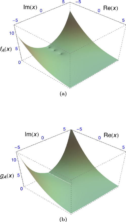
Figure 1: (Color online.) Figure (a) shows a contour plot of $f_{A}(x)=|{\mathrm{Ai}}(x)|^{1/6}$ as a function of $\mathrm{Re}(x)$ and $\mathrm{Im}(x)$. The exponent ${\textstyle{1\over 6}}$ is introduced in order to prevent “overflow” of the plotted function near the boundaries of the considered range of arguments. Figure (b) shows a contour plot of $|\exp(-{\textstyle{2\over 3}}\,x^{3/2})|^{1/6}$ as a function of $\mathrm{Re}(x)$ and $\mathrm{Im}(x)$. For $x<0$, i.e. on the negative real axis, the modulus is unity (Stokes line). The zeros of ${\mathrm{Ai}}(x)$ give rise to the visible “bump holes” on the negative real axis in panel (a). Except for the region near $\arg(x)=\pm\pi$, the Airy ${\mathrm{Ai}}$ function can be described using a single, uniform asymptotic formula $A(x)$ as defined in Eq. (24), which is proportional to $|\exp(-{\textstyle{2\over 3}}\,x^{3/2})|^{1/6}$.

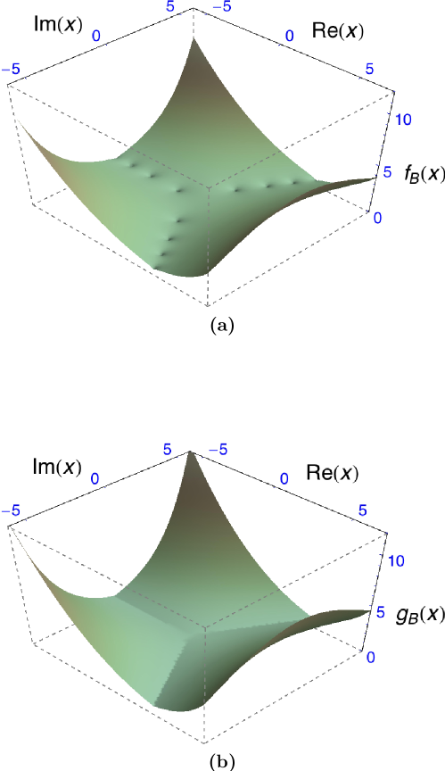
Figure 2: (Color online.) Figure (a) shows a plot of $|{\mathrm{Bi}}(x)|^{1/6}$ as a function of $\mathrm{Re}(x)$ and $\mathrm{Im}(x)$. From the contour plot, it is evident that a simple exponential of the form $|\exp(\pm{\textstyle{2\over 3}}\,x^{3/2})|^{1/6}$ cannot possibly describe the asymptotic behavior of the Airy ${\mathrm{Bi}}$ function. The zeros of ${\mathrm{Bi}}(x)$ give rise to visible “bump holes” on the negative real axis and along the lines $\arg(x)=\pm\pi/3$ in panel (a). Figure (b) shows a contour plot of $|f(x)|$ where $f(x)=|\exp({\textstyle{2\over 3}}\,x^{3/2})|^{1/6}$ for $|\arg(x)|\leq\pi/3$ and $f(x)=|\exp(-{\textstyle{2\over 3}}\,x^{3/2})|^{1/6}$ for $\pi/3<|\arg(x)|\leq\pi$, representing the Stokes line behavior near $\arg(x)=\pm\pi/3$ and $\arg(x)=\pi$ [see Eq. (27)].

III.2 Evaluation of the Airy function

We now discuss the principle of asymptotic overlap in the evaluation of the Airy functions of the first and second kind. In contrast to the usual notation, we denote the complex argument of the Airy functions as $x$, in order to distinguish it from the argument $z$ of the Bessel and Hankel functions. For $x\to 0$, we use the expansion,

$${\mathrm{Ai}}(x)= \;\sum_{k=0}^{\infty}\frac{3^{-2k-{\textstyle{2\over 3}}}}{k!\,\Gamma\left(k+{\textstyle{2\over 3}}\right)}\,x^{3\,k}-\sum_{k=0}^{\infty}\frac{3^{-2k-{\textstyle{4\over 3}}}}{k!\,\Gamma\left(k+{\textstyle{4\over 3}}\right)}\,x^{3\,k+1}\,.$$ (22a)

For the derivative of the Airy function, we have

$${\mathrm{Ai}}^{\prime}(x)= \;-\sum_{k=0}^{\infty}\frac{3^{-2k-{\textstyle{1\over 3}}}}{k!\,\Gamma(k+{\textstyle{1\over 3}})}\,x^{3\,k}+\sum_{k=0}^{\infty}\frac{3^{-2k-{\textstyle{5\over 3}}}}{k!\,\Gamma(k+{\textstyle{5\over 3}})}\,x^{3\,k+2}\,.$$ (22b)

The Airy $${\mathrm{Bi}}$$ function is given by

$${\mathrm{Bi}}(x)= \;\sum_{k=0}^{\infty}\frac{3^{-2k-{\textstyle{1\over 6}}}}{k!\,\Gamma(k+{\textstyle{2\over 3}})}\,x^{3\,k}+\sum_{k=0}^{\infty}\frac{3^{-2k-{\textstyle{5\over 6}}}}{k!\,\Gamma(k+{\textstyle{4\over 3}})}\,x^{3\,k+1}\,,$$ (22c)

and its derivative by

$${\mathrm{Bi}}^{\prime}(x)= \;\sum_{k=0}^{\infty}\frac{3^{-2k+{\textstyle{1\over 6}}}}{k!\,\Gamma(k+{\textstyle{1\over 3}})}\,x^{3\,k}+\sum_{k=0}^{\infty}\frac{3^{-2k-{\textstyle{7\over 6}}}}{k!\,\Gamma(k+{\textstyle{5\over 3}})}\,x^{3\,k+2}\,.$$ (22d)

The convergence radius of the expansions (22) is actually infinite, because of the Gamma functions in the denominator. Still, they are faced with numerical problems for large negative $x$. In order to illustrate this fact, we draw an analogy to the (likewise convergent) expansion $\exp(-x)=\sum_{k=0}^{\infty}(-1)^{k}x^{k}/k!$, which also involves a power in the numerator and a factorial in the denominator. Being absolutely convergent, this expansion is numerically useless for the evaluation of $\exp(-x)$ at $x=5000$, because the largest term in the series is of order $\exp(5000)$, whereas the entire sum amounts to $\exp(-5000)\approx 3.37\times 10^{-2172}$. If the series were summed term by term, one would incur a numerical loss of more than 4000 decimals. Other methods (asymptotic expansions for large argument) therefore have to be pursued. Figures 1 and 2 show the Stokes phenomenon. From Fig. 2, we infer that the Airy ${\mathrm{Bi}}$ integral is exponentially growing for $|x|\to\infty$, along the complex directions $\arg(x)=0$ and $\arg(x)=\pm 2\pi/3$, with Stokes lines at $\arg(x)=\pm\pi/3$ and $\arg(x)=\pi$. Therefore, the ${\mathrm{Bi}}$ integral cannot be represented by a simple asymptotic divergent series but must be the sum of two. This can be justified on the basis of saddle point considerations Ol1954asymp1 .

The expansions (22) are valid for $x\to 0$. Complementing these expansions, for $x\to\infty$, one is interested in suitable asymptotic expansions of the Airy functions. To this end, it is useful to relate the Airy ${\mathrm{Ai}}$ and ${\mathrm{Bi}}$ functions to a modified Bessel functions $K$ and $I$ of order $\pm{\textstyle{1\over 3}}$,

$${\mathrm{Ai}}(x)= \;\frac{1}{\pi}\,\sqrt{\frac{x}{3}}\,K_{{\textstyle{1\over 3}}}\!\!\left(\frac{2}{3}\,x^{3/2}\right),$$ (23a)

$${\mathrm{Bi}}(x)= \;\sqrt{\frac{x}{3}}\,\left[I_{{\textstyle{1\over 3}}}\left(\frac{2}{3}\,x^{3/2}\right)+I_{-{\textstyle{1\over 3}}}\left(\frac{2}{3}\,x^{3/2}\right)\right]\,.$$ (23b)

Based on the relationship of the Airy functions to modified Bessel functions, we infer that the following asymptotic series are relevant for the calculation of the Bessel functions at large argument,

$$A(x)= \;\frac{\exp\left(-{\textstyle{2\over 3}}\,x^{3/2}\right)}{\pi^{3/2}\,x^{1/4}}$$

$$\;\times\sum_{k=0}^{\infty}\frac{(-3)^{k}\,\Gamma\left(k+{\textstyle{1\over 6}}\right)\,\Gamma\left(k+{\textstyle{5\over 6}}\right)}{2^{2k+2}\,k!\;\;x^{3k/2}}\,,$$ (24a)

$$B(x)= \;\frac{\exp\left({\textstyle{2\over 3}}\,x^{3/2}\right)}{\pi^{3/2}\,x^{1/4}}$$

$$\;\times\sum_{k=0}^{\infty}\frac{3^{k}\,\Gamma\left(k+{\textstyle{1\over 6}}\right)\,\Gamma\left(k+{\textstyle{5\over 6}}\right)}{2^{2k+2}\,k!\;\;x^{3k/2}}\,,$$ (24b)

$$C(x)= \;\frac{x^{1/4}\,\exp\left(-{\textstyle{2\over 3}}\,x^{3/2}\right)}{\pi^{3/2}}\,$$

$$\;\times\sum_{k=0}^{\infty}\frac{(-3)^{k}\,\Gamma\left(k-{\textstyle{1\over 6}}\right)\,\Gamma\left(k+{\textstyle{7\over 6}}\right)}{2^{2k+2}\,k!\;\;x^{3k/2}}\,,$$ (24c)

whereas $$D(x)$$ is the only function that carries an overall minus sign in the prefactor,

$$D(x)= \;-\frac{x^{1/4}\,\exp\left({\textstyle{2\over 3}}\,x^{3/2}\right)}{\pi^{3/2}}\,$$

$$\;\times\sum_{k=0}^{\infty}\frac{3^{k}\,\Gamma\left(k-{\textstyle{1\over 6}}\right)\,\Gamma\left(k+{\textstyle{7\over 6}}\right)}{2^{2k+2}\,k!\;\;x^{3k/2}}\,.$$ (24d)

These series are generalized hypergeometric series of the ${}_{2}F_{0}$ form that diverge for every nonzero argument $x^{-3/2}$ unless they terminate. Their asymptotic relation to the Airy functions is clarified below. Indeed, the asymptotic expansions of ${\mathrm{Ai}}$ and ${\mathrm{Bi}}$ and of their derivatives can be related to the series $A(x)$, $B(x)$, $C(x)$ and $D(x)$. For $|x|\to\infty$, we have the divergent asymptotic expansion as a function of the complex phase,

$${\mathrm{Ai}}(x)\sim \;A(x)\,,$$

$$\;|x|\to\infty\,,\quad|\arg(x)|\leq\pi-\epsilon\,,$$ (25a)

$${\mathrm{Ai}}(x)\sim \;A(x)+{\mathrm{i}}\,B(x)\,,$$

$$\;|x|\to\infty\,,\quad\pi-\epsilon<\arg(x)\leq\pi\,,$$ (25b)

$${\mathrm{Ai}}(x)\sim \;A(x)-{\mathrm{i}}\,B(x)\,,$$

$$\;|x|\to\infty\,,\quad-\pi<\arg(x)<-\pi+\epsilon\,,$$ (25c)

For the derivative of the Ai function, we have

$${\mathrm{Ai}}^{\prime}(x)\sim \;C(x)\,,$$

$$\;|x|\to\infty\,,\quad|\arg(x)|\leq\pi-\epsilon\,,$$ (26a)

$${\mathrm{Ai}}^{\prime}(x)\sim \;C(x)+{\mathrm{i}}\,D(x)$$

$$\;|x|\to\infty\,,\quad\pi-\epsilon<\arg(x)\leq\pi\,,$$ (26b)

$${\mathrm{Ai}}^{\prime}(x)\sim \;C(x)-{\mathrm{i}}\,D(x)$$

$$\;|x|\to\infty\,,\quad-\pi<\arg(x)<-\pi+\epsilon\,,$$ (26c)

for arbitrarily small $\epsilon$. The role of the $\epsilon$ parameter in these expressions can be clarified as follows. From the formulas, it is evident that $\arg(x)\to\pm\pi$ (from below or above, respectively), there is an admixture of the asymptotic $B$ and $D$ series to the $A$ and $C$ series. The magnitude of that admixture is related to the magnitude of $|x|$. For large $|x|$, we can choose $\epsilon$ to be small. For finite $\epsilon$, one has to compare the magnitude of the two contributions. If the subdominant saddle point is numerically significant, one has to add its contributions (see also Fig. 3 below).

The dominant contributions to the asymptotic expansions for the Airy ${\mathrm{Bi}}$ functions are given by

$${\mathrm{Bi}}(x)\sim \;2\,B(x)\,,$$

$$\;|x|\to\infty\,,\quad|\arg(x)|<\frac{\pi}{3}-\epsilon\,,$$ (27a)

$${\mathrm{Bi}}(x)\sim \;2B(x)+{\mathrm{i}}\,A(x)\,,$$

$$\;|x|\to\infty\,,\quad\frac{\pi}{3}-\epsilon<\arg(x)<\frac{\pi}{3}+\epsilon\,,$$ (27b)

$${\mathrm{Bi}}(x)\sim \;{\mathrm{i}}\,A(x)\,,$$

$$\;|x|\to\infty\,,\quad\frac{\pi}{3}+\epsilon<\arg(x)<\pi-\epsilon\,,$$ (27c)

$${\mathrm{Bi}}(x)\sim \;B(x)+{\mathrm{i}}\,A(x)\,,$$

$$\;|x|\to\infty\,,\quad\pi-\epsilon<\arg(x)\leq\pi\,.$$ (27d)

For $$\arg(x)<0$$, the corresponding conditions are obtained by complex conjugation,

$${\mathrm{Bi}}(x)\sim \;2B(x)-{\mathrm{i}}\,A(x)\,,$$

$$\;|x|\to\infty\,,\quad-\frac{\pi}{3}-\epsilon<\arg(x)<-\frac{\pi}{3}+\epsilon\,,$$ (27e)

$${\mathrm{Bi}}(x)\sim \;-{\mathrm{i}}\,A(x)\,,$$

$$\;|x|\to\infty\,,\quad-\frac{\pi}{3}+\epsilon<\arg(x)<-\pi+\epsilon\,,$$

$${\mathrm{Bi}}(x)\sim \;B(x)-{\mathrm{i}}\,A(x)\,,$$

$$\;|x|\to\infty\,,\quad-\pi<\arg(x)\leq-\pi+\epsilon\,.$$ (27f)

The asymptotics for the derivative of the Airy ${\mathrm{Bi}}$ function are obtained by making the following replacements in Eq. (27): ${\mathrm{Bi}}\to{\mathrm{Bi}}^{\prime}$, $A\to C$, and $B\to D$.

The “principal of asymptotic overlap” which has been employed for a number of special functions in Ref. CaEtAl2007 would now call for an application of the power series (22a), (22b), (22c) and (22d) for small $|x|<R_{0}$, and for the use of the asymptotic expansions (25), (26) and (27) for $|x|>R_{1}$, with the region $R_{0}<|x|<R_{1}$ being bridged by the application of a nonlinear sequence transformation to the asymptotic expansions (25), (26), and (27). However, the situation is more complicated in reality, and it is impossible to choose the parameters $R_{0}$ and $R_{1}$ uniformly in the complex plane, independent of the complex phase of the argument $x$.

A possible scheme which is sufficient to obtain at least 20 digits of accuracy for all $x$ is outlined in Fig. 3. The designation “POWER” indicates the use of the power series (22a), (22b), (22c) and (22d), as appropriate, the designation “ASYMP” indicates the application of the asymptotic expansions (25), (26), and (27), where the series $A(x)$ and $B(x)$ are given in Eqs. (24) and (24). Finally, the designation “TRAFO” needs to be explained: it denotes the application of a nonlinear sequence transformation to the asymptotic series, with the aim of extending their validity to lower modulus of the argument than what they would otherwise be valid for.

A rather thorough discussion of an application of sequence transformation to a nontrivial problem has been given in Section 2.4.2 of Ref. CaEtAl2007 , in the context of the relativistic Green function for the hydrogen atom. Essentially, sequence transformations are generalizations of Padé approximations that fulfill accuracy-through-order relations, i.e., they constitute rational functions that reproduce the first few terms of a given input series when expanded back in powers of the argument. By reformulating the sequence transformation in terms of optimized remainder estimates We1989 , one can enhance the rate of convergence as compared to Padé approximations. A more thorough discussion of sequence transformation would go beyond the scope of the current article. The sequence transformation used in the current article is defined as follows. Let $s_{n}$ denote the $n$th partial sum of a series

$$s_{n}=\sum_{k=0}^{n}a_{k}\,,\qquad m=1,2,\dots,$$ (28)

where the $a_{n}$ are the terms in the series to be summed, and in our case, the terms in the asymptotic expansions (24). Let the difference operator $\Delta$ be explained as

$$\Delta s_{n}=s_{n+1}-s_{n}=a_{n+1}\,.$$ (29)

As described in Refs. We1989 ; CaEtAl2007 ; We2010 (see also §3.9 of Ref. OlLoBoCl2010 ), in many cases the following sequence transformation (Weniger transformation),

$${\delta}_{k}^{(n)}(\beta,s_{n})=\frac{\displaystyle\sum_{j=0}^{k}(-1)^{j}\left(\begin{array}[]{c}k\\ j\end{array}\right)\frac{(\beta+n+j)_{k-1}}{(\beta+n+k)_{k-1}}\frac{s_{n+j}}{\Delta s_{n+j}}}{\displaystyle\sum_{j=0}^{k}(-1)^{j}\left(\begin{array}[]{c}k\\ j\end{array}\right)\frac{(\beta+n+j)_{k-1}}{(\beta+n+k)_{k-1}}\frac{1}{\Delta s_{n+j}}}$$ (30)

leads to an accelerated convergence (or summation in the case of divergence) of the input sequence $\{s_{n}\}_{n=0}^{\infty}$ of partial sums of the series of the $a_{k}$. Here, $\beta$ is a shift parameter which we choose as $\beta=1$ (as given in Refs. We1989 ; CaEtAl2007 ). The starting order for the transformation in Eq. (30) is $n$ which we choose to be $n=0$. Then, ${\delta}_{k}^{(0)}(\beta,s_{0})$ denotes the $k$th order Weniger transform of the input sequence $\{s_{n}\}_{n=0}^{\infty}$. The central idea in the construction of the sequence transformation (30) is the expansion of the remainder term in an inverse factorial series, as explained in Ref. We1989 . The use of recursion relations described in Section 8.3 of Ref. We1989 is imperative in order to ensure the computational efficiency and numerical stability in the computations of the Weniger transforms. In Refs. We1989 ; We1996c ; CaEtAl2007 , it has been established that the Weniger transformation is very powerful at summing the factorially divergent series that result from the asymptotic expansions of special functions in terms of hypergeometric series.

We find, by comparison to calculations with extended arithmetic using computer algebra systems Wo1988 and by comparison of different methods along the separating domains indicated in Fig. 3, that naive termination criteria are sufficient in order to reach a prescribed accuracy of 20 decimals in the entire complex plane, for the Airy functions. By a naive termination criterion, we mean that the summation of terms in the power series, or the summation of terms in the asymptotic series, is terminated when the next higher-order term divided by the most recently calculated partial sum is a factor 100 less than the prescribed accuracy for the evaluation of the Airy function. Likewise, the calculation of subsequent higher-order transforms ${\delta}_{k}^{(0)}$ of the Weniger transform (30) is terminated when the apparent convergence of three consecutive transform (maximum absolute value of the relative difference of transforms $k$, $k+1$ and $k+2$) is smaller than the prescribed accuracy by a factor of 100.

The appropriate evaluation method for given complex argument $x$ is indicated in Fig. 3, as a function of $\mathrm{Re}(x)$ and $\mathrm{Im}(x)$. The derivatives ${\mathrm{Ai}}^{\prime}(x)$ and ${\mathrm{Bi}}^{\prime}(x)$ are evaluated using the same schemes as ${\mathrm{Ai}}(x)$ and ${\mathrm{Bi}}(x)$, respectively, but (for the asymptotic regime of large argument) with the replacements $A\to C$, and $B\to D$ [see Eq. (24)]. We should also clarify the exact formulas for some of the separating curves in Figs. 3(a) and 3(b). The curved separating line between “TRAFO” and “POWER” in Fig. 3(a) follows the formula

$$|x|<5+\frac{15}{\pi}\,|\arg(x)|\,,\quad|\arg(x)|<\frac{2\pi}{3}\,,$$ (31)

and it meets the outer asymptotic region “ASYMP” at $|\arg(x)|=\frac{2\pi}{3}$ and $|x|=15$. In Fig. 3(a), the transition from the asymptotic series $A$ to the asymptotic series $A+{\mathrm{i}}\,B$ takes place at $\arg(x)=\pm\frac{5\pi}{6}$. In Fig. 3(b), for the ${\mathrm{Bi}}$ integral, the power series is used for $|x|<5$ uniformly for any complex phase of $x$. For $|x|<15$, the power series is also used, but only for $|\arg(x)|<\pi/3$. The transition from the asymptotic series $2\,B$ to the asymptotic series $2\,B+{\mathrm{i}}A$ takes place for $|x|\geq 15$, and $\arg(x)=\pm\pi/6$.

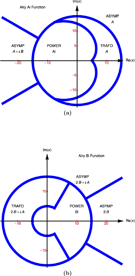
Figure 3: (Color online.) Algorithms used for the Airy ${\mathrm{Ai}}$ function [panel (a)] and for the Airy ${\mathrm{Bi}}$ function [panel(b)]. The explanation is in the text.

III.3 Summation of uniform asymptotics

The uniform asymptotic formulas (III.1), (III.1), (III.1) and (III.1) are expansions for large $\nu$ for argument $z=\nu\,y$ of the Bessel functions. They can be written in a form that is amenable to the application of the convergence acceleration transformation (30), as follows. We consider as an example Eq. (III.1). Then,

$$J_{\nu}(\nu\,y)\sim \;\sum_{k=0}^{\infty}\tilde{a}_{k}\,,\qquad\tilde{s}_{n}=\sum_{k=0}^{n}\tilde{a}_{k}\,,$$ (32a)

$$\tilde{a}_{k}= \;\left(\frac{4\zeta}{1-y^{2}}\right)^{1/4}\,\left\{\frac{{\mathrm{Ai}}(\nu^{2/3}\,\zeta)}{\nu^{1/3}}\;\frac{a_{k}(\zeta)}{\nu^{2k}}\right.$$

$$\left.+\frac{{\mathrm{Ai}}^{\prime}(\nu^{2/3}\,\zeta)}{\nu^{5/3}}\;\frac{b_{k}(\zeta)}{\nu^{2k}}\right\}\,.$$ (32b)

Here, the Airy functions need to be evaluated only once as they do not depend on $k$. Treating the Airy function term and the derivative term together (i.e., as a single term $\tilde{a}_{k}$), we empirically observe better convergence in many cases. Written in the form (32), the convergence of the uniform asymptotic for the Bessel $J$ function can be accelerated by calculating the transforms ${\delta}_{k}^{(n)}(\beta,\tilde{s}_{n})$ where again, we choose $n=0$ in the current investigation. We empirically observe that the use of the convergence accelerator does not induce any stability issue even in cases ($\nu\neq z$) where the apparent convergence of the asymptotic series would be sufficient to calculate the Bessel $J$ function to the required accuracy.

A special case still necessitates a modification of the algorithm. Namely, for large and almost equal $\nu$ and $z$, the confluence of the two saddle points defining the Bessel function (see Appendix A below) leads to numerically prohibitive cancellations in evaluating the series of the $a_{k}(\zeta)$ and $b_{k}(\zeta)$ coefficients. It is impossible to overcome these difficulties with the necessarily finite precision of computer systems in the limit $z\to\nu$; indeed, as described below in Section IV, the asymptotic expansions for large $\nu$ at exact equality $\nu=z$ are obtained after the cancellation of a number of divergent terms in $\epsilon$ after setting $\nu=z+\epsilon$.

Eventually, we find that the region in very close vicinity of the turning point $\nu=z$ can only be overcome by an explicit use of the recurrence relation

$${\cal J}_{\nu-1}(x)+{\cal J}_{\nu+1}(x)=\frac{2\nu}{x}\,{\cal J}_{\nu}(x)\,,$$ (33)

with the notion of displacing $\nu$ from $z$, where again ${\cal J}$ stands for $J$, $Y$, $H^{(1)}$ or $H^{(2)}$. We find that numerical cancellations are most severe when $\nu$ is slightly lower than $\mathrm{Re}(z)$. So, for $\mathrm{Re}(z)-21<\nu<\mathrm{Re}(z)+2$, we therefore express ${\cal J}_{\nu}(z)$ as a function of ${\cal J}_{\nu+24}(z)$ and ${\cal J}_{\nu+25}(z)$ by repeated use of the recurrence relation (33). Indeed, by repeated application of Eq. (33) one can express ${\cal J}_{\nu}(z)$ as

$${\cal J}_{\nu}(z)=f_{24}(\nu,z)\;{\cal J}_{\nu+24}(z)+f_{25}(\nu,z)\;{\cal J}_{\nu+25}(z)\,,$$ (34)

where $f_{24}$ and $f_{25}$ are somewhat lengthy rational functions of their arguments. Their explicit form can easily be obtained using computer algebra Wo1988 .

The recurrence relation (34) is applied in the direction of increasing order $\nu$ of the Bessel function, where it may be be unstable [indeed, $J_{\nu}(z)\to 0$ and $Y_{\nu}(z)\to\infty$ for $\nu\to\infty$ at constant $z$]. One might thus expect that the shift (34) could induce numerical instability. However, because the shift is applied in the region $\nu\approx z$, where the Bessel function is not yet in its asymptotic regime for large $\nu\gg z$, the numerical cancellations are only minor and do not constitute a matter of concern.

III.4 Numerical examples

In order to demonstrate the power of the algorithms proposed in the current article, we now turn our attention to a number of numerical example cases. We first present two evaluations for non-integer order and argument of Bessel functions, in the range $\nu\approx z$, which result in

$$J_{5\,000\,000.2}(5\,000\,000.1)=2.614\,463\,954\,691\,926\times 10^{-3}\,,$$ (35)

and in

$$Y_{5\,000\,000.2}(5\,000\,000.1)=-4.533\,251\,771\,400\,041\times 10^{-3}\,.$$ (36)

For an example with $\arg(z)=\pi/3$, we obtain

$$H^{(1)}_{5\,000\,000.2}(5\,000\,000.1\,\exp({\mathrm{i}}\pi/3))$$

$$\qquad=-6.120\,398\,939\,598\,734\times 10^{-954990}$$

$$\qquad\qquad-{\mathrm{i}}\,1.992\,559\,471\,616\,042\times 10^{-954989}\,.$$ (37)

While the result is nearly zero, numerical evaluations of this kind are needed because other terms in angular momentum expansions in quantum electrodynamics lead to extremely slowly convergent series JeMoSo1999 ; JeMoSo2001pra due to an interplay of increasing and decreasing terms (as the angular momentum quantum number is increased). Another example of explicit evaluation of the Hankel function for extremely large order and argument in the turning point regime $\nu\approx z$ reads,

$$H^{(1)}_{6\,000\,000.2}(6\,000\,000.7)$$ (38)

$$\qquad=2.467\,848\,322\,382\,092\times 10^{-3}$$

$$\qquad\qquad-{\mathrm{i}}\,4.252\,887\,224\,934\,845\times 10^{-3}\,,$$

and

$$H^{(2)}_{6\,000\,000.2}(6\,000\,000.7)=$$ (39)

$$\qquad 2.467\,848\,322\,382\,092\times 10^{-3}$$

$$\qquad\qquad+{\mathrm{i}}\,4.252\,887\,224\,934\,845\times 10^{-3}\,.$$

For $r\approx 1$, it is instructive to verify the Bessel functions using the following sum rule,

$$\frac{\exp\bigl{(}-y[1-r]\bigr{)}}{y[1-r]}\;=\;-\,\sum_{\ell=0}^{\infty}(2l+1)\,j_{\ell}({\mathrm{i}}\,r\,y)\,h^{(1)}_{\ell}({\mathrm{i}}\,y)\,,$$ (40)

for $r\in(0,1)$ and $y>0$. The sum over $\ell$ constitutes a slowly convergent series whose can otherwise by accelerated using the combined nonlinear-condensation transformation JeMoSoWe1999 . The sum rule directly follows from the angular momentum expansion of the Green function of the Helmholtz equation for the case of collinear arguments, as given in Chap. 9 of Ref. Ja1998 . It can also be derived as a reformulation of Eq. (10.60.3) of Ref. OlLoBoCl2010 . We have checked our values of the Bessel functions on the basis of this sum rule and plotted Bessel functions of high order in the turning point region (see Figs. 4 and 5).

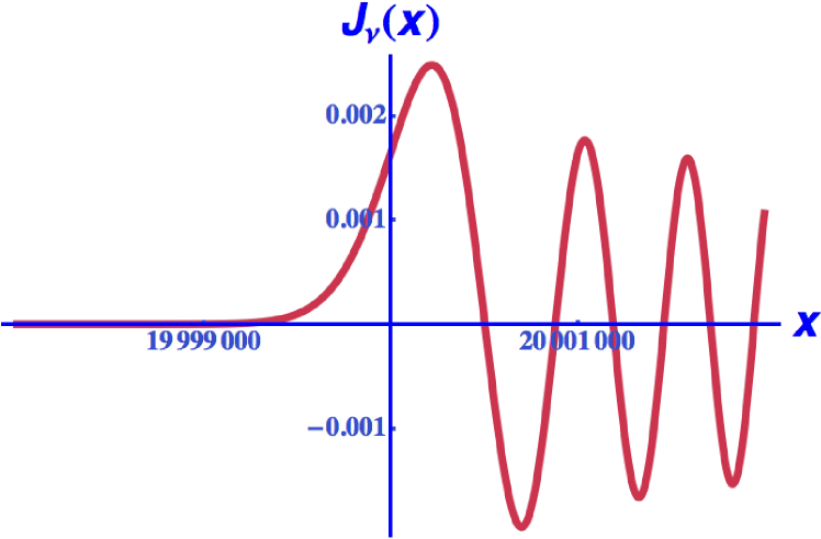
Figure 4: Plot of the Bessel function $J_{\nu}(x)$ with $\nu=20,000,000.2$ in the turning point region.

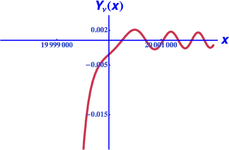
Figure 5: Plot of the Bessel function $Y_{\nu}(x)$ with $\nu=20,000,000.2$ in the turning point region.

IV ASYMPTOTICS AT THE TURNING POINT

The direct application of the uniform asymptotics becomes problematic when the argument and the order of a Bessel function are almost equal, because of numerical cancellations involved in evaluating the individual coefficients in this case. We remember that for the case $\nu\approx z$, special methods have to be employed for the summation of the uniform asymptotic expansion (see Section III.3). This is because of highly significant numerical cancellations in the evaluation of the sums defining $a_{k}$ and $b_{k}$ given in Eqs. (15a) and (15b). These numerical cancellations reflect the confluence of the two saddle discussed below in Appendix A and are present even if the sums in Eqs. (15a) and (15b) are finite.

Nevertheless it is possible to investigate the limit $\nu\to z$ by an analytic expansion setting $\nu=z+\epsilon$. In the calculation, the result is obtained only after the cancellation of a few divergent terms which are inverse powers of $\epsilon$. For exact equality $\nu=z$, it is possible to derive analytic approximations. These serve as an important test device for the numerical algorithms. The results given in formulas (9.3.31)–(9.3.34) of Ref. AbSt1972 for lower order terms in the asymptotic expansions do not reach a sufficiently high order in order to be useful for the current investigation, and we have thus calculated a few more terms in the asymptotic expansions of $J_{\nu}(\nu)$ and $Y_{\nu}(\nu)$ for $\nu\to\infty$.

The general structure of the asymptotic expansions is as follows,

$$J_{\nu}(\nu)= \;\frac{a}{\nu^{1/3}}\,\sum_{k=0}^{\infty}\frac{\alpha_{k}}{\nu^{2\,k}}-\frac{b}{\nu^{5/3}}\,\sum_{k=0}^{\infty}\frac{\beta_{k}}{\nu^{2\,k}}\,,$$ (41a)

$$Y_{\nu}(\nu)= \;-\frac{3^{1/2}\,a}{\nu^{1/3}}\,\sum_{k=0}^{\infty}\frac{\alpha_{k}}{\nu^{2\,k}}-\frac{3^{1/2}\,b}{\nu^{5/3}}\,\sum_{k=0}^{\infty}\frac{\beta_{k}}{\nu^{2\,k}}\,,$$ (41b)

$$J^{\prime}_{\nu}(\nu)= \;\frac{b}{\nu^{2/3}}\,\sum_{k=0}^{\infty}\frac{\gamma_{k}}{\nu^{2\,k}}-\frac{a}{\nu^{4/3}}\,\sum_{k=0}^{\infty}\frac{\delta_{k}}{\nu^{2\,k}}\,,$$ (41c)

$$Y^{\prime}_{\nu}(\nu)= \;=\frac{3^{1/2}\,b}{\nu^{2/3}}\,\sum_{k=0}^{\infty}\frac{\gamma_{k}}{\nu^{2\,k}}+\frac{3^{1/2}\,a}{\nu^{4/3}}\,\sum_{k=0}^{\infty}\frac{\delta_{k}}{\nu^{2\,k}}\,.$$ (41d)

The constants $a$ and $b$ are given by AbSt1972

$$a=\frac{2^{1/3}}{3^{2/3}\,\Gamma(2/3)}\,,$$ (42)

and

$$b=-\frac{2^{2/3}}{3^{1/3}\,\Gamma(1/3)}\,.$$ (43)

Numerical values of the coefficients $\alpha_{k}$, $\beta_{k}$, $\gamma_{k}$, $\delta_{k}$ were given in (unnumbered) equations following Eq. (9.3.34) of Ref. AbSt1972 , but only in numerical form. Using the formalism outlined in Refs. AbSt1972 ; Wa1922 ; Ma1993bessel , and computer algebra Wo1988 , it is relatively easy to evaluate these coefficients analytically. The first terms read

$$\alpha_{0}= \;1\,,\qquad\alpha_{1}=-\frac{1}{225}\,,\qquad\alpha_{2}=\frac{151439}{218295000}\,,$$

$$\alpha_{3}= \;-\frac{887278009}{2504935125000}\,,$$

$$\alpha_{4}= \;\frac{1374085664813273149}{3633280647121125000000}\,,$$

$$\alpha_{5}= \;-\frac{1065024810026227256263721}{1540965154460247140625000000}\,.$$ (44)

for the $\alpha_{k}$ coefficients. For $\alpha_{j}$ with $j=6,7,8$, the integers in the numerator and denominator are too long to be displayed, practically. The results read, up to 30 decimals,

$$\alpha_{6}= \;0.00192\,82196\,42487\,75701\,38042\,30112\,,$$

$$\alpha_{7}= \;-0.00762\,60912\,66562\,73551\,11507\,07644\,,$$

$$\alpha_{8}= \;0.04059\,16252\,02439\,02610\,46110\,96353\,.$$ (45)

We obtain for the $\beta_{k}$,

$$\beta_{0}= \;\frac{1}{70}\,,\qquad\beta_{1}=-\frac{1213}{1023750}\,,$$

$$\beta_{2}= \;\frac{16542537833}{37743205500000}\,,\beta_{3}=-\frac{9597171184603}{25476663712500000}\,,$$

$$\beta_{4}= \;\frac{53299328587804322691259}{91182706744837207500000000}\,,$$

$$\beta_{5}= \;-\frac{70563256104582737796094772987}{49341242187300033908437500000000}\,.$$ (46)

For $\beta_{j}$ with $j=6,7,8$, the results read, up to 30 decimals,

$$\beta_{6}= \;0.00506\,84595\,77410\,25775\,49192\,90289\,,$$

$$\beta_{7}= \;-0.02455\,31387\,44039\,61140\,77960\,53629\,,$$

$$\beta_{8}= \;0.15584\,22313\,83604\,27406\,01873\,20654\,.$$ (47)

The results for the $\gamma_{k}$ read,

$$\gamma_{0}= \;1\,,\qquad\gamma_{1}=\frac{23}{3150}\,,\qquad\gamma_{2}=-\frac{604523}{644962500}\,,$$

$$\gamma_{3}= \;\frac{2264850139339}{5095332742500000}\,,$$

$$\gamma_{4}= \;-\frac{160913976870912403}{353106559055250000000}\,,$$

$$\gamma_{5}= \;\frac{216363828773939104866579281}{266709417228648831937500000000}\,.$$ (48)

For $\gamma_{6}$, $\gamma_{7}$, and $\gamma_{8}$, we again give numerical results, up to 30 decimals,

$$\gamma_{6}= \;-0.00222\,15829\,52781\,90513\,99808\,25549\,,$$

$$\gamma_{7}= \;0.00866\,43390\,74500\,57903\,06978\,05128\,,$$ (49)

$$\gamma_{8}= \;-0.04561\,48821\,43058\,95740\,37593\,20268\,.$$

Finally, we obtain for the $\delta_{k}$,

$$\delta_{0}= \;\frac{1}{5}\,,\qquad\delta_{1}=-\frac{947}{346500}\,,$$ (50)

$$\delta_{2}= \;\frac{11192989}{18555075000}\,,\delta_{3}=-\frac{100443412440047}{262141460831250000}\,,$$

$$\delta_{4}= \;\frac{11007971229145235539}{22905464949241875000000}\,,$$

$$\delta_{5}= \;-\frac{180026595127347603856424798473}{180354561678027325338750000000000}\,.$$

The first 30 decimals of the results for $\delta_{6,7,8}$ read

$$\delta_{6}= \;0.00309\,74954\,54537\,99792\,65245\,46715\,,$$

$$\delta_{7}= \;-0.01341\,95416\,64085\,43255\,61825\,95640\,,$$

$$\delta_{8}= \;0.07735\,88016\,72766\,55151\,01508\,73624\,.$$ (51)

We have used these analytic formulas in our verification of numerical results obtained using the method described in Section III.

V CONCLUSIONS

We have described an algorithm for the evaluation of an individual Bessel or Hankel function for large order $\nu$, and arbitrary complex argument $z$. The method relies on the use of the uniform asymptotic expansions given in Eqs. (III.1), (III.1), (III.1) and (III.1). These asymptotic expansions involve ${\mathrm{Ai}}$ and ${\mathrm{Bi}}$ functions, and their derivatives. Consequently, in passing and also as a prerequisite for our algorithm, we need to develop numerical code for the Airy functions valid in the entire complex plane. This is described in Section III.2, and the appropriate algorithms for the different regions in the complex plane are given in Fig. 3. Essentially, these represent an adapted implementation of the “principle of asymptotic overlap” where a power series is used for small argument, an asymptotic expansion is used for large argument, and the region in between is bridged by a nonlinear sequence transformation [Weniger transformation, see Eq. (30)].

As evident from Fig. 3, this principle needs to be adapted for the Airy functions, and the regions separating the algorithms depend on the complex phase of the argument. Using the Airy function algorithm and the uniform asymptotic expansion, we obtain expressions for the Bessel and Hankel functions which can readily be evaluated for almost arbitrary values of $\nu$ and $z$. However, formidable numerical cancellations still prevent us from using the uniform asymptotic expansions directly when $\nu\approx z$. In this case, the region near $\nu=z$ is bridged by the application of a convergence accelerator (Weniger transformation), applied in this case to the infinite asymptotic series defining the expansion for large $\nu$ in the uniform asymptotic formulas (III.1), (III.1), (III.1) and (III.1). The transformation is applied after the order $\nu$ is shifted away [see Eq. (34)] by a finite amount from the argument $z$ using the recurrence formula satisfied by the Bessel function (10). Numerical examples are given in Section III.4.

In a typical application within physics, one needs Bessel functions for both real as well as complex argument. For example, in bound-state quantum electrodynamics (QED), one needs to describe complex photon energies. Therefore, it is highly desirable to have an algorithm that is applicable in the entire complex plane, for a Bessel function of large order. Here, we use a combination of ideas to overcome the severe difficulties faced by this endeavor. We use a nonlinear sequence transformation for the summation of asymptotic expansions for the Airy functions in order be able to use this expansion for small and moderate argument where the usual paradigm of truncating the asymptotics at the smallest term would otherwise yield dissatisfactory accuracy. The Stokes phenomenon must still be taken into account in terms of the complex phase of the argument of the Airy function. Finally, we overcome the remaining numerical difficulties in the summation of the uniform asymptotic expansion, associated with the turning point $\nu=z$, by a simple shift of the order versus the argument, and by the further use of the Weniger transformation for the summation of the uniform asymptotic expansion in the transition region near $\nu=z$.

Examples where Bessel functions of large argument and order are needed, include scattering problems and calculations with photon propagators and fermion propagators in atomic physics and field theory, and diverse technical application areas. Although it is possible to recursively evaluate arrays of Bessel functions of the same argument with varying order, the individual evaluation of Bessel functions in “extreme” argument ranges remains an elusive problem. Here, we attempt to address this problem via a combination of summation algorithms, convergence accelerators, recurrence relations and the “principle of asymptotic overlap,” adapted to the problem at hand. In passing, we also address the numerically accurate calculation of Airy functions in the entire complex plane. We leave it to the interested reader to develop their own implementation of the methods described here, adapted to the arithmetic accuracy requirements for the particular application in question.

Finally, let us indicate a few open problems in the area. We have outlined the general algorithm used in our evaluation of Bessel functions. The description of an implementation, including an example code, possibly with more refined termination criteria than those indicated in Section III.2 for the Airy functions, would certainly be of value to the scientific community. Secondly, in view of the considerations outlined below in Appendix A, it seems feasible to construct an equally powerful algorithm based on an adaptation of the saddle point integration. In this case, considerable care needs to be vested into the turning point case $\nu\approx z$ as well. Finally, preliminary investigations (not described here in any further detail) indicate that the Debye expansion, which is different from the uniform asymptotic expansion, may be used to good effect for the case of real $\nu$, and real argument $z$, of the Bessel function. The Debye expansion is given in Eqs. (9.3.7),. (9.3.8), (9.3.11) and (9.3.12) of Ref. AbSt1972 . The Debye expansion may be combined with convergence accelerators. It would be instructive and worthwhile to construct a complementary algorithm for Bessel and Hankel functions valid only for real argument.

Appendix A SADDLE POINT INTEGRATIONS

A.1 Orientation

In this Appendix, we explore alternative numerical procedures, with a special emphasis on numerical integration around saddle points. Before we come to a discussion of the procedure involved, let us briefly review other, alternative approaches to the calculation of Bessel and Hankel functions which have been discussed in the literature. In Ref. Te1994 , it has been advocated to directly integrate the defining differential equation in suitable directions in the complex plane. In Ref. ScAnGo1979 , an analogous approach has been advocated for the calculation of Airy functions. There is a further obvious problem at the turning point, where the argument $z$ and order $\nu$ of the Bessel function are nearly equal. In this case, there are huge numerical cancellations in the calculation of the expansion coefficients that multiply the Airy functions which are required in order to evaluate the uniform asymptotic expansions. In Ref. Te1997uniform , it has been suggested to avoid using the expansion in inverse powers of the order of the Bessel function in this case, and to use a convergent expansions in terms of a scaled complex argument $\zeta$ of the special function. The procedure advocated in Ref. Te1997uniform is applicable to the transition region $\nu\approx z$ where $\zeta\approx 0$, but cannot be universally applied when $\zeta$ is manifestly different from zero. Another method HoOD1999 is to expand the coefficients of the asymptotic expansion into hyperasymptotics. Yet, the asymptotic expansions of the coefficients of the asymptotic expansions (sic!) are not applicable to all cases of interest and introduce another level of complexity into the problem. Hadamard series expansions as an alternative to the uniform asymptotics (still equal in limiting cases) have been investigated in Refs. Pa2001hadamard1 ; Pa2001hadamard2 ; Pa2004hadamard3 . Finally, let us also mention that some special parameter cases of interest have received attention in the literature. For example, asymptotic expansions for Bessel functions of the third kind of imaginary order have been discussed in Refs. Ba1966 ; ShWo2009 .

However, the preeminent issue in the formulation of possible alternative evaluation methods for Bessel and Hankel functions seems to be connected with a numerical integration about saddle points in the complex plane. Expansions about the saddle points give rise to the above mentioned uniform asymptotic expansions (III.1), (III.1), (III.1) and (III.1). In general, the evaluation of Hankel, and Bessel functions can be written in terms of two saddle points which dominate the paths of integration. Expanding to second order about the saddle point, we obtain linear contours that approximate the paths of steepest descent and may be used in order to evaluate the functions, approximately. This approach, which has been advocated previously in Ma1993bessel and recently in SmdHTi2009 , is appealing because of its relative simplicity. Since the integrand of the integral defining $J_{\nu}(z)$ is in general highly oscillating, the integration paths must be chosen with care. Here, we describe a somewhat simplified approach, in which one approximates the ideal path by a short linear segment crossing the saddle point. Our treatment is similar to that in SmdHTi2009 , however, we pay special attention to the case when argument and order of the Bessel function are almost equal, which was not considered in SmdHTi2009 .

In the case of equal argument and order, $\nu=z$, the phenomenon of confluence of the two saddle points needs to be analyzed. For $\nu\approx z$, the two saddle points approach each other. For precise equality $\nu=z$, the two saddle points coalesce, and there are three paths of steepest descent, complemented by three paths of steepest ascent, about the saddle point. This leads to a more complicated situation with kinks in the contours of steepest descent, which must be used in order to evaluate the special functions. The investigations reported below are therefore of more general interest with respect to the numerical problems related to the confluence of the saddle points.

A.2 Complex integral representations

The defining integrals for the Hankel functions $H^{(1)}_{\nu}(z)$ and $H^{(2)}_{\nu}(z)$ read ($\operatorname{\textrm{Re}}z>0$, and arbitrary complex $\nu$)

$$H^{(1)}_{\nu}(z)= \;\frac{1}{\pi{\mathrm{i}}}\,\int_{-\infty-{\mathrm{i}}\pi}^{\infty}\exp\left(g(t)\right){\mathrm{d}}t,$$ (52a)

$$H^{(2)}_{\nu}(z)= \;\frac{1}{\pi{\mathrm{i}}}\int^{-\infty+{\mathrm{i}}\pi}_{\infty}\exp\left(g(t)\right){\mathrm{d}}t,$$ (52b)

with

$$g(t)=-z\sinh(t)+\nu t=-\nu\,(y\sinh(t)-t)\,.$$ (53)

Here we have introduced the variable $y=z/\nu$, which will prove convenient in the ensuing discussion. Combining the two Hankel functions to the Bessel function $J_{\nu}(z)=[H^{(1)}_{\nu}(z)+H^{(2)}_{\nu}(z)]/2$, we obtain from Eq. (52a) the integral representation for $J_{\nu}(z)$:

$$J_{\nu}(z)=\frac{1}{2\pi{\mathrm{i}}}\int^{-\infty+{\mathrm{i}}\pi}_{-\infty-{\mathrm{i}}\pi}\exp\left(g(t)\right)\,{\mathrm{d}}t.$$ (54)

The contour of integration (54) is arbitrary. It can be deformed, nevertheless, to pass through the saddle point. Finally, the Bessel function of the second kind is obtained as $Y_{\nu}(z)=[H^{(1)}_{\nu}(z)-H^{(2)}_{\nu}(z)]/(2{\mathrm{i}})=-{\mathrm{i}}\,[H^{(1)}_{\nu}(z)-J_{\nu}(z)]$.

The definition (52a) is valid provided $\operatorname{\textrm{Re}}z>0$, to ensure convergence of the integrals. The identity $\sinh(t-{\mathrm{i}}\pi)=\sinh(t+{\mathrm{i}}\pi)=-\sinh(t)$ is instrumental in deriving this condition. For $\operatorname{\textrm{Re}}(z)<0$, we apply the conversion formulas (6). The case of purely imaginary $z=x+{\mathrm{i}}\,y$ requires another integral representation. We may use

$$J_{\nu}({\mathrm{i}}|y|)= \;\exp\left(\frac{1}{2}\nu\pi{\mathrm{i}}\right)\,I_{\nu}(|y|),$$ (55)

$$J_{\nu}(-{\mathrm{i}}|y|)= \;\exp\left(-\frac{3}{2}\nu\pi{\mathrm{i}}\right)\,I_{\nu}(-|y|),$$ (56)

$$H_{\nu}^{(1)}({\mathrm{i}}|y|)= \frac{2}{\pi{\mathrm{i}}}{\mathrm{e}}^{-\frac{1}{2}\nu\pi{\mathrm{i}}}K_{\nu}(|y|),$$ (57)

$$H_{\nu}^{(2)}(-{\mathrm{i}}|y|)= -\frac{2}{\pi{\mathrm{i}}}{\mathrm{e}}^{\frac{1}{2}\nu\pi{\mathrm{i}}}K_{\nu}(|y|),$$ (58)

which expresses the Bessel functions in terms of modified Bessel functions $I_{\nu}(x)$ and $K_{\nu}(x)$. For $\operatorname{\textrm{Re}}(x)>0$, these have integral representations

$$I_{\nu}(x)= \;\frac{1}{\pi}\int_{0}^{\pi}\exp\left(x\cos\theta\right)\,\cos(\nu\theta){\mathrm{d}}\theta$$

$$\;-\frac{\sin(\nu\pi)}{\pi}\,\int_{0}^{\infty}\exp\left(-x\cosh t-\nu t\right)\,{\mathrm{d}}t,$$ (59a)

$$K_{\nu}(x)= \int_{0}^{\infty}\exp\left(-x\cosh t\right)\,\cosh(\nu t){\mathrm{d}}t\,.$$ (59b)

Negative arguments can be transformed to positive arguments via the relations

$$I_{\nu}(-x)= \;\exp\left(\nu\pi{\mathrm{i}}\right)\,I_{\nu}(x),$$ (60a)

$$K_{\nu}(-x)= \;\exp\left(-\nu\pi{\mathrm{i}}\right)\,K_{\nu}(x)-\pi{\mathrm{i}}I_{\nu}(x).$$ (60b)

A.3 Paths of steepest descent

We recall the definition of the integrand in the integral representation of the Bessel function,

$$g(t)=-\nu\,(y\,\sinh(t)-t)\,.$$ (61)

Expanded to second order about the saddle point $t=t_{j}$, to be specified below, one obtains

$$g(t)= \;g(t_{j})+g^{\prime}(t_{j})\,(t-t_{j})+\frac{1}{2}g^{\prime\prime}(t_{j})\,(t-t_{j})^{2}+\ldots$$

$$= \;-\nu\,\left(y\sinh(t_{j})-t_{j}\right)+\nu\left(1-y\cosh(t_{j})\right)\,(t-t_{j})$$

$$\;-\frac{1}{2}\,\nu\,y\,\sinh(t_{j})\,(t-t_{j})^{2}$$

$$\;-\frac{1}{6}\,\nu\,y\,\cosh(t_{j})\,(t-t_{j})^{3}+\dots\,.$$ (62)

The method of numerical evaluation of the functions $J_{\nu}(z)$ and $Y_{\nu}(z)$ amounts to finding approximations to the integrals (52a), (52b) by quadrature. The starting point is to find the saddle points $t_{\pm}$ of the integrand in (54). They satisfy $g^{\prime}(t_{\pm})=0=y\cosh t_{\pm}-1$, and are given as

$$t_{+}= \;\ln\left(\frac{1+\sqrt{1-y^{2}}}{y}\right)=a_{+}+{\mathrm{i}}\;b_{+},$$ (63a)

$$t_{-}= \;\ln\left(\frac{1-\sqrt{1-y^{2}}}{y}\right)=a_{-}+{\mathrm{i}}\;b_{-}=-t_{+}\,,$$ (63b)

for $|\operatorname{\textrm{Im}}t_{\pm}|\leq\pi$, and the notation $t_{\pm}=a_{\pm}+{\mathrm{i}}\,b_{\pm}$ (real $a_{\pm}$, $b_{\pm}$) is introduced for later use. Multiplying the arguments of the logarithms in Eq. (63), we see that the saddle points fulfill the relation $t_{+}+t_{-}=0$. Furthermore, we have $\operatorname{\textrm{Re}}t_{-}\leq 0$ (and $\operatorname{\textrm{Re}}t_{+}\geq 0$). For the case of equal argument and order, the two saddle point coalesce at the origin,

$$\nu=z\,,\qquad t_{+}=t_{-}=0\,.\qquad$$ (64)

The path of steepest descent (PSD) is a path $t$ in the complex plane, passing through the saddle point, such that the imaginary part of the exponent $g(t)$ is constant along this path. This means that the integrand $\exp\left(g(t)\right)$ does not oscillate. Of course, there are further saddle points in the complex plane, described by the formula $t_{\pm}+2n\pi{\mathrm{i}}$, $n$ integer, but these are not needed in our investigation.

In addition, the amplitude of the integrand $\exp\left(g(t)\right)$ decreases monotonically as we go along the path away from the saddle point. Together, these properties make numerical quadrature along the PSD easy. In order find an expression for the PSD, we write

$$t=\xi+{\mathrm{i}}\,\eta\,,$$ (65)

and require that the imaginary part of $g(t)$ remains constant along the path of integration. We write $z=z_{\textrm{R}}+{\mathrm{i}}\,z_{\textrm{I}}$, with $z_{\textrm{R}}=\operatorname{\textrm{Re}}z$ and $z_{\textrm{I}}=\operatorname{\textrm{Im}}z$, and in complete analogy, $\nu=\nu_{\textrm{R}}+{\mathrm{i}}\,\nu_{\textrm{I}}$. Then,

$$\operatorname{\textrm{Im}}g(t_{\pm})=\operatorname{\textrm{Im}}g(t)$$ (66)

$$\;\;=-z_{\textrm{I}}\,\sinh\xi\,\cos\eta-z_{\textrm{R}}\,\cosh\xi\,\sin\eta+\nu_{\textrm{I}}\,\xi+\nu_{\textrm{R}}\,\eta.$$

In general, Eq. (66) cannot be solved analytically. The limiting behavior as $|\xi|\to\infty$ may however be deduced. Namely, for $|\xi|\to\infty$, one has $|\sinh\xi|\gg|\xi|$, $|\cosh\xi|\gg|\xi|$, and $\tanh\xi\to 1$ for $\xi\to\pm\infty$. Therefore, the asymptotic solutions are given by

$$\tan\eta= \;\frac{z_{\textrm{I}}}{z_{\textrm{R}}}=\tan\left(\arg z\right),\qquad\xi\to-\infty,$$ (67a)

$$\tan\eta= \;-\frac{z_{\textrm{I}}}{z_{\textrm{R}}}=-\tan\left(\arg z\right),\qquad\xi\to\infty.$$ (67b)

A possible approach now is to solve Eq. (66) numerically, and subsequently integrate along the numerically obtained PSD SmdHTi2009 . A helpful discussion of numerical aspects related to contour integrals in the complex plane is given in Chapter 5 Ref. GiSeTe2007 .

As we shall see, to obtain modest accuracy it is enough to integrate along a short linear segment $\Gamma$, which approximates the true PSD close to the saddle point. We have previously defined the saddle points $t_{j}$ ($j=\pm$) and their real and imaginary parts $a_{j}$ and $b_{j}$. Linear approximations to the paths of steepest descent in the complex $t$ plane are obtained as follows,

$$t=t_{j}(\eta)= \;(\eta-b_{j})\;K_{j}+a_{j}+{\mathrm{i}}\,\eta,\quad j=\pm\,,$$ (68a)

$$t_{j}\equiv t_{j}(b_{j})= \;a_{j}+{\mathrm{i}}\,b_{j}\,,\qquad\frac{{\mathrm{d}}t_{j}(\eta)}{{\mathrm{d}}\eta}=K_{j}+{\mathrm{i}}\,,$$ (68b)

where $K_{j}$ is real. That is, we parameterize the integral in (54) (similarly for the $Y_{\nu}(z)$ function) as a function of $\eta=\operatorname{\textrm{Im}}t$ as

$$J_{\nu}(z)\approx \;\sum_{j=\pm}\frac{1}{2\pi{\mathrm{i}}}\int_{\Gamma_{j}}\exp\left(g(t)\right)\,{\mathrm{d}}t$$

$$= \;\sum_{j=\pm}\frac{1}{2\pi{\mathrm{i}}}\int_{\eta_{\textrm{min}}}^{\eta_{\textrm{max}}}\exp\left(g(t_{j}(\eta))\right)\;\frac{{\mathrm{d}}t_{j}(\eta)}{{\mathrm{d}}\eta}\;{\mathrm{d}}\eta,$$ (69)

where the $\Gamma_{j}$ are line segments along the paths that define linear approximations to the contours of steepest descent, with $j\in\{+,-\}$. The values of the parameters $\eta_{\textrm{min}}$ and $\eta_{\textrm{max}}$ are chosen so that a specific final accuracy is reached for the approximation to the integral.

The sum in (A.3) may run over one, or both of the saddle points $t_{\pm}$, depending on the saddle point configuration. Our expansion to second order about the saddle point ensures that no oscillations occur in the integrand up to this order. Therefore, no imaginary part will be incurred in the integrand upon expansion about the saddle point to second order in $t-t_{j}$. However, if one goes beyond second order, oscillations will occur upon using the linear approximation (68).

The coefficients $K_{j}$ in (68) can be found by expanding Eq. (66) to second order around the saddle point $t_{j}$, which yields

$$0 =\operatorname{\textrm{Im}}\left[z(t-t_{j})^{2}\sinh(t_{j})\right]$$

$$=\operatorname{\textrm{Im}}\big{\{}z\left[(\xi-a_{j})^{2}-(\eta-b_{j})^{2}+2{\mathrm{i}}(\xi-a_{j})(\eta-b_{j})\right]$$

$$\quad\,\times[\sinh a_{j}\cos b_{j}+{\mathrm{i}}\cosh a_{j}\sin b_{j}]\big{\}}.$$ (70)

Solving for $\xi$ as a function of $\eta$, we obtain

$$\xi-a_{j}=(\eta-b_{j})\,\left(-B_{j}\pm\sqrt{B_{j}^{2}+1}\right)\,,$$ (71)

where

$$B_{j}= \;\frac{z_{\textrm{R}}\sinh a_{j}\cos b_{j}-z_{\textrm{I}}\cosh a_{j}\sin b_{j}}{z_{\textrm{R}}\cosh a_{j}\sin b_{j}+z_{\textrm{I}}\sinh a_{j}\cos b_{j}}$$

$$= \;\cot\arg(z\sinh t_{j}).$$ (72)

It will be discussed below how to estimate the upper and lower integration limits $\eta_{\textrm{min}}$ and $\eta_{\textrm{max}}$. The coefficient $K_{j}$ is given by

$$K_{j}=-B_{j}\pm\sqrt{B_{j}^{2}+1}\,,$$ (73)

and the $\pm$ sign needs to be fixed. Indeed, there are two solutions for each saddle point, one of which corresponds to the PSD. The other solution yields the path of steepest ascent, along which the integrand $\exp\left(g(t)\right)$ increases. The condition

$$\Psi= \;\arg(z\sinh t_{j})\in(-\pi,\pi)\,,$$ (74a)

$$\left(K_{j}+{\mathrm{i}}\right)^{2}\mathop{=}^{!} \;\sqrt{K_{j}^{2}+1}\,\exp\left(-{\mathrm{i}}\,\Psi\right)\,,$$ (74b)

ensures that the term of order $(t-t_{j})^{2}\propto\eta^{2}$ in Eq. (A.3) leads to an exponential decrease (instead of increase) of the integrand around the saddle point. It is fulfilled if we choose

$$K_{j}= \;-B_{j}-\sqrt{B_{j}^{2}+1}$$ (75a)

$$= \;-\sqrt{\cot^{2}\left({\textstyle{1\over 2}}\Psi\right)+1}\exp\left(-{\textstyle{{\mathrm{i}}\over 2}}\Psi\right)\,,\quad\Psi>0\,,$$

$$K_{j}= \;-B_{j}+\sqrt{B_{j}^{2}+1}$$ (75b)

$$= \;\sqrt{\cot^{2}\left({\textstyle{1\over 2}}\Psi\right)+1}\exp\left(-{\textstyle{{\mathrm{i}}\over 2}}\Psi\right)\,,\quad\Psi<0\,,$$

depending on the sign of $\Psi$.

The case $\nu=z$ needs to be considered separately. The saddle point coalesce at $t_{+}=t_{-}=0$. The second-order terms vanishes ($\sinh t_{j}=0$), and the linear approximation to the PSD is obtained by expanding (66) to third order. In this case, the saddle point becomes a “triple saddle point” which instead of a cross formation has the shape of a double saddle point, or of a “six-fold star” with three paths of steepest descent, and three paths of steepest ascent in between. The corresponding term from Eq. (A.3) in this case is

$$-\frac{\nu\,y}{6}\,\cosh(t_{j}=0)\,(t-t_{j})^{3}=-\frac{z}{6}\,t^{3}\,,$$ (76)

because, for the confluence of the two saddle points, we have $\nu=z$ and $t_{j}=0$. The saddle point equation thus simplifies and reads

$$\operatorname{\textrm{Im}}(z\,t^{3})=0.$$ (77)

This has three solutions,

$$t_{k}=\eta(\cot\varphi_{k}+{\mathrm{i}})=\frac{\eta}{\sin\varphi_{k}}\,\exp({\mathrm{i}}\varphi_{k}),$$ (78)

where $\varphi_{k}=(k\,\pi-\arg z)/3$, and $k\in\{0,1,2\}$, and the last equality indicates that the confluent PSDs can be parameterized conveniently in terms of $s=\eta/\sin\varphi_{k}$. The PSDs derived in Eq. (78) can be used not only when $\nu=z$, but also in the case where $\nu$ and $z$ are close, but not exactly equal. The three solutions given in Eq. (78) change from paths of steepest ascent to paths of steepest descent, depending on the sign of $\eta$. In particular, when $\arg z=0$, then the PSD for $J_{\nu}(z)$ close to the saddle point $t=0$ satisfies $\arg t=-2\pi/3$ when $\operatorname{\textrm{Im}}t<0$ and $\arg t=2\pi/3$ when $\operatorname{\textrm{Im}}t>0$. The PSD thus approaches the origin from the lower left and departs again to the upper left [see also Fig. 6(c)].

The confluence of the two saddle points in the case $\nu=z$ represents the major obstacle in a numerical treatment of the Bessel function, in the context of the saddle-point integration.

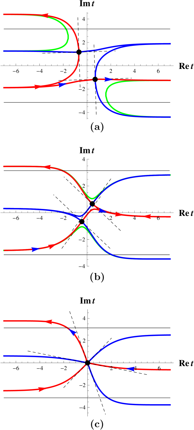
Figure 6: (Color online.) PSD for different values of the argument $z$ and order $\nu$. In (a), $\nu=(1000+1/5){\mathrm{e}}^{{\mathrm{i}}\pi/10}$, $z=(1200+6/25){\mathrm{e}}^{2{\mathrm{i}}\pi/5}$, in (b), $\nu=(1000+1/5){\mathrm{e}}^{{\mathrm{i}}\pi/5}$, $z=(1100+11/50){\mathrm{e}}^{{\mathrm{i}}\pi/10}$, and in (c), $z=\nu=(1000+1/5){\mathrm{e}}^{{\mathrm{i}}\pi/5}$. Red lines show PSDs passing through the saddle points (black dots), blue lines paths of steepest ascent passing through the saddle points. For orientation purposes, thin black lines are drawn at $\operatorname{\textrm{Im}}t=\pm\pi$. Red arrows indicate the integration path to obtain $J_{\nu}(z)$, and blue arrows the paths for $H^{(1)}(z)$ [(a) and (b)] and $H^{(2)}(z)$ [(c)]. In (a) and (b), the green curves are curves satisfying Eq. (66), but not passing through the saddle point. The slopes of the linear segments (71), (78) used in the numerical evaluation are shown with dashed lines. To obtain 10 significant figures, one needs to perform the integration along a linear segment of length approximately equal to the size of the black dots.

A.4 Numerical integration

In terms of the PSD configurations, there are three cases that should be considered separately, depending on the sign of $\operatorname{\textrm{Im}}\left(t_{+}\right)$, where $t_{+}$ is the saddle point with $\operatorname{\textrm{Re}}(t_{+})>0$. The saddle point configuration depends on this sign SmdHTi2009 .

Case 1: If $\operatorname{\textrm{Im}}\left(t_{+}\right)<0$ and consequently $\operatorname{\textrm{Im}}\left(t_{-}\right)>0$, the configuration of the saddle points and PSDs in this case is illustrated in Fig. 6(a). As is gathered from this plot, one saddle point contributes to the value of $J_{\nu}(z)$, and the other to the value of $H_{\nu}^{(1)}(z)$. The remaining function $Y_{\nu}(z)$ can then be computed as $Y_{\nu}(z)=-{\mathrm{i}}[H_{\nu}^{(1)}(z)-J_{\nu}(z)]$. Case 2: If $\operatorname{\textrm{Im}}\left(t_{-}\right)<0$ and therefore $\operatorname{\textrm{Im}}\left(t_{+}\right)>0$, the situation is as shown in Fig. 6(b). To obtain $J_{\nu}(z)$, one has to pass both saddle points, and thus pick up a contribution from both. Case 3: The case $\operatorname{\textrm{Im}}t_{+}=\operatorname{\textrm{Im}}t_{-}=0$ actually needs a separate consideration. It is shown in Fig. 6(c), but only in the special case of coalescing saddle points (see the discussion below). In general, the saddle points may be separated, still, with $\operatorname{\textrm{Im}}t_{+}=\operatorname{\textrm{Im}}t_{-}=0$.

For $\nu\approx z$, but not exact equality, the two saddle points almost coalesce. In Fig. 6(c), we investigate the case $\nu=z$, with $t_{+}=t_{-}=0$. In this case, the saddle point has merged together into a double saddle point at the origin, and $J_{\nu}(z)$ and $H^{(2)}_{\nu}(z)$ are calculated by following the appropriate paths indicated by red and blue arrows, respectively. The linear segment approximation to the true PSD [dashed lines in Fig. 6(c)] are seen to be valid rather far from the saddle point, which implies that the linear approximation to the PSD may be used to good effect. The given linear approximation to the PSD for $\nu=z$ may be used also for the case $\left|1-\frac{\nu}{z}\right|<h$ with given $h$. In practice, the value of $h$ increases with increasing $|z|$, for a given prescribed accuracy of the numerical evaluation. As a rule of thumb, the imaginary part of $g(t)$ along the effective path should be of order 1, where the length of the path is estimated by Eq. (85).

To gain a little more insight into the difficulties associated with the saddle points approaching each other, we discuss the transition from Fig. 6(a) to 6(c), by a suitable change of the parameters. The PSD for $J_{\nu}(z)$ (red arrows) then changes from having smooth curvature at the saddle point [Fig. 6(a)] to having a “kink” at the saddle point [Fig. 6(c)]. Therefore, even if the two saddle points are separated, at some point the linear approximation to the PSD will only hold for a very short segment of the true PSD, and is unsuitable. For some small distance between the saddles, it is instead better to pretend that the suitable contour is given by the double saddle point and to use the dashed lines in Fig. 6(c), even if the saddle points do not exactly coalesce. We illustrate the behavior of the integrand along the approximate PSD when $\nu\approx z$ in Fig. 7. Shown are real and imaginary parts of the integrand $F(\eta)$, where

$$J_{\nu}(z)\approx\int_{\eta_{\textrm{min}}}^{\eta_{\textrm{max}}}F(\eta){\mathrm{d}}\eta,$$ (79)

$$F(\eta)=\frac{1}{2\pi{\mathrm{i}}}{\mathrm{e}}^{g(t(\eta))}\;\frac{{\mathrm{d}}t(\eta)}{{\mathrm{d}}\eta},$$ (80)

and [see Eq. (78)]

$$t(\eta)=\left\{\begin{array}[]{ll}\eta\left[\cot\left(\dfrac{\pi-\arg z}{3}\right)+{\mathrm{i}}\right],&\textrm{if }\eta<0\,,\\ \eta\left[\cot\left(\dfrac{2\pi-\arg z}{3}\right)+{\mathrm{i}}\right],&\textrm{if }\eta\geq 0.\end{array}\right.$$ (81)

In Fig. 7, we have $h=\left|1-\frac{\nu}{z}\right|\approx 3\times 10^{-3}$.

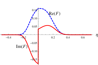
Figure 7: (Color online.) Real (dashed, blue line) and imaginary (red, solid line) parts of the integrand $F(\eta)$ from Eq. (80). The parameter values are $\nu=(500+1/5){\mathrm{e}}^{3{\mathrm{i}}\pi/10}$, and $z=(500+1/10){\mathrm{e}}^{{\mathrm{i}}\pi(3/10+10^{-3})}$. The limits of the $\eta$-axis correspond to those obtained from the estimate (85)

The integration limits for the numerical calculations can be chosen as follows. The primary objective is to estimate how far out from the saddle point the integration should be cut off, that is to estimate the limits $\eta_{\textrm{min}}$ and $\eta_{\textrm{max}}$ in Eq.  (A.3). In the case of separate saddle points, we expand $g(t)$ around the saddle point up to second order, to obtain an integral of the form

$$I_{1}(X)=\int_{0}^{X}{\mathrm{e}}^{-C_{1}s^{2}}{\mathrm{d}}s\,,$$ (82)

where $X$ and $C_{1}$ are positive real constants. It follows that if we want relative precision $\epsilon=|1-I_{1}(X)/I_{1}(\infty)|$ we must cut the integral at

$$X=\frac{\operatorname{erfc}^{-1}(\epsilon)}{\sqrt{C_{1}}},$$ (83)

where $\operatorname{erfc}^{-1}(\cdot)$ is the inverse of the complementary error function. For coalescing saddle points, also the second derivative of $g(t)$ vanishes, and we must instead consider integrals like

$$I_{2}(X)=\int_{0}^{X}{\mathrm{e}}^{-C_{2}s^{3}}{\mathrm{d}}s.$$ (84)

Here, we should cut at

$$X=\left[\frac{\Gamma^{-1}(\frac{1}{3},\epsilon)}{C_{2}}\right]^{\frac{1}{3}},$$ (85)

to obtain a prescribed precision $\epsilon$. In Eq. (85), $\Gamma^{-1}(\cdot,\cdot)$ is the inverse of the incomplete gamma function with respect to its second argument. These estimates assumes a monotonically decreasing integrand along the path of steepest descent, and it is clear that it is impossible to reach arbitrary precision due to incurred oscillations along the linear line segments approximating the paths of steepest descent, as one travels too far from the saddle point.

In Ref. SmdHTi2009 , the authors also advocate to use an approximation of the saddle point contour by linear line segments. They first observe that it is possible to solve the PSD equation (66) numerically, but then show that if oscillations do not induce prohibitive numerical instability, equally accurate results may be obtained by just taking line segments. Because it is time-consuming to calculate the PSD numerically, they conclude that the line-segment approach should be favored. However, as mentioned previously, this approach necessarily breaks down at some level of precision, especially for large values of $|z|$. To reach (in principle) arbitrary precision for large magnitudes of the order and argument with the saddle point method, it seems unavoidable to follow the true PSD as closely as possible.

An optimized, hybrid algorithm should perform the PSD stepping and the integration in parallel: First, one advances on the PSD by one step, computes the integral on the segment connecting the previous point by the new point, checks if the accuracy demand is satisfied, if not, one takes another step. The step length could be adjusted according to how close the condition $\operatorname{\textrm{Im}}(g(t_{\pm}))=\operatorname{\textrm{Im}}(g(t))$ is satisfied. Since the integrand decreases exponentially along the PSD, and does not oscillate, it should be straightforward to estimate when to stop the stepping/integration. Still, for this algorithm to be universally applicable, it might be necessary to investigate the overlap regions where the saddle-point configurations versus the double saddle point configurations should be used, and to develop special routines that deal with the line segments joining the two saddle points in overlapping regions. We have not pursued this endeavor any further in the current work and leave it as an open problem.

References

- (1) P. Debye, Math. Ann. 68, 535 (1909).
- (2) J. R. Airy, Phil. Mag. 31, 520 (1916).
- (3) J. W. Nicholson, Phil. Mag. 19, 247 (1910).
- (4) G. N. Watson, Proc. Camb. Phil. Soc. 19, 96 (1918).
- (5) R. E. Langer, Trans. Amer. Math. Soc. 33, 23 (1931).
- (6) R. E. Langer, Trans. Amer. Math. Soc. 34, 447 (1932).
- (7) R. E. Langer, Trans. Amer. Math. Soc. 67, 461 (1949).
- (8) T. M. Cherry, J. London Math. Soc. 24, 121 (1949).
- (9) T. M. Cherry, Trans. Amer. Math. Soc. 68, 224 (1950).
- (10) R. Grimshaw, J. Austral. Math. Soc. Ser. B 30, 378 (1989).
- (11) G. N. Watson, A Treatise on the Theory of Bessel Functions (Cambridge University Press, Cambridge, UK, 1922).
- (12) M. Abramowitz and I. A. Stegun, Handbook of Mathematical Functions, 10 ed. (National Bureau of Standards, Washington, D. C., 1972).
- (13) F. W. J. Olver, D. W. Lozier, R. F. Boisvert, and C. W. Clark, NIST Handbook of Mathematical Functions (Cambridge University Press, Cambridge, 2010).
- (14) A wide variety of useful formulas concerning special functions is digitally available at http://dlmf.nist.gov.
- (15) P. J. Mohr and P. Indelicato, J. Math. Phys. 36, 714 (1995).
- (16) O. Vallée and M. Soares, Airy Functions and Applications to Physics (World Scientific, Singapore, 2010).
- (17) A. Cuyt, P. V. Brevik, B. Verdonk, H. Waadeland, and W. B. Jones, Handbook of Continued Fractions for Special Functions (Springer, New York, 2008).
- (18) A. Gil, J. Segura, and N. M. Temme, Numerical methods for special functions (Society of Industrial Applied Mathematics, Philadelphia, PA, 2007).
- (19) N. M. Temme, Acta Numer. 16, 379 (2007).
- (20) A. Gil, J. Segura, and N. M. Temme, in Recent Advances in Computational and Applied Mathematics, edited by T. E. Simos (Springer, Dordrecht, 2011), pp. 67–121.
- (21) F. W. J. Olver, Phil. Trans. R. Soc. Lond. A 247, 307 (1954).
- (22) F. W. J. Olver, Phil. Trans. R. Soc. Lond. A 247, 328 (1954).
- (23) F. W. J. Olver, Asymptotics and Special Functions (Academic Press, New York, NY, 1974); reprinted as AKP Classics (A. K. Peters Ltd., Wellesley, MA, 1997).
- (24) E. Caliceti, M. Meyer-Hermann, P. Ribeca, A. Surzhykov, and U. D. Jentschura, Phys. Rep. 446, 1 (2007).
- (25) C. B. Balogh, Bull. Amer. Math. Soc. 72, 40 (1966).
- (26) Z. Schulten, D. G. M. Anderson, and R. G. Gordon, J. Comp. Phys. 31, 60 (1979).
- (27) N. M. Temme, Proceedings of Symposia in Applied Mathematics 46, 395 (1994).
- (28) N. M. Temme, Numer. Algor. 15, 207 (1997).
- (29) C. J. Howls and A. B. Old Daalhuis, Proc. Roy. Soc. London A 455, 3917 (1999).
- (30) R. B. Paris, Proc. Roy. Soc. London A 457, 2835 (2001).
- (31) R. B. Paris, Proc. Roy. Soc. London A 457, 2855 (2001).
- (32) R. B. Paris, Proc. Roy. Soc. London A 460, 2737 (2004).
- (33) W. Shi and R. Wong, Asymptotic Analysis 63, 101 (2009).
- (34) R. W. Smink, B. P. de Hon, and A. G. Tijhuis, Appl. Math. Comput. 207, 442 (2009).
- (35) D. Baruth, A numerical algorithm, based on the Debye expansion, can be found on web pages by D. Baruth, see http://www.iging.com/transcendental/J_1000000.htm. The algorithm is designed to calculate Bessel functions of large orders and arguments.
- (36) B. R. Fabijonas, D. W. Lozier, and F. W. J. Olver, ACM Trans. Math. Soft. 30, 471 (2004).
- (37) P. J. Mohr, Ann. Phys. (N.Y.) 88, 26 (1974).
- (38) P. J. Mohr, Ann. Phys. (N.Y.) 88, 52 (1974).
- (39) E. Lötstedt and U. D. Jentschura, Phys. Rev. E 79, 026707 (2009).
- (40) J. C. P. Miller, Quart. J. Mech. Appl. Math. 3, 225 (1950).
- (41) W. G. Bickley, L. J. Comrie, J. C. P. Miller, D. H. Sadler, and A. J. Thompson, Bessel functions, Part II, functions of positive integer order, vol. X of Mathematical tables (Cambridge University Press, Cambridge, 1960).
- (42) W. Gautschi, SIAM Rev. 9, 24 (1967).
- (43) E. J. Weniger, Comput. Phys. Rep. 10, 189 (1989).
- (44) E. J. Weniger, Appl. Numer. Math. 60, 1429 (2010).
- (45) E. J. Weniger, Comput. Phys. 10, 496 (1996).
- (46) S. Wolfram, Mathematica-A System for Doing Mathematics by Computer (Addison-Wesley, Reading, MA, 1988).
- (47) U. D. Jentschura, P. J. Mohr, and G. Soff, Phys. Rev. Lett. 82, 53 (1999).
- (48) U. D. Jentschura, P. J. Mohr, and G. Soff, Phys. Rev. A 63, 042512 (2001).
- (49) U. D. Jentschura, P. J. Mohr, G. Soff, and E. J. Weniger, Comput. Phys. Commun. 116, 28 (1999).
- (50) J. D. Jackson, Classical Electrodynamics, 3 ed. (J. Wiley & Sons, New York, NY, 1998).
- (51) G. Matviyenko, Appl. Comput. Harm. Anal. 1, 116 (1993).