Folding a protein with equal probability of being helix or hairpin

Abstract

We explore the possibility for the native state of a protein being inherently a multi-conformation state in an ab initio coarse-grained model. Based on the Wang-Landau algorithm, the complete free energy landscape for the designed sequence 2D4X: INYWLAHAKAGYIVHWTA is constructed. It is shown that 2DX4 possesses two nearly degenerate native states: one has a helix structure, while the other has a hairpin structure and their energy difference is less than 2% of that of local minimums. Two degenerate native states are stabilized by an energy barrier of the order 10kcal/mol. Furthermore, the hydrogen-bond and dipole-dipole interactions are found to be two major competing interactions in transforming one conformation into the other. Our results indicate that degenerate native states are stabilized by subtle balance between different interactions in proteins; furthermore, for small proteins, degeneracy only happens for proteins of sizes being around 18 amino acids or 40 amino acids. These results provide important clues to the study of native structures of proteins.

Key words: Wang-Landau algorithm 1; $\alpha$-$\beta$ transition 2; coarse grained model 3

Introduction

Solving the protein folding problem has tremendous implications. Among possible applications, the solution to the problem makes it possible to design drugs theoretically, which would result in the greatest impact to the biological science. Nonetheless, despite much effort being devoted during the past, the problem continues to be one of the most basic unsolved problems. To solve the folding problem completely, it is generally believed that to be able to predict the protein structure for a given sequence of amino acids is an important step. This belief originates from the classical Anfinsen’s work (1) and is often summarized by stating that there is a unique native configuration for a given sequence of amino acids. Over the past decades, this point of view, however, has been challenged by experimental evidences. It is now known that proteins can be driven to different folded states by changing pH value, ionic strength (2, 3), temperature (4), or solvent polarity (5). These facts indicate that there may exit nearby competing states to the native state of globular proteins in vivo. Therefore, given appropriate conditions, the native state of a given sequence of amino acids can be changed. In particular, it implies that the structure of a given segment of amino acids may depend on the context it resides in.

Indeed, accumulating evidences have indicated that the secondary structure can be context dependent. Bovine $\beta$-lactoglobulin protein is a predominantly $\beta$-sheet protein but it has been observed to go through a remarkable $\alpha$ to $\beta$ transition during the folding process (6, 7). Kabsch and Sander also found a pentapeptide sequence which could adopt an $\alpha$-helical or a $\beta$-sheet conformation in different proteins. Cohen and colleagues (8) extended this work to hexapeptides. Minor and Kim (9) have conducted an experiment showing that an 11 amino acid sequence can be transformed into an $\alpha$-helical or a $\beta$-sheet in protein G. Such ’chameleon’ sequences have their cooperative local interactions competing against long range interactions of sequence environment. The fragmental propensity of secondary structures are found to be overwhelmed by larger structures.

To elucidate the mechanism that causes the conformation change, a de novo protein has recently been designed (10). The modified sequence INYWLAHAKAGYIVHWTA posited in Protein Data Bank (11) (PDB ID 2DX3 and 2DX4, and we shall term it simply as 2DX4 hereafter) from residues 101-111 of human $\alpha$-lactalbumin was identified to has equal population of $\alpha$-helical or $\beta$-sheet in an aqueous solution. Although it is well recognized that protein solutions are in equilibrium with intermediate peptides, the dual native states are rarely reported in the literature. Furthermore, it is shown that the conformational transformation of 2DX4 is not induced by any environmental conditions or binding motifs. These facts make 2DX4 a valuable target to study. In particular, folding 2DX4 would be a crucial test for any viable approach for solving the protein folding problem.

On the theoretical side, although all-atom simulation is the most comprehensive approach for understanding the folding processes; nonetheless, the requirement of computational resources tends to be realistically unaffordable (12). Itoh, Tamura and Okamoto (13) have combined all-atom molecular dynamics simulation with multi-canonical multioverlap algorithm to simulate 2DX4. From the limited phase space obtained, they investigated possible pathways for the $\alpha$ to $\beta$ transition. In particular, three local minima in free energy are identified. However, only partial $\alpha$ helix or $\beta$ hairpin are found in the structures associated with these local minima. The mechanism that is responsible for the possibility of two native states of 2DX4 thus remains unclear. On the other hand, there have been much effort in developing coarse grained models to predict protein structures (14). In these models, effects of water molecules are implicitly included in effective interacting potentials between amino acids. The required computational resources is much reduced and it enables the prediction of protein structures feasible. Indeed, progress have recently been made in predicting structures of wild-type proteins of sizes from 12 to 56 amino acids by using realistic and unbiased potentials between amino acids (15). To further check the validity of coarse grained models, folding proteins such as 2DX4 would be an ideal test.

In this work, based on the ab initio coarse-grained model constructed in Ref. (15), we constructed the complete free energy landscape for 2DX4. It is shown that in agreement with the experimental observation, there are only two local minima with structures being $\alpha$-helix and $\beta$-hairpin respectively. Moreover, within the accuracy of the coarse-grained model, it is found that while two local minima are degenerate in the case of 2DX4, the $\beta$-hairpin is higher in energy for the DP3 protein which results from the mutation of one amino acid of 2DX4 and was reported to have zero population of hairpin structure (10). In addition, the pathways between the helix and hairpin configurations are simulated by Monte Carlo (MC) algorithm in high temperatures. By analyzing detailed free energy profile, we find that the hydrogen-bond and dipole-dipole interactions are two major competing mechanism in transforming one conformation into the other. Our results indicate that generally, degenerate native states are stabilized by subtle balance between different interactions in proteins. Furthermore, for small proteins, degenerate native states only happen for proteins of sizes being around 18 amino acids or 40 amino acids. These results provide important clues to the study of native structures of proteins.

Theory and Methods

Ab Initio Coarse-grained Potentials

We shall first recapture essentials of the coarse-grained model constructed in Ref. (15). In this model, residues are coarse-grained as spheres centered at $\rm{C}^{\beta}$ atoms but complete structures are kept in backbones. Bond angles and bond lengths are fixed between these atoms to increase folding efficiency, the only variables are dihedral angles $\phi$ and $\psi$ on the $\rm{C}^{\alpha}$ atom hinging two amide planes. On the other hand, water molecules are not included explicitly but their effects are incorporated in effective potentials among side-chains and backbones. In these representations and with all energies being in unit of kcal/mol, the total energy can be written as

$$E_{total}=E_{Steric}+E_{DD}+E_{HB}+E_{MJ}+E_{NP}+E_{SA}.$$ (1)

Here each energy term is a weighted potential energy with $E_{i}=\varepsilon_{i}V_{i}$ , where $\varepsilon_{i}$ is the weighting factor to be determined later and $V_{i}$ is the corresponding potential energy. Among these energy terms, $E_{Steric}$ is to enforce the structural constraints such as hard-core potentials to avoid unphysical contacts, while $E_{SA}$ is solvent accessible surface energy in proportional to the area of each side-chain that is exposed to water and is primarily responsible for stabilizing the tertiary structure. The remaining terms are three ingredients for the formation of the secondary structures with $E_{HB}$ being the hydrogen bonding between any non-neighboring $NH$ and $CO$ pair, $E_{DD}$ being the summation of screened dipole-dipole interaction at large distance (global dipole interaction, $E_{DG}$) and local dipole-dipole interaction between dipoles on the backbones, and $E_{MJ}+E_{NP}$ accounting for the interactions due to hydrophobicity or the charge state of the amino acids. All the potentials were based on realistic parameters obtained from experimental data except for $E_{MJ}+E_{NP}$, which was based simple generalizations of Miyazawa-Jernigan matrix (16, 17) by using 12-6 Lennard-Jones potential modified by effects due to sizes of water molecules (15). In order to include realistic effects due to hydrophobicity or the charge state of the amino acids, we shall construct the corresponding potentials by statistical methods so that $E_{MJ}$ generalizes Miyazawa-Jernigan Matrix (16, 17) to finite large distances between amino acids, while $E_{NP}$ generalizes the $V_{LocalHP}$ in Ref. (15) and is the statistical energy that characterizes the propensity (to $\alpha$ or $\beta$) of amino acids in nearest neighbors. With these potentials, the weighting factors $\epsilon_{i}$’s are calibrated based on a few proteins of known structures (15). Their values are $\varepsilon_{DG}$ =0.21, $\varepsilon_{DN}$ = 2.0, $\varepsilon_{HB}$ = 4.8, $\varepsilon_{SA}$ = 1.35, and $\varepsilon_{MJ}$ = 0.85; while for helix and sheet propensity energies, we get $\varepsilon_{NP}^{\alpha}$ = 6.4 and $\varepsilon_{NP}^{\beta}$ = 16,

To extend the Miyazawa-Jernigan Matrix to finite distances, we perform extended statistical analysis by first writing

$$E_{MJ}=\varepsilon_{MJ}\sum_{i,j}V_{ij;MJ}(r)(1-SA_{i})(1-SA_{j}),$$ (2)

where $SA_{i}$ and $SA_{j}$ are the solvent accessibilities for $i$th and $j$th residue respectively. The quantity, $V_{ij;MJ}(r)$, is the statistical potential between the $i$th and $j$th residues obtained by counting number $n_{ij}$, of the corresponding $i$-type and $j$-type residues separating by $r$, that appears in the PDB. Fundamentally, $V_{ij;MJ}(r)$ is the generalization of the pair distribution function (18) and its relation to $n_{ij}(r)$ is given by the Boltzmann’s statistics

$$\exp(-V_{ij;MJ}(r))=A(r_{k})\frac{\sum\limits_{p}n_{ij;p}(r_{k})}{\sum\limits_{p,r_{k}}\frac{\displaystyle(n_{ir;p}(r_{k})+n_{i0;p}(r_{k}))(n_{jr;p}(r_{k})+n_{j0;p}(r_{k}))}{\displaystyle(n_{rr;p}(r_{k})+n_{r0;p}(r_{k}))}},$$ (3)

where $A(r_{k})$ is a normalization factor to be determined later, numbers with the index $p$ denote the corresponding statistical values that belong to one specific protein $p$, $0$ represents the solvent group, and $r_{k}$ is the radius of the kth spherical shell centered at $i$-type residue. Note that different amino acids have different occurrence frequency in real proteins and this is normalized by the denominator in Eq.3. Furthermore, homology of sequence bias was eliminated by the sequence alignment method in combination with the weighting matrix used by Miyazawa and Jernigan (17). Here 2$n_{ij}(r_{k})$ for i $\neq$ j and $n_{ii}(r_{k})$ are the counts when the $i$-type residue is at the origin and the $j$-type residue is in the kth distance $r_{k}$, while $n_{ir}$ is the total count of the $i$the residue

$$n_{ir;p}(r_{k})=\sum\limits_{j}n_{ij;p}(r_{k}).$$ (4)

$n_{i0}$ counts events taking place between the $i$-type residue and solvent group 0

$$n_{i0;p}(r_{k})=\frac{1}{2}q_{i}(r_{k})n_{i;p}(r_{k})-n_{ir;p}(r_{k}),$$ (5)

where $q_{i}$ is the coordinate number of the $i$-type residue in the $k$th spherical shell and $n_{i}$ is the total number of the $i$-type residues in protein $p$. $n_{rr}$ and $n_{r0}$ are summations of $n_{ir}$ and $n_{i0}$ over $i$-type residue respectively

$$n_{rr;p}(r_{k})=\sum\limits_{i}n_{ir;p}(r_{k}),$$ (6)

$$n_{0r;p}(r_{k})=\sum\limits_{i}n_{i0;p}(r_{k}).$$ (7)

Finally, the normalization factor A(r) is defined by

$$A(r_{k})=\frac{{\rm total\hskip 2.0ptnumber\hskip 2.0ptof\hskip 2.0ptshells}}{\frac{4}{3}\pi[(r_{k}+\frac{\Delta r}{2})^{3}-(r_{k}-\frac{\Delta r}{2})^{3}]},$$ (8)

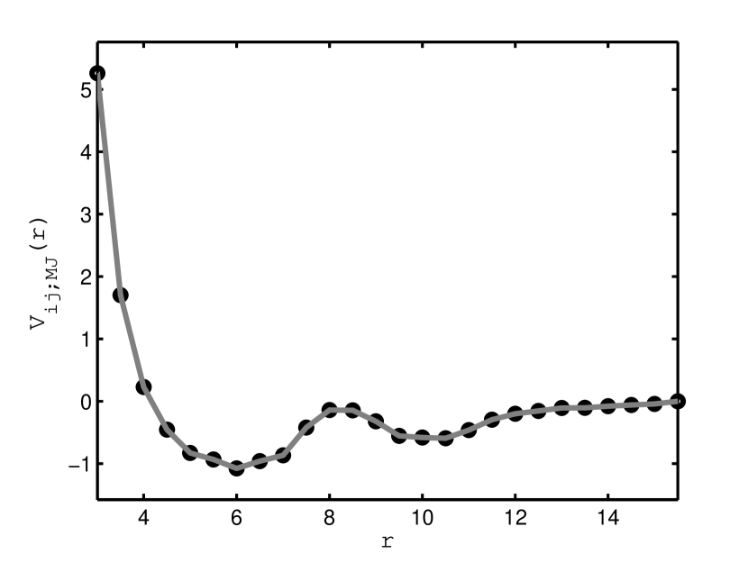
where $\Delta r$ is the width of each spherical shell. The effective potential as a continuous function of $r$, $V_{ij;MJ}(r)$, is then interpolated from $V_{ij;MJ}(r_{k})$. As a demonstration, in Fig. 1 , we show a typical effective potential obtained by the above statistical analysis. We see that similar to the pair distribution function for liquid molecules (18), $V_{ij;MJ}(r)$ exhibits similar oscillations in consistent with the desolvation model (19). Furthermore, even though there are structures in proteins, there is no indication of any ordering in $V_{ij;MJ}(r)$.

The effective $V_{ij;MJ}(r)$ is only valid for large enough distances. For residues in nearest neighbors, due to the steric constraints, the pair distribution function starts to deviate from the desolvation model. To extend $E_{MJ}$ to characterize interactions of residues in nearest neighbors, $E_{NP}$ is introduced to account for the statistical energy between nearest neighboring residues. The interactions among nearest neighboring residues are best characterized by dihedral angles $\phi$ and $\psi$ of the corresponding amide planes. Since $V_{ij;MJ}(r)$ does not cover distances of three successive residues, $E_{NP}$ needs to characterize three successive residues in the protein, labeled by $i-1$, $i$, and $i+1$. Using the corresponding dihedral angles shown in Fig. 2 , $E_{NP}$ can be written as

$$E_{NP}=\sum\limits_{i}\sum\limits_{k=\alpha,\beta}\varepsilon_{NP}^{k}[V_{lm}^{k}(\psi_{i-1},\phi_{i})+V_{mn}^{k}(\psi_{i},\phi_{i+1})]V_{m}(\phi_{i},\psi_{i}),$$ (9)

where $l$, $m$ and $n$ are indices for type of residues, $V_{m}$ is a one-body potential that depends on $\psi_{i}$ and $\phi_{i}$ of the amide planes connecting to the $m$-type residue, and $V_{lm}$ (also $V_{mn}$) is a two-body energy that depends dihedral angles of $l$-type and $m$-type residues in nearest neighbors. According to the Ramachandran plot, it is known that $\phi$ and $\psi$ are statistically concentrated at particular regions, which are either in the $\alpha$-helix configuration or $\beta$-sheet configuration. To ensure the relative magnitudes of $\alpha$-helix and $\beta$-sheet part are not biased by the database, different weighting factors with $k=\alpha$ and $\beta$ are introduced in Eq. 9.

The one-body angular potential $V_{m}$ is obtained by first analyzing the bare potential $v_{m}$ defined by

$$\exp(-v_{m}(\phi,\psi))=\frac{n_{m}(\phi,\psi)}{\int\int n_{m}(\phi,\psi)d\phi d\psi},$$ (10)

where $n_{m}$ is the number density taken over the whole PDB for type $m$ residues with dihedral angles being $(\phi,\psi)$. To account for the preference or non-preference of $\alpha$ or $\beta$ structures, we set $V_{m}(\phi_{i},\psi_{i})=\theta(\Lambda-v_{m}(\phi_{i},\psi_{i}))$ with $\theta$ being the step function and $\Lambda$ being a negative threshold energy level so that $V_{m}$ is either $1$ or $0$.

The bare two-body potential is constructed by

$$\exp(-v_{lm}^{k}(\psi_{i-1},\phi_{i}))=\frac{n_{lm}(\psi_{i-1},\phi_{i})\int\int n_{rr}(\psi_{i-1},\phi_{i})d\psi_{i-1}d\phi_{i}}{\int\int n_{lr}(\psi_{i-1},\phi_{i})d\psi_{i-1}d\phi_{i}\int\int n_{mr}(\psi_{i-1},\phi_{i})d\psi_{i-1}d\phi_{i}},$$ (11)

where $n_{lr}$, $n_{mr}$ and $n_{rr}$ are defined in same way as those in Eq. 4 and Eq. 6 except that they are specialized to the dihedral angle $(\psi_{i-1},\phi_{i})$. $V_{lm}^{k}(\psi_{i-1},\phi_{i})$ is then defined by rescaling $v_{lm}$ with respect to the average value of $v_{lm}$

$$V_{lm}^{k}(\psi_{i-1},\phi_{i})=(A_{lm}^{k}-A_{ave}^{k})v_{lm}^{k}(\psi_{i-1},\phi_{i})/A_{lm}^{k}$$ (12)

where $A_{lm}$ is the minimum of $v_{lm}$ over all possible $(\psi_{i-1},\phi_{i})$ and $A_{ave}$ is the average value of $A_{lm}$ over all possible pairs of amino acids. A typical $V_{lm}$ is shown in Fig. 2 . It is clear that $V_{i-1,i}(\psi_{i-1},\phi_{i})$ does not vanish only in particular regions, in which local structures of proteins are either $\alpha$ helices or $\beta$ sheets.

Wang-Landau Monte Carlo algorithm

Given the ab initio coarse-grained potential obtained, one can determine the free energy landscape by using the Wang-Landau algorithm (20). The density of states is estimated by random sampling on energy space via the transition probability

$$P(E_{1}\rightarrow E_{2})=\min(\frac{g(E_{1})}{g(E_{2})},1),$$ (13)

where $g(E)$ is the density function of energy E. Although this algorithm was first demonstrated on Ising model of spin array, it is portable to molecular systems with continuous energy value (21, 22). Specific implementations adapted in our work are the following steps:
(1) Define a density function g(E, X) and histogram H(E, X) with X’s being any variables other than energy. Set initial values: g(E,X) = 1 and H(E, X) = 0 for all E and X.
(2) Generate an initial conformation randomly and calculate its energy $E_{1}$.
(3) Generate a new conformation by making a small change (e.g. the dihedral angles). Calculate the new energy $E_{2}$ and the transition to the new conformation is determined by the transition probability $P(E_{1},X_{1}\rightarrow E_{2},X_{2})=\min[g(E_{1},X_{1})/g(E_{2},X_{2}),1]$.
(4) If the system stays in the original $E_{1}$ state, $g(E_{1},X_{1})$ is replaced by $g(E_{1},X_{1})\times f$ and $H(E,X)$ is accumulated through $H(E_{1},X_{1})+1$. Otherwise, one sets $g(E_{2},X_{2})=g(E_{2},X_{2})\times f$ and $H(E_{2},X_{2})=H(E_{2},X_{2})+1$. The factor f is initially set to $e^{1}$.
(5) After each MC step, check if less than 2 % of sites in $H$ are smaller than flat threshold, which is defined to be 10 % of averaged $H(E,X)$. If this is satisfied, the histogram is flat and one then sets $f=\sqrt{f},H(E,X)=0$ and goes to step (2). When $f<\exp(10^{-3.6})$ is satisfied, one exists the procedure.

All the above steps are identical to Wang-Landau’s scheme except for the flat histogram criteria in step (5), which is modified to accommodate enormous states involved for proteins so that sampling can be done in finite computation time. Once the density of states is constructed, the free energy landscape can be calculated as

$$F(E,X)=E-k_{B}T\log[g(E,X)],$$ (14)

where $k_{B}$ is the Boltzmann constant and $T$ is the absolute temperature. The variable space X is not restricted to be one dimension and has to be chosen to exhibit the landscape.

Results

Propensity Analysis and Monte Carlo Simulation

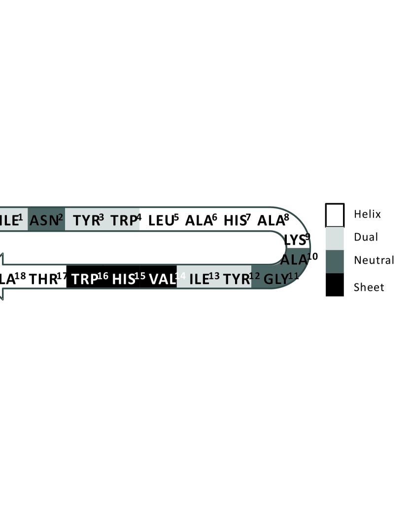
To investigate the energy landscape of 2DX4, we first analyze its propensity. Past studies (23, 24) have indicated that each amino acid has its propensity of secondary structure. By using the constructed statistical potential $V_{lm}$ (see Theory and Methods), we summarize the nearest neighbor propensity of 2DX4 in Fig. 3. Here amino acids in nearest neighbors are classified according to the tendency of corresponding amino acids being in $\alpha$-helix, $\beta$-sheet, dual or neutral. The dual propensity implies the residue pair can adopt either $\alpha$ or $\beta$ structure. By contrast, the neutral propensity implies that the residue pair is free to rotate in dihedral angles and it is often that a turn region of anti-parallel $\beta$-sheet is developed. From the propensity analysis, it is clear that even though there is no absolute global tendency for 2DX4 being $\alpha$ helix or $\beta$ sheet, by including residues with neutral and dual propensities, there are more residues in favor of $\alpha$ helix. Nonetheless, the high $\beta$-sheet propensity near the C-terminal, containing amino acids V, H, and W, indicates the possibility of switching 2DX4 between helix and hairpin structures. Since each of these three amino acids has larger side chain radius than the averaged radius of others, it is more difficult for the segment to curl into part of the helix structure. As a result, the strand formed by residues 14-18 regularly dangles in solvent and deposits a nucleation seed to transform from $\alpha$-helix to $\beta$-sheet.

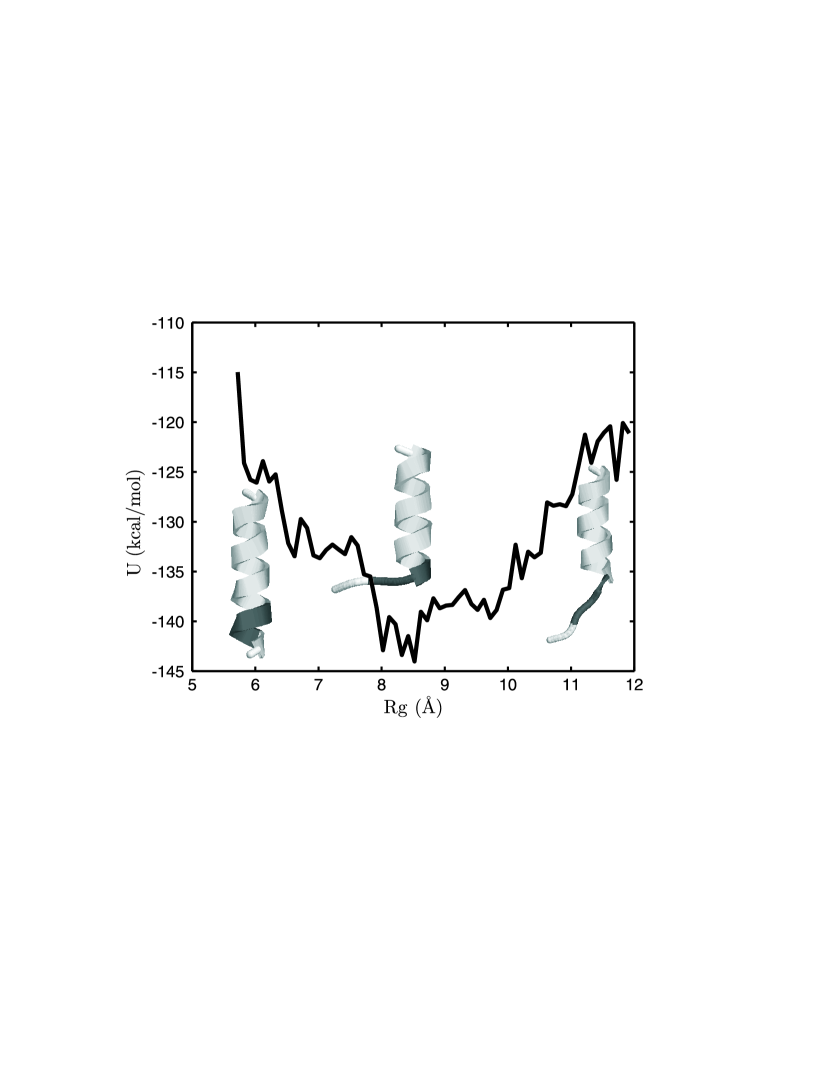
In order to investigate the stability of $\alpha$ helix due to residue 14-18, a MC simulation of 2DX4 by starting from an all helix conformation is conducted. Since the expanding of the strand affect the size of 2DX4, we record the radius of gyration ($Rg$) for structure resembling the $\alpha$-helix. Larger $Rg$ represents structures with extended strands, while smaller $Rg$ represents structures which are closer to the standard $\alpha$-helix. Since each $Rg$ interval may contains several helix structures with different energy values, the internal energy $U$, defined by the Boltzmann statistics $U=\sum_{E}E\exp(-\beta E)$, is evaluated as a function of Rg. In Fig. 4, we show the plot of $U$ versus $Rg$. It is seen that the lowest energy state is not a complete $\alpha$ helix. In general, hydrogen bonds and long range dipole energy favor helix structures (15). In the case of 2DX4, nearest neighbor interactions $V_{NP}$ compete with these helix-favored energies and result in the lowest total energy state with partial helix and partial strand structure. The native structure found in our MC simulation is identical to results obtained by the experiment (10) and other simulations (13), indicating the credibility of the coarse-grained potentials described in Eq. 1.

To clarify the final fate of $\alpha$ helix, we perform full MC simulations by starting from the initial state of a straight line with all dihedral angles $\phi$ and $\psi$ being equal to 180 degree. Indeed, two configurations of lowest energies are found and correspond to $\alpha$ helix and $\beta$ hairpin with RMSD (root mean square deviation of positions) being 3.74 ${\AA}$ and 4.40 ${\AA}$ respectively. The simulations take $4\times 10^{8}$ MC steps and ended on either helix or hairpin states. Furthermore, starting from an $\alpha$ helix at 400 K (RT = 0.8 kcal/mol), the $\alpha$ helix is transformed into a $\beta$ sheet and vice versa. All of the transitions occurred successfully in our MC simulations. However, the helix to hairpin transition takes twice to ten times of more MC steps than that for the transition from hairpin to the helix. A hairpin to helix transition finished approximately in $5\times 10^{7}$ MC steps, where the reverse process took $10^{8}$ MC steps or longer. The obtained asymmetry of transition rates are consistent with the literature report (25), where progress of $\beta$-hairpin formation is thirty times slower than the rate of $\alpha$-helix.

Free Energy Landscape

In order to make sure if helix and hairpin structures found in MC simulations are the only two minimum, we calculate the free energy by employing the Wang-Landau algorithm. In addition to the energy, we characterize the energy landscape by using the contact ratio $Q$ as another coordinate. Here $Q$ is defined by using the conformation of the minimum state with helical like structure as the reference state so that $Q$ is the ratio of contact number of the state to that of the minimum state. The free energy $F$ is thus a function of energy $E$ from -150 kcal/mol to 0 kcal/mol and contact ratio Q, ranging from 0 to 1. In the calculation, to insure that all regions can be accessed, a trial run with $4\times 10^{8}$ MC steps is first performed to identify regions with scarce probability. In the latter runs, free energy density in these regions will be computed separately.

Figure 5 shows the resulting complete free energy landscape for 2DX4. It demonstrates that the free energy has only two minimum at helix and hairpin states. The difference of free energies for helix and hairpin structures is less than 0.17 kcal/mol at room temperature, which clearly demonstrates that 2DX4 is a two-state protein with two stable native states. In Fig. 5, the one-dimensional free energy curves $F(Q)$ are deduced from the density of states $g(E,Q)$ via the formula $\exp(-F(Q)/KT)=\sum_{E}g(E,Q)\exp(-E/KT)$. A free-energy barrier around 10 kcal/mol exists between helix and hairpin structures, Since the energy barrier is much larger than typical energy fluctations $k_{B}T$, it stabilizes both helix and hairpin. The free energy landscape also depends on temperature. At temperature $k_{B}T=0.8$, about 400 K, the minimum at helix side expands from $Q=1$ to $Q=0.65$ with residues 1-10 being kept in helix conformation. In other words, half of the peptide on N-terminal is thermally stable in helix, and residues 11-14 are free to denature at high temperatures.

As a comparison, we examine energy landscapes of mutated 2DX4 through Y12S mutation, which are labeled as DP3 and DP5 in the previous experiment (10). It is reported that DP3 has zero population of hairpin formation in the sense that even though there is minor intra-strand signal, there is no inter-strand signal for the hairpin structure. It is therefore important to examine native states of DP3 in the current model. Figure 5 reveals that for DP3, helix region gets expanded, while hairpin region gets shrunk. This indicates that helix structure is more stable for DP3. Indeed, Fig. 5 shows that the free energy of the helix state is less than that of the hairpin state by 1.1 kcal/mol at room temperature. In addition, we find that this energy difference is sensitive to temperature and becomes 1.4 kcal/mol at 100 K. In contrast, for DP5, the free energy of the helix state is found to be fixed at 100-298K, suggesting that helical structure is thermally more stable in DP5 than in DP3, in agreement with experimental observation (10). Note that it is presumed (10) that absence of $\pi$-$\pi$ interaction of Tyr12-His7 near the turn region is the cause for the absent of hairpin in DP3. However, close examination based on the propensity indicates that mutation of Y12S in DP3 intensify the $\beta$ sheet propensity of the second strand. Thus the lack of hairpin population in DP3 is due to inter-strand interactions not intra-strand propensity. These results are consistent with experimental results that DP3 has only intra-strand signal. The rigidity of second strand and absent of one $\pi$-$\pi$ bond are thus responsible for unstable helix as well as zero population of hairpin in DP3.

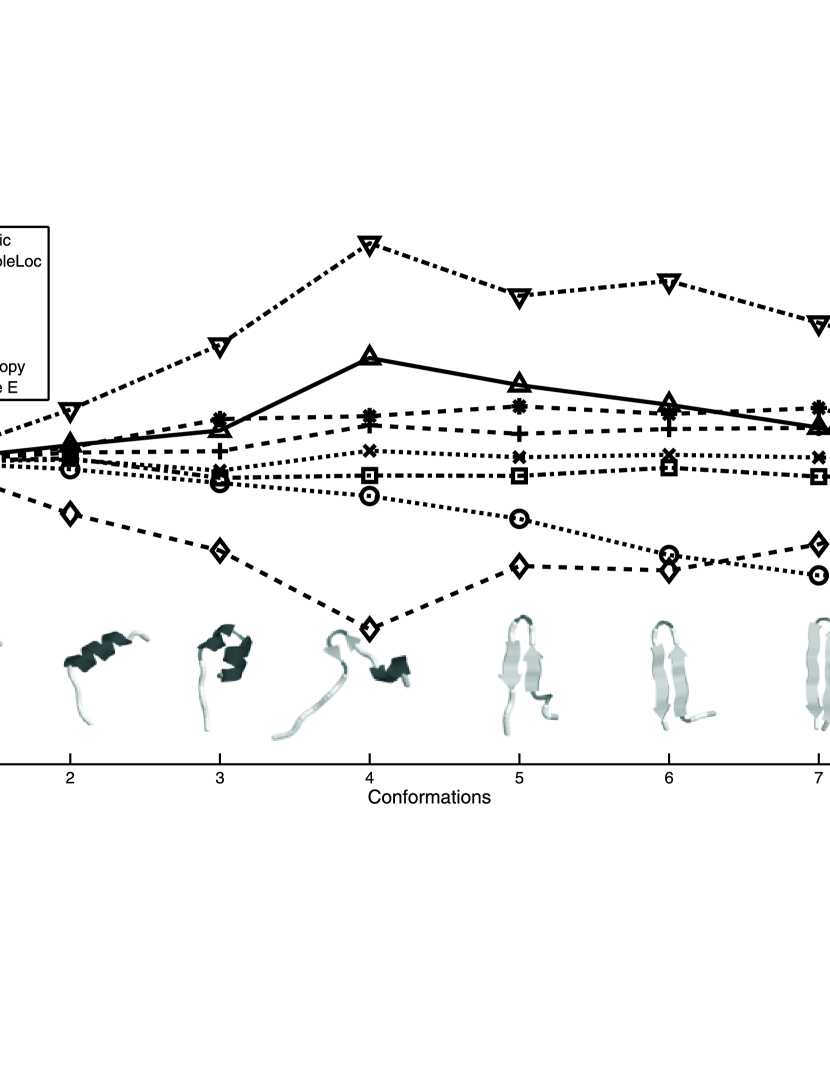
The mechanism for the existence of degenerate native states can be explored by analyzing changes of different energy terms when 2DX4 changes between the helix and the hairpin structures. Figure 6 shows changes of different energies on the path between the helix and the hairpin structures. We find that the degeneracy is due to a large compensation between hydrogen bond energy (HB) and local dipole energy. Physically, it is known that the helix structure has more hydrogen bonds (15) and hence one looses energy in hydrogen bonds by going from the helix structure to the hairpin structure. On the other hand, $\beta$ sheets contain large anti-parallel dipoles on nearest neighboring amide planes, which lowers down the local dipole interaction energy. Differences of other energy terms in 2DX4 are around 2-3 kcal/mol. Therefore, our results show that the compensation of these two energy leads to the degeneracy of the helix and hairpin structures.

Discussion and Conclusion

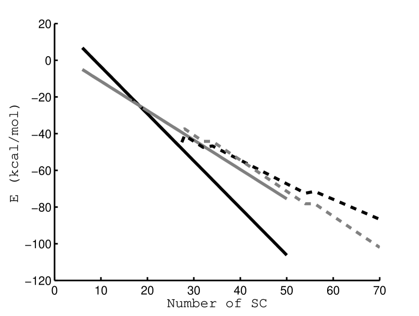
In summary, the possibility for the existence of degenerate native states provides new insight into the folding mechanism of proteins. Our results show that the possibility is realized in the designed 2DX4, which possesses two nearly degenerate native state: one has a helix structure, while the other has a hairpin structure. Furthermore, the existence of degenerate native states is driven by large compensation between hydrogen-bond energy and local dipole energy. The mechanism suggests that 2DX4 may not be the only protein with degenerate native states. To examine other possibility for proteins with degenerate native states, we examine the difference of hydrogen bond energy and local dipole energy for $\alpha$ helix and $\beta$ sheet versus number of side chains. The energy difference is optimized with respect to number of $\beta$ strands. Figure 7 shows the computed optimized difference of hydrogen bond energy and local dipole energy for $\alpha$ helix and $\beta$ sheet versus number of side chains. It is seen that in addition to 2DX4 with 18 amino acids, balance of hydrogen bond energy and local dipole energy also happens when number of side chains is around 40. It indicates that by suitable choice of amino acids with balanced interactions in proteins, degeneracy can happen for proteins of sizes being around 18 amino acids or 40 amino acids. These results will be important clues for further construction of proteins with degenerate native states.

Figures

Figure 1: A typical effective potential, $V_{ij;MJ}(r)$. Here the potential is between Valine and Leucine and the solid line is the continuous curve interpolated between data obtained by statistical analysis of PDB. One sees that even though there are structures in proteins, $V_{ij;MJ}(r)$ shows liquid-like behavior and exhibits similar oscillations in consistent with the desolvation model.

Figure 2: (a) Dihedral angles that characterize effective potentials for nearest neighboring residues. (b) A typical effective potential, $V^{\alpha}_{i-1,i}+V^{\beta}_{i-1,i}$, between nearest neighboring amino acids. Here the interaction is between the Aspartic acid and Tyrosin. Similar to the Ramachandran plot, the potential is significant only in the regions with $\alpha$ or $\beta$ structures.

Figure 3: Nearest neighbor propensity of 2DX4 obtained by statistical analysis of PDB. Here the dual propensity implies the residue pair can adopt either $\alpha$ or $\beta$ structure. By contrast, the neutral propensity implies that the residue pair is free to rotate in dihedral angles and it is often that a turn region of anti-parallel $\beta$-sheet is developed.

Figure 4: Internal energy U versus the radius of gyration Rg for $\alpha$-like structures. Due to the dangling motion of the strand VHW near C-terminal, the complete helix is not the lowest energy state. The protein snapshots are drawn by RasMol (26).

Figure 5: (a) Free energy contour $F(E,Q)$ for 2DX4 (solid lines) and DP3 (dash lines) at the experimental temperature, 283 K. Here $Q$ is the contact ratio and DP3 is mutated 2DX4 through Y12S mutation. Two minima with helix-like and hairpin structures labeled by $\alpha$ and $\beta$ are exhibited for both cases; however, for DP3, helix region gets expanded, while hairpin region gets shrunk, indicating that helix structure is more stable for DP3. (b) Free energy curves $F(Q)$ for 2DX4 and DP3. The helix structure becomes the most stable structure for DP3, in consistent with experiments.

Figure 6: Comparison of different energy contribution during the transition between the helix and the hairpin structures. Here the entropy is defined by $k_{B}\log[g(E,Q)]$. Large compensation between hydrogen bond energy (HB) and local dipole energy indicates that compromising of HB and local dipole energy are the mechanism for the occurrence of degenerate native states.

Figure 7: Optimized difference of hydrogen bond energy and local dipole energy for $\alpha$ helix and $\beta$ sheet versus number of side chains. Here solid lines are differences for $\beta$ sheet being a simple hairpin. Dash lines are optimized difference with respect to number of $\beta$ strands.

References

- Anfinsen (1973) Anfinsen, C. B., 1973. Principles that Govern the Folding of Protein Chains. Science 181:223–230.
- Cerpa et al. (1996) Cerpa, R., F. Cohen, and I. Kuntz, 1996. Conformational switching in designed peptides: the helix/sheet transition. Folding and Design 1:91–101.
- Zhang and Rich (1997) Zhang, S., and A. Rich, 1997. Direct conversion of an oligopeptide from a -sheet to an -helix: A model for amyloid formation. Proceedings of the National Academy of Sciences 94:23–28.
- Murayama and Tomida (2004) Murayama, K., and M. Tomida, 2004. Heat-induced secondary structure and conformation change of bovine serum albumin investigated by Fourier transform infrared spectroscopy. Biochemistry 43:11526–32.
- Montserret et al. (2000) Montserret, R., M. McLeish, A. Böckmann, C. Geourjon, and F. Penin, 2000. Involvement of electrostatic interactions in the mechanism of peptide folding induced by sodium dodecyl sulfate binding. Biochemistry 39:8362–8373.
- Hamada et al. (1996) Hamada, D., S. Segawa, and Y. Goto, 1996. Non-native alpha-helical intermediate in the refolding of beta-lactoglobulin, a predominantly beta-sheet protein. Nature Structural Biology 3:868–73.
- Kuwata et al. (1998) Kuwata, K., M. Hoshino, S. Era, C. Batt, and Y. Goto, 1998. transition of -lactoglobulin as evidenced by heteronuclear NMR1. Journal of molecular biology 283:731–739.
- Cohen et al. (1993) Cohen, B., S. Presnell, and F. Cohen, 1993. Origins of structural diversity within sequentially identical hexapeptides. Protein science: a publication of the Protein Society 2:2134–2145.
- Minor and Kim (1996) Minor, D., and P. Kim, 1996. Context-dependent secondary structure formation of a designed protein sequence. Nature 380:730–734.
- Araki and Tamura (2007) Araki, M., and A. Tamura, 2007. Transformation of an -helix peptide into a -hairpin induced by addition of a fragment results in creation of a coexisting state. Proteins: Structure, Function, and Bioinformatics 66:860–868.
- Bernstein et al. (1978) Bernstein, F. C., T. F. Koetzle, G. J. Williams, E. F. Meyer, M. D. Brice, J. R. Rodgers, O. Kennard, T. Shimanouchi, and M. Tasumi, 1978. The Protein Data Bank: a computer-based archival file for macromolecular structures. Archives of biochemistry and biophysics 185:584–91.
- Duan and Kollman (1998) Duan, Y., and P. A. Kollman, 1998. Pathways to a Protein Folding Intermediate Observed in a 1-Microsecond Simulation in Aqueous Solution. Science 282:740–744.
- Itoh et al. (2010) Itoh, S. G., A. Tamura, and Y. Okamoto, 2010. Helix-Hairpin Transitions of a Designed Peptide Studied by a Generalized-Ensemble Simulation. Journal of Chemical Theory and Computation 6:979–983.
- Klimov and Thirumalai (2000) Klimov, D. K., and D. Thirumalai, 2000. Mechanisms and kinetics of -hairpin formation. Proceedings of the National Academy of Sciences 97:2544–2549.
- Chen et al. (2006) Chen, N.-Y., Z.-Y. Su, and C.-Y. Mou, 2006. Effective potentials for folding proteins. Physical Review Letters 96:078103.
- Miyazawa and Jernigan (1985) Miyazawa, S., and R. Jernigan, 1985. Estimation of effective interresidue contact energies from protein crystal structures: quasi-chemical approximation. Macromolecules 18:534–552.
- Miyazawa and Jernigan (1996) Miyazawa, S., and R. Jernigan, 1996. Residue-residue potentials with a favorable contact pair term and an unfavorable high packing density term, for simulation and threading. Journal of Molecular Biology 256:623–644.
- Chaikin and Lebensky (1995) Chaikin, P., and T. Lebensky, 1995. Cambridge University Press, Cambridge, first edition.
- Cheung et al. (2002) Cheung, M. S., A. E. GarcÆa, , and J. N. Onuchic, 2002. Protein folding mediated by solvation: Water expulsion and formation of the hydrophobic core occur after the structural collapse. Proceedings of the National Academy of Sciences 99:685–690.
- Wang and Landau (2001) Wang, F., and D. Landau, 2001. Efficient, multiple-range random walk algorithm to calculate the density of states. Physical Review Letters 86:2050–2053.
- Rathore et al. (2003) Rathore, N., T. a. Knotts, and J. J. de Pablo, 2003. Density of states simulations of proteins. The Journal of Chemical Physics 118:4285.
- Ojeda et al. (2009) Ojeda, P., M. Garcia, A. Londoño, and N. Y. Chen, 2009. Monte Carlo simulations of proteins in cages: influence of confinement on the stability of intermediate states. Biophysical Journal 96:1076–1082.
- Betancourt and Skolnick (2004) Betancourt, M. R., and J. Skolnick, 2004. Local propensities and statistical potentials of backbone dihedral angles in proteins. Journal of Molecular Biology 342:635–49.
- Matsuo and Nishikawa (1994) Matsuo, Y., and K. Nishikawa, 1994. Protein structural similarities predicted by a sequence-structure compatibility method. Protein science : a publication of the Protein Society 3:2055–63.
- Muñoz et al. (1997) Muñoz, V., P. a. Thompson, J. Hofrichter, and W. a. Eaton, 1997. Folding dynamics and mechanism of beta-hairpin formation. Nature 390:196–9.
- Sayle and Milner-White (1995) Sayle, R. a., and E. J. Milner-White, 1995. RASMOL: biomolecular graphics for all. Trends in Biochemical Sciences 20:374.
Figures
![[Uncaptioned image]](/html/1112.0073/assets/x2.png)
![[Uncaptioned image]](/html/1112.0073/assets/x3.png)
![[Uncaptioned image]](/html/1112.0073/assets/x6.png)
![[Uncaptioned image]](/html/1112.0073/assets/x7.png)