Robustly Stable Signal Recovery in Compressed Sensing with Structured Matrix Perturbation

Abstract

The sparse signal recovery in the standard compressed sensing (CS) problem requires that the sensing matrix be known a priori. Such an ideal assumption may not be met in practical applications where various errors and fluctuations exist in the sensing instruments. This paper considers the problem of compressed sensing subject to a structured perturbation in the sensing matrix. Under mild conditions, it is shown that a sparse signal can be recovered by $\ell_{1}$ minimization and the recovery error is at most proportional to the measurement noise level, which is similar to the standard CS result. In the special noise free case, the recovery is exact provided that the signal is sufficiently sparse with respect to the perturbation level. The formulated structured sensing matrix perturbation is applicable to the direction of arrival estimation problem, so has practical relevance. Algorithms are proposed to implement the $\ell_{1}$ minimization problem and numerical simulations are carried out to verify the result obtained.

I Introduction

Compressed sensing (CS) has been a very active research area since the pioneering works of Candès et al. [1, 2] and Donoho [3]. In CS, a signal $\boldsymbol{x}^{o}\in\mathbb{R}^{n}$ of length $n$ is called $k$-sparse if it has at most $k$ nonzero entries, and it is called compressible if its entries obey a power law

$$\left|x^{o}\right|_{\left(j\right)}\leq C_{q}i^{-q},$$ (1)

where $\left|x^{o}\right|_{\left(j\right)}$ is the $j$th largest entry (in absolute value) of $\boldsymbol{x}^{o}$ ($\left|x^{o}\right|_{\left(1\right)}\geq\left|x^{o}\right|_{\left(2\right)}\geq\cdots\geq\left|x^{o}\right|_{\left(n\right)}$), $q>1$ and $C_{q}$ is a constant that depends only on $q$. Let $\boldsymbol{x}^{k}$ be a vector that keeps the $k$ largest entries (in absolute value) of $\boldsymbol{x}^{o}$ with the rest being zeros. If $\boldsymbol{x}^{o}$ is compressible, then it can be well approximated by the sparse signal $\boldsymbol{x}^{k}$ in the sense that

$$\left\|\boldsymbol{x}^{o}-\boldsymbol{x}^{k}\right\|_{2}\leq C^{\prime}_{q}k^{-q+1/2}$$ (2)

where $C^{\prime}_{q}$ is a constant. To obtain the knowledge of $\boldsymbol{x}^{o}$, CS acquires linear measurements of $\boldsymbol{x}^{o}$ as

$$\boldsymbol{y}=\boldsymbol{\Phi}\boldsymbol{x}^{o}+\boldsymbol{e},$$ (3)

where $\boldsymbol{\Phi}\in\mathbb{R}^{m\times n}$ is the sensing matrix (or linear operator) with typically $k<m\ll n$, $\boldsymbol{y}\in\mathbb{R}^{m}$ is the vector of measurements, and $\boldsymbol{e}\in\mathbb{R}^{m}$ denotes the vector of measurement noises with bounded energy, i.e., $\left\|\boldsymbol{e}\right\|_{2}\leq\epsilon$ for $\epsilon>0$. Given $\boldsymbol{\Phi}$ and $\epsilon$, the task of CS is to recover $\boldsymbol{x}^{o}$ from a significantly reduced number of measurements $\boldsymbol{y}$. Candès et al. [1, 4] show that if $\boldsymbol{x}^{o}$ is sparse, then it can be stably recovered under mild conditions on $\boldsymbol{\Phi}$ with the recovery error being at most proportional to the measurement noise level $\epsilon$ by solving an $\ell_{1}$ minimization problem. Similarly, the largest entries (in absolute value) of a compressible signal can be stably recovered. More details are presented in Subsection II-B. In addition to the $\ell_{1}$ minimization, other approaches that provide similar guarantees are also reported thereafter, such as IHT [5] and greedy pursuit methods including OMP[6], StOMP[7] and CoSaMP[8].

The sensing matrix $\boldsymbol{\Phi}$ is assumed known a priori in standard CS, which is, however, not always the case in practical situations. For example, a matrix perturbation can be caused by quantization during implementation. In source separation [9, 10] the sensing matrix (or mixing system) is usually unknown and needs to be estimated, and thus estimation errors exist. In source localization such as direction of arrival (DOA) estimation [11, 12] and radar imaging[13, 14], the sensing matrix (overcomplete dictionary) is constructed via discretizing one or more continuous parameters, and errors exist typically in the sensing matrix since the true source locations may not be exactly on a discretized sampling grid.

There have been recent active studies on the CS problem where the sensing matrix is unknown or subject to an unknown perturbation. Gleichman and Eldar [15] introduce a concept named as blind CS where the sensing matrix is assumed unknown. In order for the measurements $\boldsymbol{y}$ to determine a unique sparse solution, three additional constraints on $\boldsymbol{\Phi}$ are studied individually and sufficient conditions are provided to guarantee the uniqueness. Herman and Strohmer [16] analyze the effect of a general matrix perturbation and show that the signal recovery is robust to the perturbation in the sense that the recovery error grows linearly with the perturbation level. Similar robust recovery results are also reported in [17, 18]. It is demonstrated in [19, 18] that the signal recovery may suffer from a large error under a large perturbation. In addition, the existence of recovery error caused by the perturbed sensing matrix is independent of the sparsity of the original signal. Algorithms have also been proposed to deal with sensing matrix perturbations. Zhu et al. [20] propose a sparse total least-squares approach to alleviating the effect of perturbation where they explore the structure of the perturbation to improve recovery performance. Yang et al.[12] formulate the off-grid DOA estimation problem from a sparse Bayesian inference perspective and iteratively recover the source signal and the matrix perturbation. It is noted that existing algorithmic results provide no guarantees on signal recovery accuracy when there exist perturbations in the sensing matrix.

This paper is on the perturbed CS problem. A structured matrix perturbation is studied with each column of the perturbation matrix being a (unknown) constant times a (known) vector which defines the direction of perturbation. For certain structured matrix perturbation, we provide conditions for guaranteed signal recovery performance. Our analysis shows that robust stability (see definition in Subsection II-A) can be achieved for a sparse signal under similar mild conditions as those for standard CS problem by solving an $\ell_{1}$ minimization problem incorporated with the perturbation structure. In the special noise free case, the recovery is exact for a sufficiently sparse signal with respect to the perturbation level. A similar result holds for a compressible signal under an additional assumption of small perturbation (depending on the number of largest entries to be recovered). A practical application problem, the off-grid DOA estimation, is further considered. It can be formulated into our proposed signal recovery problem subject to the structured sensing matrix perturbation, showing the practical relevance of our proposed problem and solution. To verify the obtained results, two algorithms for positive-valued and general signals respectively are proposed to solve the resulting nonconvex $\ell_{1}$ minimization problem. Numerical simulations confirm our robustly stable signal recovery results.

A common approach in CS to signal recovery is solving an optimization problem, e.g., $\ell_{1}$ minimization. In this connection, another contribution of this paper is to characterize a set of solutions to the optimization problem that can be good estimates of the signal to be recovered, which indicates that it is not necessary to obtain the optimal solution to the optimization problem. This is helpful to assess the “effectiveness” of an algorithm (see definition in Subsection III-E), for example, the $\ell_{p}$ ($p<1$) minimization [21, 22] in standard CS, in solving the optimization problem since in nonconvex optimization the output of an algorithm cannot be guaranteed to be the optimal solution.

Notations used in this paper are as follows. Bold-case letters are reserved for vectors and matrices. $\left\|\boldsymbol{x}\right\|_{0}$ denotes the pseudo $\ell_{0}$ norm that counts the number of nonzero entries of a vector $\boldsymbol{x}$. $\left\|\boldsymbol{x}\right\|_{1}$ and $\left\|\boldsymbol{x}\right\|_{2}$ denote the $\ell_{1}$ and $\ell_{2}$ norms of a vector $\boldsymbol{x}$ respectively. $\left\|\boldsymbol{A}\right\|_{2}$ and $\left\|\boldsymbol{A}\right\|_{\text{F}}$ are the spectral and Frobenius norms of a matrix $\boldsymbol{A}$ respectively. $\boldsymbol{x}^{T}$ is the transpose of a vector $\boldsymbol{x}$ and $\boldsymbol{A}^{T}$ is for a matrix $\boldsymbol{A}$. $x_{j}$ is the $j$th entry of a vector $\boldsymbol{x}$. $T^{c}$ is the complementary set of a set $T$. Unless otherwise stated, $\boldsymbol{x}_{T}$ has entries of a vector $\boldsymbol{x}$ on an index set $T$ and zero entries on $T^{c}$. $\text{diag}\left(\boldsymbol{x}\right)$ is a diagonal matrix with its diagonal entries being entries of a vector $\boldsymbol{x}$. $\odot$ is the Hadamard (elementwise) product.

The rest of the paper is organized as follows. Section II first defines formally some terminologies used in this paper and then introduces existing results on standard CS and perturbed CS. Section III presents the main results of the paper as well as some discussions and a practical application in DOA estimation. Section IV introduces algorithms for the $\ell_{1}$ minimization problem in our considered perturbed CS and their analysis. Section V presents extensive numerical simulations to verify our main results and also empirical results of DOA estimation to support the theoretical findings. Conclusions are drawn in Section VI. Finally, some mathematical proofs are provided in Appendices.

II Preliminary Results

II-A Definitions

For the purpose of clarification of expression, we define formally some terminologies for signal recovery used in this paper, including stability in standard CS, robustness and robust stability in perturbed CS.

Definition 1 ([1])

In standard CS where $\boldsymbol{\Phi}$ is known a priori, consider a recovered signal $\widehat{\boldsymbol{x}}$ of $\boldsymbol{x}^{o}$ from measurements $\boldsymbol{y}=\boldsymbol{\Phi}\boldsymbol{x}^{o}+\boldsymbol{e}$ with $\left\|\boldsymbol{e}\right\|_{2}\leq\epsilon$. We say that $\widehat{\boldsymbol{x}}$ achieves stable signal recovery if

$$\left\|\widehat{\boldsymbol{x}}-\boldsymbol{x}^{o}\right\|_{2}\leq C^{stb}_{1}k^{-q+1/2}+C^{stb}_{2}\epsilon$$

holds for compressible signal $\boldsymbol{x}^{o}$ obeying (1) and an integer $k$, or if

$$\left\|\widehat{\boldsymbol{x}}-\boldsymbol{x}^{o}\right\|_{2}\leq C^{stb}_{2}\epsilon$$

holds for $k$-sparse signal $\boldsymbol{x}^{o}$, with nonnegative constants $C^{stb}_{1}$, $C^{stb}_{2}$.

Definition 2

In perturbed CS where $\boldsymbol{\Phi}=\boldsymbol{A}+\boldsymbol{E}$ with $\boldsymbol{A}$ known a priori and $\boldsymbol{E}$ unknown with $\left\|\boldsymbol{E}\right\|_{\text{F}}\leq\eta$, consider a recovered signal $\widehat{\boldsymbol{x}}$ of $\boldsymbol{x}^{o}$ from measurements $\boldsymbol{y}=\boldsymbol{\Phi}\boldsymbol{x}^{o}+\boldsymbol{e}$ with $\left\|\boldsymbol{e}\right\|_{2}\leq\epsilon$. We say that $\widehat{\boldsymbol{x}}$ achieves robust signal recovery if

$$\left\|\widehat{\boldsymbol{x}}-\boldsymbol{x}^{o}\right\|_{2}\leq C^{rbt}_{1}k^{-q+1/2}+C^{rbt}_{2}\epsilon+C^{rbt}_{3}\eta$$

holds for compressible signal $\boldsymbol{x}^{o}$ obeying (1) and an integer $k$, or if

$$\left\|\widehat{\boldsymbol{x}}-\boldsymbol{x}^{o}\right\|_{2}\leq C^{rbt}_{2}\epsilon+C^{rbt}_{3}\eta$$

holds for $k$-sparse signal $\boldsymbol{x}^{o}$, with nonnegative constants $C^{rbt}_{1}$, $C^{rbt}_{2}$ and $C^{rbt}_{3}$.

Definition 3

In perturbed CS where $\boldsymbol{\Phi}=\boldsymbol{A}+\boldsymbol{E}$ with $\boldsymbol{A}$ known a priori and $\boldsymbol{E}$ unknown with $\left\|\boldsymbol{E}\right\|_{\text{F}}\leq\eta$, consider a recovered signal $\widehat{\boldsymbol{x}}$ of $\boldsymbol{x}^{o}$ from measurements $\boldsymbol{y}=\boldsymbol{\Phi}\boldsymbol{x}^{o}+\boldsymbol{e}$ with $\left\|\boldsymbol{e}\right\|_{2}\leq\epsilon$. We say that $\widehat{\boldsymbol{x}}$ achieves robustly stable signal recovery if

$$\left\|\widehat{\boldsymbol{x}}-\boldsymbol{x}^{o}\right\|_{2}\leq C^{rs}_{1}\left(\eta\right)k^{-q+1/2}+C^{rs}_{2}\left(\eta\right)\epsilon$$

holds for compressible signal $\boldsymbol{x}^{o}$ obeying (1) and an integer $k$, or if

$$\left\|\widehat{\boldsymbol{x}}-\boldsymbol{x}^{o}\right\|_{2}\leq C^{rs}_{2}\left(\eta\right)\epsilon$$

holds for $k$-sparse signal $\boldsymbol{x}^{o}$, with nonnegative constants $C^{rs}_{1}$, $C^{rs}_{2}$ depending on $\eta$.

Remark 1

• In the case where $\boldsymbol{x}^{o}$ is compressible, the defined stable, robust, or robustly stable signal recovery is in fact for its $k$ largest entries (in absolute value). The first term $O\left(k^{-q+1/2}\right)$ in the error bounds above represents, by (2), the best approximation error (up to a scale) that can be achieved when we know everything about $\boldsymbol{x}^{o}$ and select its $k$ largest entries.

• The Frobenius norm of $\boldsymbol{E}$, $\left\|\boldsymbol{E}\right\|_{\text{F}}$, can be replaced by any other norm in Definitions 2 and 3 since the norms are equivalent.

• By robust stability, we mean that the signal recovery is stable for any fixed matrix perturbation level $\eta$ according to Definition 3.

It should be noted that the stable recovery in standard CS and the robustly stable recovery in perturbed CS are exact in the noise free, sparse signal case while there is no such a guarantee for the robust recovery in perturbed CS.

II-B Stable Signal Recovery of Standard CS

The task of standard CS is to recover the original signal $\boldsymbol{x}^{o}$ via an efficient approach given the sensing matrix $\boldsymbol{\Phi}$, acquired sample $\boldsymbol{y}$ and upper bound $\epsilon$ for the measurement noise. This paper focuses on the $\ell_{1}$ norm minimization approach. The restricted isometry property (RIP) [23] has become a dominant tool to such analysis, which is defined as follows.

Definition 4

Define the $k$-restricted isometry constant (RIC) of a matrix $\boldsymbol{\Phi}$, denoted by $\delta_{k}\left(\boldsymbol{\Phi}\right)$, as the smallest number such that

$$\left(1-\delta_{k}\left(\boldsymbol{\Phi}\right)\right)\left\|\boldsymbol{v}\right\|_{2}^{2}\leq\left\|\boldsymbol{\Phi}\boldsymbol{v}\right\|_{2}^{2}\leq\left(1+\delta_{k}\left(\boldsymbol{\Phi}\right)\right)\left\|\boldsymbol{v}\right\|_{2}^{2}$$

holds for all $k$-sparse vectors $\boldsymbol{v}$. $\boldsymbol{\Phi}$ is said to satisfy the $k$-RIP with constant $\delta_{k}\left(\boldsymbol{\Phi}\right)$ if $\delta_{k}\left(\boldsymbol{\Phi}\right)<1$.

Based on the RIP, the following theorem holds.

Theorem 1 ([4])

Assume that $\delta_{2k}\left(\boldsymbol{\Phi}\right)<\sqrt{2}-1$ and $\left\|\boldsymbol{e}\right\|_{2}\leq\epsilon$. Then an optimal solution $\boldsymbol{x}^{*}$ to the basis pursuit denoising (BPDN) problem

$$\min_{\boldsymbol{x}}\left\|\boldsymbol{x}\right\|_{1},\text{ subject to }\left\|\boldsymbol{y}-\boldsymbol{\Phi}\boldsymbol{x}\right\|_{2}\leq\epsilon$$ (4)

satisfies

$$\left\|\boldsymbol{x}^{*}-\boldsymbol{x}^{o}\right\|_{2}\leq C_{0}^{std}k^{-1/2}\left\|\boldsymbol{x}^{o}-\boldsymbol{x}^{k}\right\|_{1}+C_{1}^{std}\epsilon$$ (5)

where $C_{0}^{std}=\frac{2\left[1+\left(\sqrt{2}-1\right)\delta_{2k}\left(\boldsymbol{\Phi}\right)\right]}{1-\left(\sqrt{2}+1\right)\delta_{2k}\left(\boldsymbol{\Phi}\right)}$, $C_{1}^{std}=\frac{4\sqrt{1+\delta_{2k}\left(\boldsymbol{\Phi}\right)}}{1-\left(\sqrt{2}+1\right)\delta_{2k}\left(\boldsymbol{\Phi}\right)}$.

Theorem 1 states that a $k$-sparse signal $\boldsymbol{x}^{o}$ ($\boldsymbol{x}^{k}=\boldsymbol{x}^{o}$) can be stably recovered by solving a computationally efficient convex optimization problem provided $\delta_{2k}\left(\boldsymbol{\Phi}\right)<\sqrt{2}-1$. The same conclusion holds in the case of compressible signal $\boldsymbol{x}^{o}$ since

$$k^{-1/2}\left\|\boldsymbol{x}^{o}-\boldsymbol{x}^{k}\right\|_{1}\leq C^{\prime\prime}_{q}k^{-q+1/2}$$ (6)

according to (1) and (2) with $C^{\prime\prime}_{q}$ being a constant. In the special noise free, $k$-sparse signal case, such a recovery is exact. The RIP condition in Theorem 1 can be satisfied provided $m\geq O\left(k\log\left(n/k\right)\right)$ with a large probability if the sensing matrix $\boldsymbol{\Phi}$ is i.i.d. subgaussian distributed [24]. Note that the RIP condition for the stable signal recovery in standard CS has been relaxed in [25, 26] but it is beyond the scope of this paper.

II-C Robust Signal Recovery in Perturbed CS

In standard CS, the sensing matrix $\boldsymbol{\Phi}$ is assumed to be exactly known. Such an ideal assumption is not always the case in practice. Consider that the true sensing matrix is $\boldsymbol{\Phi}=\boldsymbol{A}+\boldsymbol{E}$ where $\boldsymbol{A}\in\mathbb{R}^{m\times n}$ is the known nominal sensing matrix and $\boldsymbol{E}\in\mathbb{R}^{m\times n}$ represents the unknown matrix perturbation. Unlike the additive noise term $\boldsymbol{e}$ in the observation model in (3), a multiplicative “noise” $\boldsymbol{E}\boldsymbol{x}^{o}$ is introduced in perturbed CS and is more difficult to analyze since it is correlated with the signal of interest. Denote $\left\|\boldsymbol{E}\right\|_{2}^{\left(k\right)}$ the largest spectral norm taken over all $k$-column submatrices of $\boldsymbol{E}$, and similarly define $\left\|\boldsymbol{\Phi}\right\|_{2}^{\left(k\right)}$. The following theorem is stated in [16].

Theorem 2 ([16])

Assume that there exist constants $\varepsilon_{\boldsymbol{E},\boldsymbol{\Phi}}^{\left(k\right)}$, $\epsilon$ and $\epsilon_{\boldsymbol{E},\boldsymbol{x}^{o}}$ such that $\frac{\left\|\boldsymbol{E}\right\|_{2}^{\left(k\right)}}{\left\|\boldsymbol{\Phi}\right\|_{2}^{\left(k\right)}}\leq\varepsilon_{\boldsymbol{E},\boldsymbol{\Phi}}^{\left(k\right)}$, $\left\|\boldsymbol{e}\right\|_{2}\leq\epsilon$ and $\left\|\boldsymbol{E}\boldsymbol{x}^{o}\right\|_{2}\leq\epsilon_{\boldsymbol{E},\boldsymbol{x}^{o}}$. Assume that $\delta_{2k}\left(\boldsymbol{\Phi}\right)<\frac{\sqrt{2}}{\left(1+\varepsilon_{\boldsymbol{E},\boldsymbol{\Phi}}^{\left(2k\right)}\right)^{2}}-1$ and $\left\|\boldsymbol{x}^{o}\right\|_{0}\leq k$. Then an optimal solution $\boldsymbol{x}^{*}$ to the BPDN problem with the nominal sensing matrix $\boldsymbol{A}$, denoted by N-BPDN,

$$\min_{\boldsymbol{x}}\left\|\boldsymbol{x}\right\|_{1},\text{ subject to }\left\|\boldsymbol{y}-\boldsymbol{A}\boldsymbol{x}\right\|_{2}\leq\epsilon+\epsilon_{\boldsymbol{E},\boldsymbol{x}^{o}}$$ (7)

achieves robust signal recovery with

$$\left\|\boldsymbol{x}^{*}-\boldsymbol{x}^{o}\right\|_{2}\leq C^{ptb}\epsilon+C^{ptb}\epsilon_{\boldsymbol{E},\boldsymbol{x}^{o}}$$ (8)

where $C^{ptb}=\frac{4\sqrt{1+\delta_{2k}\left(\boldsymbol{\Phi}\right)}\left(1+\varepsilon_{\boldsymbol{E},\boldsymbol{\Phi}}^{\left(2k\right)}\right)}{1-\left(\sqrt{2}+1\right)\left[\left(1+\delta_{2k}\left(\boldsymbol{\Phi}\right)\right)\left(1+\varepsilon_{\boldsymbol{E},\boldsymbol{\Phi}}^{\left(2k\right)}\right)^{2}-1\right]}$.

Remark 2

• The relaxation of the inequality constraint in (7) from $\epsilon$ to $\epsilon+\epsilon_{\boldsymbol{E},\boldsymbol{x}^{o}}$ is to ensure that the original signal $\boldsymbol{x}^{o}$ is a feasible solution to N-BPDN. Theorem 2 is a little different from that in [16], where the multiplicative “noise” $\boldsymbol{E}\boldsymbol{x}^{o}$ is bounded using $\varepsilon_{\boldsymbol{E},\boldsymbol{\Phi}}^{\left(k\right)}$, $\delta_{k}\left(\boldsymbol{\Phi}\right)$ and $\left\|\boldsymbol{\Phi}\boldsymbol{x}^{o}\right\|_{2}$ rather than a constant $\epsilon_{\boldsymbol{E},\boldsymbol{x}^{o}}$.

• Theorem 2 is applicable only to the small perturbation case where $\varepsilon_{\boldsymbol{E},\boldsymbol{\Phi}}^{\left(2k\right)}<\sqrt[4]{2}-1$ since $\delta_{2k}\left(\boldsymbol{\Phi}\right)\geq 0$.

• Theorem 2 generalizes Theorem 1 for the $k$-sparse signal case. As the perturbation $\boldsymbol{E}\rightarrow 0$, Theorem 2 coincides with Theorem 1 for the $k$-sparse signal case.

Theorem 2 states that, for a small matrix perturbation $\boldsymbol{E}$, the signal recovery of N-BPDN that is based on the nominal sensing matrix $\boldsymbol{A}$ is robust to the perturbation with the recovery error growing at most linearly with the perturbation level. Note that, in general, the signal recovery in Theorem 2 is unstable according to the definition of stability in this paper since the recovery error cannot be bounded within a constant (independent of the noise) times the noise level as some perturbation occurs. A result on general signals in [16] is omitted that shows the robust recovery of a compressible signal. The same problem is studied and similar results are reported in [17] based on the greedy algorithm CoSaMP [8].

III SP-CS: CS Subject to Structured Perturbation

III-A Problem Description

In this paper we consider a structured perturbation in the form $\boldsymbol{E}=\boldsymbol{B}\boldsymbol{\Delta}^{o}$ where $\boldsymbol{B}\in\mathbb{R}^{m\times n}$ is known a priori, $\boldsymbol{\Delta}^{o}=\text{diag}\left(\boldsymbol{\beta}^{o}\right)$ is a bounded uncertain term with $\boldsymbol{\beta}^{o}\in\left[-r,r\right]^{n}$ and $r>0$, i.e., each column of the perturbation is on a known direction. In addition, we assume that each column of $\boldsymbol{B}$ has unit norm to avoid the scaling problem between $\boldsymbol{B}$ and $\boldsymbol{\Delta}^{o}$ (in fact, the D-RIP condition on matrix $\left[\boldsymbol{A},\boldsymbol{B}\right]$ in Subsection III-B implies that columns of both $\boldsymbol{A}$ and $\boldsymbol{B}$ have approximately unit norms). As a result, the observation model in (3) becomes

$$\boldsymbol{y}=\boldsymbol{\Phi}\boldsymbol{x}^{o}+\boldsymbol{e},\quad\boldsymbol{\Phi}=\boldsymbol{A}+\boldsymbol{B}\boldsymbol{\Delta}^{o}$$ (9)

with $\boldsymbol{\Delta}^{o}=\text{diag}\left(\boldsymbol{\beta}^{o}\right)$, $\boldsymbol{\beta}^{o}\in\left[-r,r\right]^{n}$ and $\left\|\boldsymbol{e}\right\|_{2}\leq\epsilon$. Given $\boldsymbol{y}$, $\boldsymbol{A}$, $\boldsymbol{B}$, $r$ and $\epsilon$, the task of SP-CS is to recover $\boldsymbol{x}^{o}$ and possibly $\boldsymbol{\beta}^{o}$ as well.

Remark 3

• Without loss of generality, we assume that $\boldsymbol{x}$, $\boldsymbol{y}$, $\boldsymbol{A}$, $\boldsymbol{B}$ and $\boldsymbol{e}$ are all in the real domain unless otherwise stated.

• If $x^{o}_{j}=0$ for some $j\in\left\{1,\cdots,n\right\}$, then $\beta^{o}_{j}$ has no contributions to the observation $\boldsymbol{y}$ and hence it is impossible to recover $\beta^{o}_{j}$. As a result, the recovery of $\boldsymbol{\beta}^{o}$ in this paper refers only to the recovery on the support of $\boldsymbol{x}^{o}$.

III-B Main Results of This Paper

In this paper, a vector $\boldsymbol{v}$ is called $2k$-duplicately (D-) sparse if $\boldsymbol{v}=\left[\boldsymbol{v}_{1}^{T},\boldsymbol{v}_{2}^{T}\right]^{T}$ with $\boldsymbol{v}_{1}$ and $\boldsymbol{v}_{2}$ being of the same dimension and jointly $k$-sparse (each being $k$-sparse and sharing the same support). The concept of duplicate (D-) RIP is defined as follows.

Definition 5

Define the $2k$-duplicate (D-) RIC of a matrix $\boldsymbol{\Phi}$, denoted by $\bar{\delta}_{2k}\left(\boldsymbol{\Phi}\right)$, as the smallest number such that

$$\left(1-\bar{\delta}_{2k}\left(\boldsymbol{\Phi}\right)\right)\left\|\boldsymbol{v}\right\|_{2}^{2}\leq\left\|\boldsymbol{\Phi}\boldsymbol{v}\right\|_{2}^{2}\leq\left(1+\bar{\delta}_{2k}\left(\boldsymbol{\Phi}\right)\right)\left\|\boldsymbol{v}\right\|_{2}^{2}$$

holds for all $2k$-D-sparse vectors $\boldsymbol{v}$. $\boldsymbol{\Phi}$ is said to satisfy the $2k$-D-RIP with constant $\bar{\delta}_{2k}\left(\boldsymbol{\Phi}\right)$ if $\bar{\delta}_{2k}\left(\boldsymbol{\Phi}\right)<1$.

With respect to the perturbed observation model in (9), let $\boldsymbol{\Psi}=\left[\boldsymbol{A},\boldsymbol{B}\right]$. The main results of this paper are stated in the following theorems. The proof of Theorem 3 is provided in Appendix A and proofs of Theorems 4 and 5 are in Appendix B.

Theorem 3

In the noise free case where $\boldsymbol{e}=\boldsymbol{0}$, assume that $\left\|\boldsymbol{x}^{o}\right\|_{0}\leq k$ and $\bar{\delta}_{4k}\left(\boldsymbol{\Psi}\right)<1$. Then an optimal solution $\left(\boldsymbol{x}^{*},\boldsymbol{\beta}^{*}\right)$ to the perturbed combinatorial optimization problem

$$\min_{\boldsymbol{x}\in\mathbb{R}^{n},\boldsymbol{\beta}\in\left[-r,r\right]^{n}}\left\|\boldsymbol{x}\right\|_{0},\text{ subject to }\boldsymbol{y}=\left(\boldsymbol{A}+\boldsymbol{B}\boldsymbol{\Delta}\right)\boldsymbol{x}$$ (10)

with $\boldsymbol{\Delta}=\text{diag}\left(\boldsymbol{\beta}\right)$ recovers $\boldsymbol{x}^{o}$ and $\boldsymbol{\beta}^{o}$.

Theorem 4

Assume that $\bar{\delta}_{4k}\left(\boldsymbol{\Psi}\right)<\left(\sqrt{2\left(1+r^{2}\right)}+1\right)^{-1}$, $\left\|\boldsymbol{x}^{o}\right\|_{0}\leq k$ and $\left\|\boldsymbol{e}\right\|_{2}\leq\epsilon$. Then an optimal solution $\left(\boldsymbol{x}^{*},\boldsymbol{\beta}^{*}\right)$ to the perturbed (P-) BPDN problem

$$\min_{\boldsymbol{x}\in{\mathbb{R}}^{n},\boldsymbol{\beta}\in\left[-r,r\right]^{n}}\left\|\boldsymbol{x}\right\|_{1},\text{ subject to }\left\|\boldsymbol{y}-\left(\boldsymbol{A}+\boldsymbol{B}\boldsymbol{\Delta}\right)\boldsymbol{x}\right\|_{2}\leq\epsilon$$ (11)

achieves robustly stable signal recovery with

$$\left\|\boldsymbol{x}^{*}-\boldsymbol{x}^{o}\right\|_{2}\leq C\epsilon,$$ (12)

$$\left\|\left(\boldsymbol{\beta}^{*}-\boldsymbol{\beta}^{o}\right)\odot\boldsymbol{x}^{o}\right\|_{2}\leq\mathcal{C}\epsilon$$ (13)

where

$$C = \frac{4\sqrt{1+\bar{\delta}_{4k}\left(\boldsymbol{\Psi}\right)}}{1-\left(\sqrt{2\left(1+r^{2}\right)}+1\right)\bar{\delta}_{4k}\left(\boldsymbol{\Psi}\right)},$$

$$\mathcal{C} = \frac{\left[2+\sqrt{1+r^{2}}\left\|\boldsymbol{\Psi}\right\|_{2}C\right]}{\sqrt{1-\bar{\delta}_{4k}\left(\boldsymbol{\Psi}\right)}}.$$

Theorem 5

Assume that $\bar{\delta}_{4k}\left(\boldsymbol{\Psi}\right)<\left(\sqrt{2\left(1+r^{2}\right)}+1\right)^{-1}$ and $\left\|\boldsymbol{e}\right\|_{2}\leq\epsilon$. Then an optimal solution $\left(\boldsymbol{x}^{*},\boldsymbol{\beta}^{*}\right)$ to the P-BPDN problem in (11) satisfies that

$$\left\|\boldsymbol{x}^{*}-\boldsymbol{x}^{o}\right\|_{2}\leq\left(C_{0}k^{-1/2}+C_{1}\right)\left\|\boldsymbol{x}^{o}-\boldsymbol{x}^{k}\right\|_{1}+C_{2}\epsilon,$$ (14)

$$\left\|\left(\boldsymbol{\beta}^{*}-\boldsymbol{\beta}^{o}\right)\odot\boldsymbol{x}^{k}\right\|_{2}$$

$$\qquad\qquad\text{ }\leq\left(\mathcal{C}_{0}k^{-1/2}+\mathcal{C}_{1}\right)\left\|\boldsymbol{x}^{o}-\boldsymbol{x}^{k}\right\|_{1}+\mathcal{C}_{2}\epsilon$$ (15)

where

$$C_{0} = 2\left[1+\left(\sqrt{2\left(1+r^{2}\right)}-1\right)\bar{\delta}_{4k}\left(\boldsymbol{\Psi}\right)\right]/a,$$

$$C_{1} = 2\sqrt{2}r\bar{\delta}_{4k}\left(\boldsymbol{\Psi}\right)/a,$$

$$\mathcal{C}_{0} = \sqrt{1+r^{2}}\left\|\boldsymbol{\Psi}\right\|_{2}C_{0}/b,$$

$$\mathcal{C}_{1} = \left[\sqrt{1+r^{2}}C_{1}+2r\right]\left\|\boldsymbol{\Psi}\right\|_{2}/b$$

with $a=1-\left(\sqrt{2\left(1+r^{2}\right)}+1\right)\bar{\delta}_{4k}\left(\boldsymbol{\Psi}\right)$, $b=\sqrt{1-\bar{\delta}_{4k}\left(\boldsymbol{\Psi}\right)}$ and $C_{2}=C$, $\mathcal{C}_{2}=\mathcal{C}$ with $C,\mathcal{C}$ as defined in Theorem 4.

Remark 4

In general, the robustly stable signal recovery cannot be concluded for compressible signals since the error bound in (14) may be very large in the case of large perturbation by $C_{1}=O\left(r\right)$. If the perturbation is small with $r=O\left(k^{-1/2}\right)$, then the robust stability can be achieved for compressible signals by (6) provided that the D-RIP condition in Theorem 5 is satisfied.

III-C Interpretation of the Main Results

Theorem 3 states that for a $k$-sparse signal $\boldsymbol{x}^{o}$, it can be recovered by solving a combinatorial optimization problem provided $\bar{\delta}_{4k}\left(\boldsymbol{\Psi}\right)<1$ when the measurements are exact. Meanwhile, $\boldsymbol{\beta}^{o}$ can be recovered. Since the combinatorial optimization problem is NP-hard and that its solution is sensitive to measurement noise[27], a more reliable approach, $\ell_{1}$ minimization, is explored in Theorems 4 and 5.

Theorem 4 states the robustly stable recovery of a $k$-sparse signal $\boldsymbol{x}^{o}$ in SP-CS with the recovery error being at most proportional to the noise level. Such robust stability is obtained by solving an $\ell_{1}$ minimization problem incorporated with the perturbation structure provided that the D-RIC is sufficiently small with respect to the perturbation level in terms of $r$. Meanwhile, the perturbation parameter $\boldsymbol{\beta}^{o}$ can be stably recovered on the support of $\boldsymbol{x}^{o}$. As the D-RIP condition is satisfied in Theorem 4, the signal recovery error of perturbed CS is constrained by the noise level $\epsilon$, and the influence of the perturbation is limited to the coefficient before $\epsilon$. For example, if $\bar{\delta}_{4k}\left(\boldsymbol{\Psi}\right)=0.2$, then $\left\|\boldsymbol{x}^{*}-\boldsymbol{x}^{o}\right\|_{2}\leq 8.48\epsilon,8.50\epsilon,11.0\epsilon$ corresponding to $r=0.01,0.1,1$, respectively. In the special noise free case, the recovery is exact. This is similar to that in standard CS but in contrast to the existing robust signal recovery result in Subsection II-C where the recovery error exists once a matrix perturbation appears. Another interpretation of the D-RIP condition in Theorem 4 is that the robustly stable signal recovery requires that $r<\sqrt{\frac{1}{2}\left({\bar{\delta}}_{4k}\left(\boldsymbol{\Psi}\right)^{-1}-1\right)^{2}-1}$ for a fixed matrix $\boldsymbol{\Psi}$. Using the aforementioned example where $\bar{\delta}_{4k}\left(\boldsymbol{\Psi}\right)=0.2$, the perturbation is required to satisfy $r<\sqrt{7}$. As a result, our robustly stable signal recovery result of SP-CS applies to the case of large perturbation if the D-RIC of $\boldsymbol{\Psi}$ is sufficiently small while the existing result does not as demonstrated in Remark 2.

Theorem 5 considers general signals and is a generalized form of Theorem 4. In comparison with Theorem 1 in standard CS, one more term $C_{1}\left\|\boldsymbol{x}^{o}-\boldsymbol{x}^{k}\right\|_{1}$ appears in the upper bound of the recovery error. The robust stability does not hold generally for compressible signals as illustrated in Remark 4 while it is true under an additional assumption $r=O\left(k^{-1/2}\right)$.

The results in this paper generalize that in standard CS. Without accounting for the symbolic difference between $\delta_{2k}\left(\boldsymbol{\Phi}\right)$ and $\bar{\delta}_{4k}\left(\boldsymbol{\Psi}\right)$, the conditions in Theorems 1 and 5 coincide, as well as the upper bounds in (5) and (14) for the recovery errors, as the perturbation vanishes or equivalently $r\rightarrow 0$. As mentioned before, the RIP condition for guaranteed stable recovery in standard CS has been relaxed. Similar techniques may be adopted to possibly relax the D-RIP condition in SP-CS. While this paper is focused on the $\ell_{1}$ minimization approach, it is also possible to modify other algorithms in standard CS and apply them to SP-CS to provide similar recovery guarantees.

III-D When is the D-RIP satisfied?

Existing works studying the RIP mainly focus on random matrices. In standard CS, $\boldsymbol{\Phi}$ has the $k$-RIP with constant $\delta$ with a large probability provided that $m\geq C_{\delta}k\log\left(n/k\right)$ and $\boldsymbol{\Phi}$ has properly scaled i.i.d. subgaussian distributed entries with constant $C_{\delta}$ depending on $\delta$ and the distribution[24]. The D-RIP can be considered as a model-based RIP introduced in [28]. Suppose that $\boldsymbol{A}$, $\boldsymbol{B}$ are mutually independent and both are i.i.d. subgaussian distributed (the true sensing matrix $\boldsymbol{\Phi}=\boldsymbol{A}+\boldsymbol{B}\boldsymbol{\Delta}^{o}$ is also i.i.d. subgaussian distributed if $\boldsymbol{\beta}^{o}$ is independent of $\boldsymbol{A}$ and $\boldsymbol{B}$). The model-based RIP is determined by the number of subspaces of the structured sparse signals that are referred to as the D-sparse ones in the present paper. For $\boldsymbol{\Psi}=\left[\boldsymbol{A},\boldsymbol{B}\right]$, the number of $2k$-dimensional subspaces for $2k$-D-sparse signals is $\begin{pmatrix}n\\ k\end{pmatrix}$. Consequently, $\boldsymbol{\Psi}$ has the $2k$-D-RIP with constant $\delta$ with a large probability also provided that $m\geq C_{\delta}k\log\left(n/k\right)$ by [28, Theorem 1] or [29, Theorem 3.3]. So, in the case of a high dimensional system and $r\rightarrow 0$, the D-RIP condition on $\boldsymbol{\Psi}$ in Theorem 4 or 5 can be satisfied when the RIP condition on $\boldsymbol{\Phi}$ (after proper scaling of its columns) in standard CS is met. It means that the perturbation in SP-CS gradually strengthens the D-RIP condition for robustly stable signal recovery but there exists no gap between SP-CS and standard CS in the case of high dimensional systems.

It is noted that there is another way to stably recover the original signal $\boldsymbol{x}^{o}$ in SP-CS. Given the sparse signal case as an example where $\boldsymbol{x}^{o}$ is $k$-sparse. Let $\boldsymbol{z}^{o}=\begin{bmatrix}\boldsymbol{x}^{o}\\ \boldsymbol{\beta}^{o}\odot\boldsymbol{x}^{o}\end{bmatrix}$, and it is $2k$-sparse. The observation model can be written as $\boldsymbol{y}=\boldsymbol{\Psi}\boldsymbol{z}^{o}+\boldsymbol{e}$. Then $\boldsymbol{z}^{o}$ and hence, $\boldsymbol{x}^{o}$, can be stably recovered from the problem

$$\min_{\boldsymbol{z}}\left\|\boldsymbol{z}\right\|_{1},\text{ subject to }\left\|\boldsymbol{y}-\boldsymbol{\Psi}\boldsymbol{z}\right\|_{2}\leq\epsilon$$ (16)

provided that $\delta_{4k}\left(\boldsymbol{\Psi}\right)<\sqrt{2}-1$ by Theorem 1. It looks like that we transformed the perturbation into a signal of interest. Denote TPS-BPDN the problem in (16). In a high dimensional system, the condition $\delta_{4k}\left(\boldsymbol{\Psi}\right)<\sqrt{2}-1$ requires about twice as many as the measurements that makes the D-RIP condition $\bar{\delta}_{4k}\left(\boldsymbol{\Psi}\right)<\sqrt{2}-1$ hold by [28, Theorem 1] corresponding to the D-RIP condition in Theorem 4 or 5 as $r\rightarrow 0$. As a result, for a considerable range of perturbation level, the D-RIP condition in Theorem 4 or 5 for P-BPDN is weaker than that for TPS-BPDN since it varies slowly for a moderate perturbation (as an example, $\bar{\delta}_{4k}\left(\boldsymbol{\Psi}\right)<0.414,0.413,0.409$ corresponds to $r=0,0.1,0.2$ respectively). Numerical simulations in Subsection V can verify our conclusion.

III-E Relaxation of the Optimal Solution

In Theorem 5 (Theorem 4 is a special case), $\left(\boldsymbol{x}^{*},\boldsymbol{\beta}^{*}\right)$ is required to be an optimal solution to P-BPDN. Naturally, we would like to know if the requirement of the optimality is necessary for a “good” recovery in the sense that a good recovery validates the error bounds in (14) and (15) under the conditions in Theorem 5. Generally speaking, the answer is negative since, regarding the optimality of $\left(\boldsymbol{x}^{*},\boldsymbol{\beta}^{*}\right)$, only $\left\|\boldsymbol{x}^{*}\right\|_{1}\leq\left\|\boldsymbol{x}^{o}\right\|_{1}$ and the feasibility of $\left(\boldsymbol{x}^{*},\boldsymbol{\beta}^{*}\right)$ are used in the proof of Theorem 5 in Appendix B. Denote $\mathcal{D}$ the feasible domain of P-BPDN, i.e.,

$$\begin{split}\mathcal{D}=\{&\left(\boldsymbol{x},\boldsymbol{\beta}\right):\boldsymbol{\beta}\in\left[-r,r\right]^{n},\\ &\left\|\boldsymbol{y}-\left(\boldsymbol{A}+\boldsymbol{B}\boldsymbol{\Delta}\right)\boldsymbol{x}\right\|_{2}\leq\epsilon\text{ with }\boldsymbol{\Delta}=\text{diag}\left(\boldsymbol{\beta}\right)\}.\end{split}$$ (17)

We have the following corollary.

Corollary 1

Under the assumptions in Theorem 5, any $\left(\boldsymbol{x},\boldsymbol{\beta}\right)\in\mathcal{D}$ that meets $\left\|\boldsymbol{x}\right\|_{1}\leq\left\|\boldsymbol{x}^{o}\right\|_{1}$ satisfies that

$$\left\|\boldsymbol{x}-\boldsymbol{x}^{o}\right\|_{2}\leq\left(C_{0}k^{-1/2}+C_{1}\right)\left\|\boldsymbol{x}^{o}-\boldsymbol{x}^{k}\right\|_{1}+C_{2}\epsilon,$$

$$\left\|\left(\boldsymbol{\beta}-\boldsymbol{\beta}^{o}\right)\odot\boldsymbol{x}^{k}\right\|_{2}$$

$$\qquad\qquad\text{ }\leq\left(\mathcal{C}_{0}k^{-1/2}+\mathcal{C}_{1}\right)\left\|\boldsymbol{x}^{o}-\boldsymbol{x}^{k}\right\|_{1}+\mathcal{C}_{2}\epsilon$$

with $C_{j},\mathcal{C}_{j}$, $j=0,1,2$, as defined in Theorem 5.

Corollary 1 generalizes Theorem 5 and its proof follows directly from that of Theorem 5. It shows that a good recovery in SP-CS is not necessarily an optimal solution to P-BPDN. A similar result holds in standard CS that generalizes Theorem 1, and the proof of Theorem 1 in [4] applies directly to such case.

Corollary 2

Under the assumptions in Theorem 1, any $\boldsymbol{x}$ that meets $\left\|\boldsymbol{y}-\boldsymbol{A}\boldsymbol{x}\right\|_{2}\leq\epsilon$ and $\left\|\boldsymbol{x}\right\|_{1}\leq\left\|\boldsymbol{x}^{o}\right\|_{1}$ satisfies that

$$\left\|\boldsymbol{x}-\boldsymbol{x}^{o}\right\|_{2}\leq C^{std}_{0}k^{-1/2}\left\|\boldsymbol{x}^{o}-\boldsymbol{x}^{k}\right\|_{1}+C^{std}_{1}\epsilon$$ (18)

with $C^{std}_{0},C^{std}_{1}$ as defined in Theorem 1.

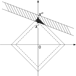
Figure 1: Illustration of Corollary 2. The shaded band area refers to the feasible domain of BPDN. The triangular area, the intersection of the feasible domain and the $\ell_{1}$ ball $\left\{\boldsymbol{x}:\left\|\boldsymbol{x}\right\|_{1}\leq\left\|\boldsymbol{x}^{o}\right\|_{1}\right\}$, is the set of all good recoveries.

An illustration of Corollary 2 is presented in Fig. 1, where the shaded band area refers to the feasible domain of BPDN in (4) and all points in the triangular area, the intersection of the feasible domain of BPDN and the $\ell_{1}$ ball $\left\{\boldsymbol{x}:\left\|\boldsymbol{x}\right\|_{1}\leq\left\|\boldsymbol{x}^{o}\right\|_{1}\right\}$, are good candidates for recovery of $\boldsymbol{x}^{o}$. The reason why one seeks for the optimal solution $\boldsymbol{x}^{*}$ is to guarantee that the inequality $\left\|\boldsymbol{x}\right\|_{1}\leq\left\|\boldsymbol{x}^{o}\right\|_{1}$ holds since $\left\|\boldsymbol{x}^{o}\right\|_{1}$ is generally unavailable a priori. Corollary 2 can explain why a satisfactory recovery can be obtained in practice using some algorithm that may not produce an optimal solution to BPDN, e.g., rONE-L1 [30]. Corollaries 1 and 2 are useful for checking the effectiveness of an algorithm in the case when the output cannot be guaranteed to be optimal. Namely, an algorithm is called effective in solving some $\ell_{1}$ minimization problem if it can produce a feasible solution with its $\ell_{1}$ norm no larger than that of the original signal. Similar ideas have been adopted in [32, 33].

III-F Application to DOA Estimation

DOA estimation is a classical problem in signal processing with many practical applications. Its research has recently been advanced owing to the development of CS based methods, e.g., $\ell_{1}$-SVD[34]. This subsection shows that the proposed SP-CS framework is applicable to the DOA estimation problem and hence has practical relevance. Consider $k$ narrowband far-field sources $s_{j}$, $j=1,\cdots,k$, impinging on an $m$-element uniform linear array (ULA) from directions $d_{j}$ with $d_{j}\in[0,\pi)$, $j=1,\cdots,k$. Denote $\boldsymbol{\theta}=\left[\cos\left(d_{1}\right),\dots,\cos\left(d_{k}\right)\right]^{T}\in(-1,1]^{k}$. For convenience, we consider the estimation of $\boldsymbol{\theta}$ rather than that of $\boldsymbol{d}$ hereafter. Moreover, we consider the noise free case for simplicity of exposition. Then the observation model is $\boldsymbol{y}=\boldsymbol{A}\left(\boldsymbol{\theta}\right)\boldsymbol{s}$ according to [35], where $\boldsymbol{y}\in\mathbb{C}^{m}$ denotes the vector of sensor measurements and $\boldsymbol{A}\left(\boldsymbol{\theta}\right)\in\mathbb{C}^{m\times k}$ denotes the sensing/measurement matrix with respect to $\boldsymbol{\theta}$ with $\boldsymbol{A}_{j}\left(\boldsymbol{\theta}\right)=\boldsymbol{a}\left(\theta_{j}\right)$ and $a_{l}\left(\theta_{j}\right)=\frac{1}{\sqrt{m}}\exp\left\{i\pi\left(l-\frac{m+1}{2}\right)\theta_{j}\right\}$, $j=1,\cdots,k$, $l=1,\cdots,m$, where $i=\sqrt{-1}$. The objective of DOA estimation is to estimate $\boldsymbol{\theta}$ given $\boldsymbol{y}$ and possibly $k$ as well. Since $k$ is typically small, CS based methods have been motivated in recent years. Let $\tilde{\boldsymbol{\theta}}=\left\{\frac{1}{n}-1,\frac{3}{n}-1,\cdots,1-\frac{1}{n}\right\}$ be a uniform sampling grid in $\boldsymbol{\theta}$ range $(-1,1]$ where $n$ denotes the grid number (without loss of generality, we assume that $n$ is an even number). In existing standard CS based methods $\tilde{\boldsymbol{\theta}}$ actually serves as the set of all candidate DOA estimates. As a result, their estimation accuracy is limited by the grid density since for some $\theta_{j}$, $j\in\left\{1,\cdots,k\right\}$, the best estimate of $\theta_{j}$ is its nearest grid point in $\tilde{\boldsymbol{\theta}}$. It can be easily shown that a lower bound for the mean squared estimation error of each $\theta_{j}$ is $\text{LB}=\frac{1}{3n^{2}}$ by assuming that $\theta_{j}$ is uniformly distributed in one or more grid intervals.

An off-grid model has been studied in [20, 12] that takes into account effects of the off-grid DOAs and introduces a structured matrix perturbation in the measurement matrix. For completeness, we re-derive it using Taylor expansion. Suppose $\theta_{j}\notin\tilde{\boldsymbol{\theta}}$ for some $j\in\left\{1,\cdots,k\right\}$ and that $\tilde{\theta}_{l_{j}}$, $l_{j}\in\left\{1,\cdots,n\right\}$, is the nearest grid point to $\theta_{j}$. By Taylor expansion we have

$$\boldsymbol{a}\left(\theta_{j}\right)=\boldsymbol{a}\left(\tilde{\theta}_{l_{j}}\right)+\boldsymbol{b}\left(\tilde{\theta}_{l_{j}}\right)\left(\theta_{j}-\tilde{\theta}_{l_{j}}\right)+\boldsymbol{R}_{j}$$ (19)

with $\boldsymbol{b}\left(\tilde{\theta}_{l_{j}}\right)=\boldsymbol{a}^{\prime}\left(\tilde{\theta}_{l_{j}}\right)$ and $\boldsymbol{R}_{j}$ being a remainder term with respect to $\theta_{j}$. Denote $\kappa=\frac{\pi}{2}\sqrt{\frac{m^{2}-1}{3}}$, $\boldsymbol{A}=\left[\boldsymbol{a}\left(\tilde{\theta}_{1}\right),\cdots,\boldsymbol{a}\left(\tilde{\theta}_{n}\right)\right]$, $\boldsymbol{B}={\kappa}^{-1}\left[\boldsymbol{b}\left(\tilde{\theta}_{1}\right),\cdots,\boldsymbol{b}\left(\tilde{\theta}_{n}\right)\right]$, and for $l=1,\cdots,n$,

$$\begin{array}[]{lll}\beta_{l}^{o}=\kappa\left(\theta_{j}-\tilde{\theta}_{l_{j}}\right),&x_{l}^{o}=s_{j},&\text{if }l=l_{j}\text{ for any }j\in\left\{1,\cdots,k\right\};\\ \beta_{l}^{o}=0,&x_{l}^{o}=0,&\text{otherwise},\end{array}$$

with $l_{j}\in\left\{1,\cdots,n\right\}$ and $\tilde{\theta}_{l_{j}}$ being the nearest grid to a source $\theta_{j}$, $j\in\left\{1,\cdots,k\right\}$. It is easy to show that $\left\|\boldsymbol{x}^{o}\right\|_{0}\leq k$, each column of $\boldsymbol{A}$ and $\boldsymbol{B}$ has unit norm, and $\boldsymbol{\beta}^{o}\in\left[-r,r\right]^{n}$ with $r=\frac{\kappa}{n}=\frac{\pi}{2n}\sqrt{\frac{m^{2}-1}{3}}$. In addition, we let $\boldsymbol{e}=\boldsymbol{R}\boldsymbol{s}$ with $\boldsymbol{R}=\left[\boldsymbol{R}_{1},\cdots,\boldsymbol{R}_{k}\right]$, and $\epsilon=\frac{\sqrt{k}\left\|\boldsymbol{s}\right\|_{2}\pi^{2}}{8n^{2}}\sqrt{\frac{3m^{4}-10m^{2}+7}{15}}$ such that $\left\|\boldsymbol{e}\right\|_{2}\leq\epsilon$ (the information of $k$ and $\left\|\boldsymbol{s}\right\|_{2}$ is used). The derivation for the setting of $\epsilon$ is provided in Appendix F. Then the DOA estimation model can be written into the form of our studied model in (9). The only differences are that $\boldsymbol{A}$, $\boldsymbol{B}$, $\boldsymbol{x}^{o}$ and $\boldsymbol{e}$ are in the complex domain rather than the real domain and that $\boldsymbol{e}$ denotes a modeling error term rather than the measurement noise. It is noted that the robust stability results in SP-CS apply straightforward to such complex signal case with few modifications. The objective turns to recovering $\boldsymbol{x}^{o}$ (its support actually) and $\boldsymbol{\beta}^{o}$. According to Theorem 4 $\boldsymbol{x}^{o}$ and $\boldsymbol{\beta}^{o}$ can be stably recovered if the D-RIP condition is satisfied. Denote $\widehat{\boldsymbol{x}}$ the recovered $\boldsymbol{x}^{o}$, $\widehat{\boldsymbol{\beta}}$ the recovered $\boldsymbol{\beta}^{o}$, and $\mathcal{I}$ the support of $\widehat{\boldsymbol{x}}$. Then we obtain the recovered $\boldsymbol{\theta}$: $\widehat{\boldsymbol{\theta}}=\tilde{\boldsymbol{\theta}}_{\mathcal{I}}+\kappa^{-1}\widehat{\boldsymbol{\beta}}_{\mathcal{I}}$ where $\boldsymbol{v}_{\mathcal{I}}$ keeps only entries of a vector $\boldsymbol{v}$ on the index set $\mathcal{I}$. The empirical results in Subsection V-B will illustrate the merits of applying the SP-CS framework to estimate DOAs.

Remark 5

• Within the scope of DOA estimation, this work is related to spectral CS introduced in [36]. To obtain an accurate solution, the authors of [36] adopt a very dense sampling grid (that is necessary for any standard CS based methods according to the mentioned lower bound for the mean squared estimation error) and then prohibit a solution whose support contains near-located indices (that correspond to highly coherent columns in the overcomplete dictionary). In this paper we show that accurate DOA estimation is possible by using a coarse grid and jointly estimating the off-grid distance (the distance from a true DOA to its nearest grid point).

• The off-grid DOA estimation problem has been studied in [20, 12]. The STLS solver in [20] obtains a maximum a posteriori solution if $\boldsymbol{\beta}^{o}$ is Gaussian distributed. But such a condition does not hold in the off-grid DOA estimation problem. The SBI solver in [12] proposed by the authors is based on the same model as in (9) and within the framework of Bayesian CS [37].

• The proposed P-BPDN can be extended to the multiple measurement vectors case like $\ell_{1}$-SVD to deal with DOA estimation with multiple snapshots.

IV Algorithms for P-BPDN

IV-A Special Case: Positive Signals

This subsection studies a special case where the original signal $\boldsymbol{x}^{o}$ is positive-valued (except zero entries). Such a case has been studied in standard CS [38, 39]. By incorporating the positiveness of $\boldsymbol{x}^{o}$, P-BPDN is modified into the positive P-BPDN (PP-BPDN) problem

$$\min_{\boldsymbol{x},\boldsymbol{\beta}}\boldsymbol{1}^{T}\boldsymbol{x},\text{ subject to }\left\{\begin{array}[]{l}\left\|\boldsymbol{y}-\left(\boldsymbol{A}+\boldsymbol{B}\boldsymbol{\Delta}\right)\boldsymbol{x}\right\|_{2}\leq\epsilon,\\ \boldsymbol{x}\succcurlyeq\boldsymbol{0},\\ r\boldsymbol{1}\succcurlyeq\boldsymbol{\beta}\succcurlyeq-r\boldsymbol{1},\end{array}\right.$$

where $\succcurlyeq$ is $\geq$ with an elementwise operation and $\boldsymbol{0}$, $\boldsymbol{1}$ are column vectors composed of $0$, $1$ respectively with proper dimensions. It is noted that the robustly stable signal recovery results in the present paper apply directly to the solution to PP-BPDN in such case. This subsection shows that the nonconvex PP-BPDN problem can be transformed into a convex one and hence its optimal solution can be efficiently obtained. Denote $\boldsymbol{p}=\boldsymbol{\beta}\odot\boldsymbol{x}$. A new, convex problem $\left(P_{1}\right)$ is introduced as follows.

$$\left(P_{1}\right)\quad\min_{\boldsymbol{x},\boldsymbol{p}}\boldsymbol{1}^{T}\boldsymbol{x},\text{ subject to }\left\{\begin{array}[]{l}\left\|\boldsymbol{y}-\boldsymbol{\Psi}\begin{bmatrix}\boldsymbol{x}\\ \boldsymbol{p}\end{bmatrix}\right\|_{2}\leq\epsilon,\\ \boldsymbol{x}\succcurlyeq\boldsymbol{0},\\ r\boldsymbol{x}\succcurlyeq\boldsymbol{p}\succcurlyeq-r\boldsymbol{x}.\end{array}\right.$$

Theorem 6

Problems PP-BPDN and $\left(P_{1}\right)$ are equivalent in the sense that, if $\left(\boldsymbol{x}^{*},\boldsymbol{\beta}^{*}\right)$ is an optimal solution to PP-BPDN, then there exists $\boldsymbol{p}^{*}=\boldsymbol{\beta}^{*}\odot\boldsymbol{x}^{*}$ such that $\left(\boldsymbol{x}^{*},\boldsymbol{p}^{*}\right)$ is an optimal solution to $\left(P_{1}\right)$, and that, if $\left(\boldsymbol{x}^{*},\boldsymbol{p}^{*}\right)$ is an optimal solution to $\left(P_{1}\right)$, then there exists $\boldsymbol{\beta}^{*}$ with $\beta^{*}_{j}=\left\{\begin{array}[]{l}p_{j}^{*}/x_{j}^{*},\\ 0,\end{array}\begin{array}[]{l}\text{ if }x_{j}^{*}>0;\\ \text{ otherwise}\end{array}\right.$ such that $\left(\boldsymbol{x}^{*},\boldsymbol{\beta}^{*}\right)$ is an optimal solution to PP-BPDN.

Proof:

We only prove the first part of Theorem 6 using contradiction. The second part follows similarly. Suppose that $\left(\boldsymbol{x}^{*},\boldsymbol{p}^{*}\right)$ with $\boldsymbol{p}^{*}=\boldsymbol{\beta}^{*}\odot\boldsymbol{x}^{*}$ is not an optimal solution to $\left(P_{1}\right)$. Then there exists $\left(\boldsymbol{x}^{\prime},\boldsymbol{p}^{\prime}\right)$ in the feasible domain of $\left(P_{1}\right)$ such that $\left\|\boldsymbol{x}^{\prime}\right\|_{1}<\left\|\boldsymbol{x}^{*}\right\|_{1}$. Define $\boldsymbol{\beta}^{\prime}$ as $\beta^{\prime}_{j}=\left\{\begin{array}[]{l}p^{\prime}_{j}/x^{\prime}_{j},\\ 0,\end{array}\begin{array}[]{l}\text{ if }x^{\prime}_{j}>0;\\ \text{ otherwise}\end{array}\right.$. It is easy to show that $\left(\boldsymbol{x}^{\prime},\boldsymbol{\beta}^{\prime}\right)$ is a feasible solution to PP-BPDN. By $\left\|\boldsymbol{x}^{\prime}\right\|_{1}<\left\|\boldsymbol{x}^{*}\right\|_{1}$ we conclude that $\left(\boldsymbol{x}^{*},\boldsymbol{\beta}^{*}\right)$ is not an optimal solution to PP-BPDN, which leads to contradiction.  

Theorem 6 states that an optimal solution to PP-BPDN can be efficiently obtained by solving the convex problem $\left(P_{1}\right)$.

IV-B AA-P-BPDN: Alternating Algorithm for P-BPDN

For general signals, P-BPDN in (11) is nonconvex. A simple method is to solve a series of BPDN problems with

$$\boldsymbol{x}^{\left(j+1\right)} = \arg\min_{\boldsymbol{x}}\left\|\boldsymbol{x}\right\|_{1},\text{ subject to }$$ (20)

$$\left\|\boldsymbol{y}-\left(\boldsymbol{A}+\boldsymbol{B}\boldsymbol{\Delta}^{\left(j\right)}\right)\boldsymbol{x}\right\|_{2}\leq\epsilon,$$

$$\boldsymbol{\beta}^{\left(j+1\right)} = \arg\min_{\boldsymbol{\beta}\in\left[-r,r\right]^{n}}\left\|\boldsymbol{y}-\left(\boldsymbol{A}+\boldsymbol{B}\boldsymbol{\Delta}\right)\boldsymbol{x}^{\left(j+1\right)}\right\|_{2}$$ (21)

starting from $\boldsymbol{\beta}^{\left(0\right)}=\boldsymbol{0}$, where the superscript ^(j) indicates the $j$th iteration and $\boldsymbol{\Delta}^{\left(j\right)}=\text{diag}\left(\boldsymbol{\beta}^{\left(j\right)}\right)$. Denote AA-P-BPDN the alternating algorithm defined by (20) and (21). To analyze AA-P-BPDN, we first present the following two lemmas.

Lemma 1

For a matrix sequence $\left\{\boldsymbol{\Phi}^{\left(j\right)}\right\}_{j=1}^{\infty}$ composed of fat matrices, let $\mathcal{D}^{j}=\left\{\boldsymbol{v}:\left\|\boldsymbol{y}-\boldsymbol{\Phi}^{\left(j\right)}\boldsymbol{v}\right\|_{2}\leq\epsilon\right\}$, $j=1,2,\cdots$, and $\mathcal{D}^{*}=\left\{\boldsymbol{v}:\left\|\boldsymbol{y}-\boldsymbol{\Phi}^{*}\boldsymbol{v}\right\|_{2}\leq\epsilon\right\}$ with $\epsilon>0$. If $\boldsymbol{\Phi}^{\left(j\right)}\rightarrow\boldsymbol{\Phi}^{*}$, as $j\rightarrow+\infty$, then for any $\boldsymbol{v}\in\mathcal{D}^{*}$ there exists a sequence $\left\{\boldsymbol{v}^{\left(j\right)}\right\}_{j=1}^{\infty}$ with $\boldsymbol{v}^{\left(j\right)}\in\mathcal{D}^{\left(j\right)}$, $j=1,2,\cdots$, such that $\boldsymbol{v}^{\left(j\right)}\rightarrow\boldsymbol{v}$, as $j\rightarrow+\infty$.

Lemma 1 studies the variation of feasible domains $\mathcal{D}^{j}$, $j=1,2,\cdots$, of a series of BPDN problems whose sensing matrices $\boldsymbol{\Phi}^{\left(j\right)}$, $j=1,2,\cdots$, converge to $\boldsymbol{\Phi}^{*}$. It states that the sequence of the feasible domains also converges to $\mathcal{D}^{*}$ in the sense that for any point in $\mathcal{D}^{*}$, there exists a sequence of points, each of which belongs to one $\mathcal{D}^{j}$, that converges to the point. To prove Lemma 1, we first show that it holds for any interior point of $\mathcal{D}^{*}$ by constructing such a sequence. Then we show that it also holds for a boundary point of $\mathcal{D}^{*}$ by that for any boundary point there exists a sequence of interior points of $\mathcal{D}^{*}$ that converges to it. The detailed proof is given in Appendix C.

Lemma 2

An optimal solution $\boldsymbol{x}^{*}$ to the BPDN problem in (4) satisfies that $\boldsymbol{x}^{*}=\boldsymbol{0}$, if $\left\|\boldsymbol{y}\right\|_{2}\leq\epsilon$, or $\left\|\boldsymbol{y}-\boldsymbol{\Phi}\boldsymbol{x}^{*}\right\|_{2}=\epsilon$, otherwise.

Proof:

It is trivial for the case where $\left\|\boldsymbol{y}\right\|_{2}\leq\epsilon$. Consider the other case where $\left\|\boldsymbol{y}\right\|_{2}>\epsilon$. Note first that $\boldsymbol{x}^{*}\neq\boldsymbol{0}$. We use contradiction to show that the equality $\left\|\boldsymbol{y}-\boldsymbol{\Phi}\boldsymbol{x}^{*}\right\|_{2}=\epsilon$ holds. Suppose that $\left\|\boldsymbol{y}-\boldsymbol{\Phi}\boldsymbol{x}^{*}\right\|_{2}<\epsilon$. Introduce $f\left(\theta\right)=\left\|\boldsymbol{y}-\theta\boldsymbol{\Phi}\boldsymbol{x}^{*}\right\|_{2}$. Then $f(0)>\epsilon$, and $f(1)<\epsilon$. There exists $\theta_{0}$, $0<\theta_{0}<1$, such that $f\left(\theta_{0}\right)=\epsilon$ since $f\left(\theta\right)$ is continuous on the interval $\left[0,1\right]$. Hence, $\boldsymbol{x}^{\prime}=\theta_{0}\boldsymbol{x}^{*}$ is a feasible solution to BPDN in (4). We conclude that $\boldsymbol{x}^{*}$ is not optimal by $\left\|\boldsymbol{x}^{\prime}\right\|_{1}=\theta_{0}\left\|\boldsymbol{x}^{*}\right\|_{1}<\left\|\boldsymbol{x}^{*}\right\|_{1}$, which leads to contradiction.  

Lemma 2 studies the location of an optimal solution to the BPDN problem. It states that the optimal solution locates at the origin if the origin is a feasible solution, or at the boundary of the feasible domain otherwise. This can be easily observed from Fig. 1. Based on Lemmas 1 and 2, we have the following results for AA-P-BPDN.

Theorem 7

Any accumulation point $\left(\boldsymbol{x}^{*},\boldsymbol{\beta}^{*}\right)$ of the sequence $\left\{\left(\boldsymbol{x}^{\left(j\right)},\boldsymbol{\beta}^{\left(j\right)}\right)\right\}_{j=1}^{\infty}$ is a stationary point of AA-P-BPDN in the sense that

$$\boldsymbol{x}^{*} = \arg\min_{\boldsymbol{x}}\left\|\boldsymbol{x}\right\|_{1},\text{ subject to }$$ (22)

$$\left\|\boldsymbol{y}-\left(\boldsymbol{A}+\boldsymbol{B}\boldsymbol{\Delta}^{*}\right)\boldsymbol{x}\right\|_{2}\leq\epsilon,$$

$$\boldsymbol{\beta}^{*} = \arg\min_{\boldsymbol{\beta}\in\left[-r,r\right]^{n}}\left\|\boldsymbol{y}-\left(\boldsymbol{A}+\boldsymbol{B}\boldsymbol{\Delta}\right)\boldsymbol{x}^{*}\right\|_{2}$$ (23)

with $\boldsymbol{\Delta}^{*}=\text{diag}\left(\boldsymbol{\beta}^{*}\right)$.

Theorem 8

An optimal solution $\left(\boldsymbol{x}^{*},\boldsymbol{\beta}^{*}\right)$ to P-BPDN in (11) is a stationary point of AA-P-BPDN.

Theorem 7 studies the property of the solution $\left(\boldsymbol{x}^{\left(j\right)},\boldsymbol{\beta}^{\left(j\right)}\right)$ produced by AA-P-BPDN. It shows that $\left(\boldsymbol{x}^{\left(j\right)},\boldsymbol{\beta}^{\left(j\right)}\right)$ is arbitrarily close to a stationary point of AA-P-BPDN as the iteration index $j$ is large enough. Hence, the output of AA-P-BPDN can be considered as a stationary point provided that an appropriate termination criterion is set. Theorem 8 tells that an optimal solution to P-BPDN is a stationary point of AA-P-BPDN. So, it is possible for AA-P-BPDN to produce an optimal solution to P-BPDN. The proofs of Theorems 7 and 8 are provided in Appendix D and Appendix E respectively.

Remark 6

During the revision of this paper, we have noted the following formulation of P-BPDN that possibly can provide an efficient approach to an optimal solution to P-BPDN. Let $\boldsymbol{x}=\boldsymbol{x}_{+}-\boldsymbol{x}_{-}$ where $\boldsymbol{x}_{+}\succcurlyeq\boldsymbol{0}$, $\boldsymbol{x}_{-}\succcurlyeq\boldsymbol{0}$ and $\boldsymbol{x}_{+}\odot\boldsymbol{x}_{-}=\boldsymbol{0}$. Then we have $\left|\boldsymbol{x}\right|=\boldsymbol{x}_{+}+\boldsymbol{x}_{-}$ where $\left|\cdot\right|$ applies elementwise. Denote $\boldsymbol{p}=\boldsymbol{\beta}\odot\boldsymbol{x}$. A convex problem can be cast as follows:

$$\begin{split}&\min_{\boldsymbol{x}_{+},\boldsymbol{x}_{-},\boldsymbol{p}}\boldsymbol{1}^{T}\left(\boldsymbol{x}_{+}+\boldsymbol{x}_{-}\right),\\ &\text{ subject to }\left\{\begin{array}[]{l}\left\|\boldsymbol{y}-\begin{bmatrix}\boldsymbol{A}&-\boldsymbol{A}&\boldsymbol{B}\end{bmatrix}\begin{bmatrix}\boldsymbol{x}_{+}\\ \boldsymbol{x}_{-}\\ \boldsymbol{p}\end{bmatrix}\right\|_{2}\leq\epsilon,\\ \boldsymbol{x}_{+}\succcurlyeq\boldsymbol{0},\\ \boldsymbol{x}_{-}\succcurlyeq\boldsymbol{0},\\ r\left(\boldsymbol{x}_{+}+\boldsymbol{x}_{-}\right)\succcurlyeq\boldsymbol{p}\succcurlyeq-r\left(\boldsymbol{x}_{+}+\boldsymbol{x}_{-}\right).\end{array}\right.\end{split}$$ (24)

The above convex problem can be considered as a convex relaxation of P-BPDN since it can be shown (like that in Theorem 6) that an optimal solution to P-BPDN can be obtained based on an optimal solution to the problem in (24) incorporated with an additional nonconvex constraint $\boldsymbol{x}_{+}\odot\boldsymbol{x}_{-}=\boldsymbol{0}$. An interesting phenomenon has been observed through numerical simulations that an optimal solution to the problem in (24) still satisfies the constraint $\boldsymbol{x}_{+}\odot\boldsymbol{x}_{-}=\boldsymbol{0}$. Based on such an observation, an efficient approach to P-BPDN is to firstly solve (24), and then check whether its solution, denoted by $\left(\boldsymbol{x}_{+}^{*},\boldsymbol{x}_{-}^{*},\boldsymbol{p}^{*}\right)$, satisfies $\boldsymbol{x}_{+}\odot\boldsymbol{x}_{-}=\boldsymbol{0}$. If it does, then $\left(\boldsymbol{x}^{*},\boldsymbol{\beta}^{*}\right)$ is an optimal solution to P-BPDN where $\boldsymbol{x}^{*}=\boldsymbol{x}_{+}^{*}-\boldsymbol{x}_{-}^{*}$ and $\beta^{*}_{j}=\left\{\begin{array}[]{l}p_{j}^{*}/x_{j}^{*},\\ 0,\end{array}\begin{array}[]{l}\text{ if }x_{j}^{*}\neq 0;\\ \text{ otherwise.}\end{array}\right.$ Otherwise, we may turn to AA-P-BPDN again. But we note that it is still an open problem whether an optimal solution to (24) always satisfies the constraint $\boldsymbol{x}_{+}\odot\boldsymbol{x}_{-}=\boldsymbol{0}$. In addition, the convex relaxation in (24) does not apply to the complex signal case as in DOA estimation studied in Subsection III-F.

IV-C Effectiveness of AA-P-BPDN

As reported in the last subsection, it is possible for AA-P-BPDN to produce an optimal solution to P-BPDN. But it is not easy to check the optimality of the output of AA-P-BPDN because of the nonconvexity of P-BPDN. Instead, we study the effectiveness of AA-P-BPDN in solving P-BPDN in this subsection with the concept of effectiveness as defined in Subsection III-E. By Corollary 1, a good signal recovery $\widehat{\boldsymbol{x}}$ of $\boldsymbol{x}^{o}$ is not necessarily an optimal solution. It requires only that $\left(\widehat{\boldsymbol{x}},\widehat{\boldsymbol{\beta}}\right)$, where $\widehat{\boldsymbol{\beta}}$ denotes the recovery of $\boldsymbol{\beta}^{o}$, be a feasible solution to P-BPDN and that $\left\|\widehat{\boldsymbol{x}}\right\|_{1}\leq\left\|\boldsymbol{x}^{o}\right\|_{1}$ holds. As shown in the proof of Theorem 7 in Appendix D, that $\left(\boldsymbol{x}^{\left(j\right)},\boldsymbol{\beta}^{\left(j\right)}\right)$ for any $j\geq 1$ is a feasible solution to P-BPDN and that the sequence $\left\{\left\|\boldsymbol{x}^{\left(j\right)}\right\|_{1}\right\}_{j=1}^{\infty}$ is monotone decreasing and converges. So, the effectiveness of AA-P-BPDN in solving P-BPDN can be assessed via numerical simulations by checking whether $\left\|\boldsymbol{x}^{AA}\right\|_{1}\leq\left\|\boldsymbol{x}^{o}\right\|_{1}$ holds with $\boldsymbol{x}^{AA}$ denoting the output of AA-P-BPDN. The effectiveness of AA-P-BPDN is verified in Subsection V-A via numerical simulations, where we observe that the inequality $\left\|\boldsymbol{x}^{AA}\right\|_{1}\leq\left\|\boldsymbol{x}^{o}\right\|_{1}$ holds in all experiments (over $3700$ trials).

V Numerical Simulations

V-A Verification of the Robust Stability

This subsection demonstrates the robustly stable signal recovery results of SP-CS in the present paper, as well as the effectiveness of AA-P-BPDN in solving P-BPDN in (11), via numerical simulations. AA-P-BPDN is implemented in Matlab with problems in (20) and (21) being solved using CVX [40]. AA-P-BPDN is terminated as $\frac{\left|\left\|\boldsymbol{x}^{\left(j\right)}\right\|_{1}-\left\|\boldsymbol{x}^{\left(j-1\right)}\right\|_{1}\right|}{\left\|\boldsymbol{x}^{\left(j-1\right)}\right\|_{1}}\leq 1\times 10^{-6}$ or the maximum number of iterations, set to $200$, is reached. PP-BPDN is also implemented in Matlab and solved by CVX.

We first consider general signals. The sparse signal case is mainly studied. The variation of the signal recovery error is studied with respect to the noise level, perturbation level and number of measurements respectively. Besides AA-P-BPDN for P-BPDN in SP-CS, performances of three other approaches are also studied. The first one assumes that the perturbation is known a priori and recovers the original signal $\boldsymbol{x}^{o}$ by solving, namely, the oracle (O-) BPDN problem

$$\min_{\boldsymbol{x}}\left\|\boldsymbol{x}\right\|_{1},\text{ subject to }\left\|\boldsymbol{y}-\left(\boldsymbol{A}+\boldsymbol{B}\boldsymbol{\Delta}^{o}\right)\boldsymbol{x}\right\|_{2}\leq\epsilon.$$

The O-BPDN approach produces the best recovery result of SP-CS within the scope of $\ell_{1}$ minimization of CS since it exploits the exact perturbation (oracle information). The second one corresponds to the robust signal recovery of perturbed CS as described in Subsection II-C and solves N-BPDN in (7) where $\epsilon_{\boldsymbol{E},\boldsymbol{x}^{o}}=\left\|\boldsymbol{B}\boldsymbol{\Delta}^{o}\boldsymbol{x}^{o}\right\|_{2}$ is used though it is not available in practice. The last one refers to the other approach to SP-CS that seeks for the signal recovery by solving TPS-BPDN in (16) as discussed in Subsection III-E.

The first experiment studies the signal recovery error with respect to the noise level. We set the signal length $n=200$, sample size $m=80$, sparsity level $k=10$ and perturbation parameter $r=0.1$. The noise level $\epsilon$ varies from $0.05$ to $2$ with interval $0.05$. For each combination of $\left(n,m,k,r,\epsilon\right)$, the signal recovery error, as well as $\boldsymbol{\beta}^{o}$ recovery error (on the support of $\boldsymbol{x}^{o}$), is averaged over $R=50$ trials. In each trial, matrices $\boldsymbol{A}$ and $\boldsymbol{B}$ are generated from Gaussian distribution and each column of them has zero mean and unit norm after proper scaling. The sparse signal $\boldsymbol{x}^{o}$ is composed of unit spikes with random signs and locations. Entries of $\boldsymbol{\beta}^{o}$ are uniformly distributed in $\left[-r,r\right]$. The noise $\boldsymbol{e}$ is zero mean Gaussian distributed and then scaled such that $\left\|\boldsymbol{e}\right\|_{2}=\epsilon$. Using the same data, the four approaches, including O-BPDN, N-BPDN, TPS-BPDN and AA-P-BPDN for P-BPDN, are used to recover $\boldsymbol{x}^{o}$ respectively in each trial. The simulation results are shown in Fig. 2. It can be seen that both signal and $\boldsymbol{\beta}^{o}$ recovery errors of AA-P-BPDN for P-BPDN in SP-CS are proportional to the noise, which is consistent with our robustly stable signal recovery result in the present paper. The error of N-BPDN grows linearly with the noise but a large error still exhibits in the noise free case. Except the ideal case of O-BPDN, our proposed P-BPDN has the smallest error.

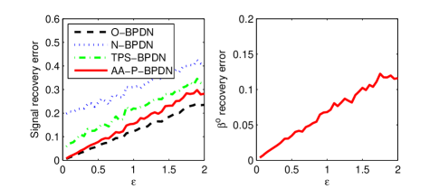
Figure 2: Signal and perturbation recovery errors with respect to the noise level $\epsilon$ with parameter settings $\left(n,m,k,r\right)=\left(200,80,10,0.1\right)$. Both signal and $\boldsymbol{\beta}^{o}$ recovery errors of AA-P-BPDN for P-BPDN in SP-CS are proportional to $\epsilon$.

The second experiment studies the effect of the structured perturbation. Experiment settings are the same as those in the first experiment except that we set $\left(n,m,k,\epsilon\right)=\left(200,80,10,0.5\right)$ and vary $r\in\left\{0.05,0.1,\cdots,1\right\}$. Fig. 3 presents our simulation results. A nearly constant error is obtained using O-BPDN in standard CS since the perturbation is assumed to be known in O-BPDN. The error of AA-P-BPDN for P-BPDN in SP-CS slowly increases with the perturbation level and is quite close to that of O-BPDN for a moderate perturbation. Such a behavior is consistent with our analysis. Besides, it can be observed that the error of N-BPDN grows linearly with the perturbation level. Again, our proposed P-BPDN has the smallest error except O-BPDN.

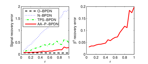
Figure 3: Signal and perturbation recovery errors with respect to the perturbation level in terms of $r$ with parameter settings $\left(n,m,k,\epsilon\right)=\left(200,80,10,0.5\right)$. The error of AA-P-BPDN for P-BPDN in SP-CS slowly increases with the perturbation level and is quite close to that of the ideal case of O-BPDN for a moderate perturbation.

The third experiment studies the variation of the recovery error with the number of measurements. We set $\left(n,k,r,\epsilon\right)=\left(200,10,0.1,0.2\right)$ and vary $m\in\left\{30,35,\cdots,100\right\}$. Simulation results are presented in Fig. 4. Signal recovery errors of all four approaches decrease as the number of measurements increases. Again, it is observed that O-BPDN of the ideal case achieves the best result followed by our proposed P-BPDN. For example, to obtain the signal recovery error of $0.05$, about $55$ measurements are needed for O-BPDN while the numbers are, respectively, $65$ for AA-P-BPDN and $95$ for TPS-BPDN. It is impossible for N-BPDN to achieve such a small error in our observation because of the existence of the perturbation.

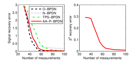
Figure 4: Signal and perturbation recovery errors with respect to the number of measurements with parameter settings $\left(n,k,r,\epsilon\right)=\left(200,10,0.1,0.2\right)$. AA-P-BPDN for P-BPDN in SP-CS has the best performance except the ideal case of O-BPDN.

We next consider a compressible signal that is generated by taking a fixed sequence $\left\{2.8843\cdot j^{-1.5}\right\}_{j=1}^{n}$ with $n=200$, randomly permuting it, and multiplying by a random sign sequence (the coefficient $2.8843$ is chosen such that the compressible signal has the same $\ell_{2}$ norm as the sparse signals in the previous experiments). It is sought to be recovered from $m=70$ noisy measurements with $\epsilon=0.2$ and $r=0.1$. Give experiment results in one instance as an example. The signal recovery error of AA-P-BPDN for P-BPDN in SP-CS is about $0.239$, while errors of O-BPDN, N-BPDN and TPS-BPDN are about $0.234$, $0.361$ and $0.314$ respectively.

For the special positive signal case, an optimal solution to PP-BPDN can be efficiently obtained. An experiment result is shown in Fig. 5, where a sparse signal of length $n=200$, composed of $k=10$ positive unit spikes, is exactly recovered from $m=50$ noise free measurements with $r=0.1$ by solving $\left(P_{1}\right)$.

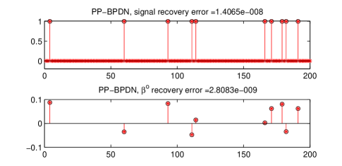
Figure 5: Exact recovery of a positive sparse signal from noise-free measurements with $\left(m,n,k,r,\epsilon\right)=\left(200,50,10,0.1,0\right)$. PP-BPDN is solved by solving $\left(P_{1}\right)$. $\boldsymbol{\beta}^{o}$ and its recovery are shown only on the support of $\boldsymbol{x}^{o}$. Black circles: original signal and $\boldsymbol{\beta}^{o}$; red stars: recoveries.

V-B Empirical Results of DOA Estimation

This subsection studies the empirical performance of the application of the studied SP-CS framework in DOA estimation. We consider the case of $n=90$ and $k=2$. Numerical calculations show that the D-RIP condition $\bar{\delta}_{4k}\left(\boldsymbol{\Psi}\right)<\left(\sqrt{2\left(1+r^{2}\right)}+1\right)^{-1}$ in Theorem 4 is satisfied if $m\geq 145$. Though it ceases to be a “compressed” sensing problem in the case $m\geq n$, it still makes sense in SP-CS since there are $2n$ variables to be estimated and hence the P-BPDN problem is still underdetermined as $m<2n$. As noted in Subsection III-C, the D-RIP condition can be possibly relaxed using recent techniques in standard CS, which may reduce the required $m$ value. In addition, a RIP condition is a sufficient condition for guaranteed signal recovery accuracy while its conservativeness in standard CS has been studied in [41]. We next choose a much smaller $m=30$ ($r\approx 0.302$ in such a case) and show the empirical performance of the proposed SP-CS framework on such off-grid DOA estimation.

The experimental setup is as follows. In each trial, the complex source signal $\boldsymbol{s}$ is generated with both entries having unit amplitude and random phases. $\theta_{1}$ and $\theta_{2}$ are generated uniformly from intervals $\left[\frac{2}{n},\frac{4}{n}\right]$ and $\left[\frac{12}{n},\frac{14}{n}\right]$ respectively ($5.1^{\circ}\sim 7.7^{\circ}$ apart in the DOA domain). P-BPDN is solved using AA-P-BPDN whose settings are the same as those in Subsection V-A. Our experimental results of the estimation error $\widehat{\boldsymbol{\theta}}-\boldsymbol{\theta}$ for both sources are presented in Fig. 6 where 1000 trials are used. It can be seen that P-BPDN performs well on the off-grid DOA estimation. All estimation errors lie in the interval $\left[-\frac{1}{n},\frac{1}{n}\right]$ with most very close to zero. To achieve a possibly comparable mean squared estimation error, a grid of length at least $n=360$ has to be used in standard CS based methods according to the lower bound mentioned in Subsection III-F. An example of performance of SP-CS and standard CS on DOA estimation is shown in Fig. 7, where the two approaches share the same data set and $n=360$ is set in standard CS. From the upper two sub-figures, it can be seen that SP-CS performs well on both source signal and $\boldsymbol{\beta}^{o}$ recoveries. From the lower left one, however, it can be seen that two nonzero entries are presented in the recovered signal around the location of each source when using standard CS. Such a phenomenon is much clearer in the last sub-figure, where it can be observed that a single peak exhibits at a place very close to the true location of source 1 using the proposed SP-CS framework while two peaks occurs at places further away from the true source in standard CS.

Figure 6: Histogram of $\boldsymbol{\theta}$ estimation error for both sources using P-BPDN for SP-CS. Statistics including mean, variance and mean squared error (MSE) are shown.

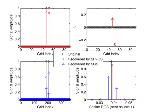
Figure 7: Performance comparison of SP-CS and standard CS (SCS) on DOA estimation. Upper left: signal recovery in SP-CS; upper right: $\boldsymbol{\beta}^{o}$ recovery in SP-CS (shown only on the signal support); lower left: signal recovery in standard CS; lower right: signal amplitude versus $\theta$ (near the location of source 1) in SP-CS and standard CS.

VI Conclusion

This paper studied the CS problem in the presence of measurement noise and a structured matrix perturbation. A concept named as robust stability for signal recovery was introduced. It was shown that the robust stability can be achieved for a sparse signal by solving an $\ell_{1}$ minimization problem P-BPDN under mild conditions. In the presence of measurement noise, the recovery error is at most proportional to the noise level and the recovery is exact in the special noise free case. A general result for compressible signals was also reported. An alternating algorithm named as AA-P-BPDN was proposed to solve the nonconvex P-BPDN problem, and numerical simulations were carried out, verifying our theoretical analysis. A practical application in DOA estimation was studied and satisfactory estimation results were obtained.

The simulation results of DOA estimation suggest that the RIP condition for the robust stability is quite conservative in practice. One future work is to relax such a condition. In our problem formulation, the signal $\boldsymbol{x}^{o}$ and $\boldsymbol{\beta}^{o}$ that determines the matrix perturbation are jointly sparse. While this paper focuses on extracting the information that $\boldsymbol{x}^{o}$ is sparse and that each entry of $\boldsymbol{\beta}^{o}$ lies in a bounded interval, such joint sparsity is not exploited. Inspired by the recent works on block and structured sparsity, e.g., [42, 43], one future direction is to take into account the joint sparsity information in the signal recovery process to obtain possibly improved recovery performance. Our studied perturbed CS problem is related to the area of dictionary learning for sparse representation [44], where there is typically no a priori known structure in the overcomplete dictionary and a large number of observation vectors are important to make the learning process succeed. The studied problem in this paper can be considered as a dictionary learning problem but with a known structure in the dictionary, which leads to some similarity between our optimization approach and algorithms for dictionary learning, e.g., $K$-SVD [44] and MOD [45]. Due to the known structure, it has been shown in this paper that a single observation vector is enough to learn the dictionary with guaranteed performance. Further relations deserve future studies.

Appendix A
Proof of Theorem 3

Denote $\boldsymbol{z}=\begin{bmatrix}\boldsymbol{x}\\ \boldsymbol{\beta}\odot\boldsymbol{x}\end{bmatrix}$ and similarly define $\boldsymbol{z}^{o}$ and $\boldsymbol{z}^{*}$. Then the problem in (10) can be rewritten into

$$\min_{\boldsymbol{x}\in\mathbb{R}^{n},\boldsymbol{\beta}\in\left[-r,r\right]^{n}}\left\|\boldsymbol{x}\right\|_{0},\text{ subject to }\boldsymbol{y}=\boldsymbol{\Psi}\boldsymbol{z}.$$ (25)

Let $\bar{\delta}_{k}=\bar{\delta}_{k}\left(\boldsymbol{\Psi}\right)$ hereafter for brevity.

First note that $\boldsymbol{x}^{o}$ is $k$-sparse and $\boldsymbol{z}^{o}$ is $2k$-D-sparse. Since $\left(\boldsymbol{x}^{*},\boldsymbol{\beta}^{*}\right)$ is a solution to the problem in (25), we have $\left\|\boldsymbol{x}^{*}\right\|_{0}\leq\left\|\boldsymbol{x}^{o}\right\|_{0}\leq k$ and, hence, $\boldsymbol{z}^{*}$ is $2k$-D-sparse. By $\boldsymbol{y}=\boldsymbol{\Psi}\boldsymbol{z}^{o}=\boldsymbol{\Psi}\boldsymbol{z}^{*}$ we obtain $\boldsymbol{\Psi}\left(\boldsymbol{z}^{o}-\boldsymbol{z}^{*}\right)=\boldsymbol{0}$ and thus $\boldsymbol{z}^{o}-\boldsymbol{z}^{*}=\boldsymbol{0}$ by $\bar{\delta}_{4k}<1$ and the fact that $\boldsymbol{z}^{o}-\boldsymbol{z}^{*}$ is $4k$-D-sparse. We complete the proof by observing that $\boldsymbol{z}^{o}-\boldsymbol{z}^{*}=\begin{bmatrix}\boldsymbol{x}^{o}-\boldsymbol{x}^{*}\\ \boldsymbol{\beta}^{o}\odot\boldsymbol{x}^{o}-\boldsymbol{\beta}^{*}\odot\boldsymbol{x}^{*}\end{bmatrix}=\boldsymbol{0}$.

Appendix B
Proofs of Theorems 4 and 5

We only present the proof of Theorem 5 since Theorem 4 is a special case of Theorem 5. We first show the following lemma.

Lemma 3

We have

$$\left|\left\langle\boldsymbol{\Psi}\boldsymbol{v},\boldsymbol{\Psi}\boldsymbol{v}^{\prime}\right\rangle\right|\leq\bar{\delta}_{2(k+k^{\prime})}\left\|\boldsymbol{v}\right\|_{2}\left\|\boldsymbol{v}^{\prime}\right\|_{2}$$

for all $2k$-D-sparse $\boldsymbol{v}$ and $2k^{\prime}$-D-sparse $\boldsymbol{v}^{\prime}$ supported on disjoint subsets.

Proof:

Without loss of generality, assume that $\boldsymbol{v}$ and $\boldsymbol{v}^{\prime}$ are unit vectors with disjoint supports as above. Then by the definition of D-RIP and $\left\|\boldsymbol{v}\pm\boldsymbol{v}^{\prime}\right\|_{2}^{2}=\left\|\boldsymbol{v}\right\|_{2}^{2}+\left\|\boldsymbol{v}^{\prime}\right\|_{2}^{2}=2$ we have

$$2\left(1-\bar{\delta}_{2\left(k+k^{\prime}\right)}\right)\leq\left\|\boldsymbol{\Psi}\boldsymbol{v}\pm\boldsymbol{\Psi}\boldsymbol{v}^{\prime}\right\|_{2}^{2}\leq 2\left(1+\bar{\delta}_{2\left(k+k^{\prime}\right)}\right).$$

And thus

$$\left|\left\langle\boldsymbol{\Psi}\boldsymbol{v},\boldsymbol{\Psi}\boldsymbol{v}^{\prime}\right\rangle\right|\leq\frac{1}{4}\left|\left\|\boldsymbol{\Psi}\boldsymbol{v}+\boldsymbol{\Psi}\boldsymbol{v}^{\prime}\right\|_{2}^{2}-\left\|\boldsymbol{\Psi}\boldsymbol{v}-\boldsymbol{\Psi}\boldsymbol{v}^{\prime}\right\|_{2}^{2}\right|\leq\bar{\delta}_{2\left(k+k^{\prime}\right)},$$

which completes the proof.  

Using the notations $\boldsymbol{z}$, $\boldsymbol{z}^{o}$, $\boldsymbol{z}^{*}$ and $\bar{\delta}_{k}$ in Appendix A, P-BPDN in (11) can be rewritten into

$$\min_{\boldsymbol{x}\in\mathbb{R}^{n},\boldsymbol{\beta}\in\left[-r,r\right]^{n}}\left\|\boldsymbol{x}\right\|_{1},\text{ subject to }\left\|\boldsymbol{y}-\boldsymbol{\Psi}\boldsymbol{z}\right\|_{2}\leq\epsilon.$$ (26)

Let $\boldsymbol{h}=\boldsymbol{x}^{*}-\boldsymbol{x}^{o}$ and decompose $\boldsymbol{h}$ into a sum of $k$-sparse vectors $\boldsymbol{h}_{T_{0}},\boldsymbol{h}_{T_{1}},\boldsymbol{h}_{T_{2}},\cdots$, where $T_{0}$ denotes the set of indices of the $k$ largest entries (in absolute value) of $\boldsymbol{x}^{o}$, $T_{1}$ the set of the $k$ largest entries of $\boldsymbol{h}_{T_{0}^{c}}$ with $T_{0}^{c}$ being the complementary set of $T_{0}$, $T_{2}$ the set of the next $k$ largest entries of $\boldsymbol{h}_{T_{0}^{c}}$ and so on. We abuse notations $\boldsymbol{z}_{T_{j}}^{*}=\begin{bmatrix}\boldsymbol{x}_{T_{j}}^{*}\\ \boldsymbol{\beta}_{T_{j}}^{*}\odot\boldsymbol{x}_{T_{j}}^{*}\end{bmatrix}$, $j=0,1,2,\cdots$, and similarly define $\boldsymbol{z}_{T_{j}}^{o}$. Let $\boldsymbol{f}=\boldsymbol{z}^{*}-\boldsymbol{z}^{o}$ and $\boldsymbol{f}_{T_{j}}=\boldsymbol{z}_{T_{j}}^{*}-\boldsymbol{z}_{T_{j}}^{o}$ for $j=0,1,2,\cdots$. For brevity we write $T_{01}=T_{0}\cup T_{1}$. To bound $\left\|\boldsymbol{h}\right\|_{2}$, in the first step we show that $\left\|\boldsymbol{h}_{T_{01}^{c}}\right\|_{2}$ is essentially bounded by $\left\|\boldsymbol{h}_{T_{01}}\right\|_{2}$, and then in the second step we show that $\left\|\boldsymbol{h}_{T_{01}}\right\|_{2}$ is sufficiently small.

The first step follows from the proof of Theorem 1.3 in [4]. Note that

$$\left\|\boldsymbol{h}_{T_{j}}\right\|_{2}\leq k^{1/2}\left\|\boldsymbol{h}_{T_{j}}\right\|_{\infty}\leq k^{-1/2}\left\|\boldsymbol{h}_{T_{j-1}}\right\|_{1},\quad j\geq 2,$$ (27)

and thus

$$\begin{split}\left\|\boldsymbol{h}_{T_{01}^{c}}\right\|_{2}&=\left\|\sum_{j\geq 2}\boldsymbol{h}_{T_{j}}\right\|_{2}\leq\sum_{j\geq 2}\left\|\boldsymbol{h}_{T_{j}}\right\|_{2}\\ &\leq k^{-1/2}\sum_{j\geq 1}\left\|\boldsymbol{h}_{T_{j}}\right\|_{1}\leq k^{-1/2}\left\|\boldsymbol{h}_{T_{0}^{c}}\right\|_{1}.\end{split}$$ (28)

Since $\boldsymbol{x}^{*}=\boldsymbol{x}^{o}+\boldsymbol{h}$ is an optimal solution, we have

$$\begin{split}\left\|\boldsymbol{x}^{o}\right\|_{1}&\geq\left\|\boldsymbol{x}^{o}+\boldsymbol{h}\right\|_{1}=\sum_{j\in T_{0}}\left|x_{j}^{o}+h_{j}\right|+\sum_{j\in T_{0}^{c}}\left|x_{j}^{o}+h_{j}\right|\\ &\geq\left\|\boldsymbol{x}_{T_{0}}^{o}\right\|_{1}-\left\|\boldsymbol{h}_{T_{0}}\right\|_{1}+\left\|\boldsymbol{h}_{T_{0}^{c}}\right\|_{1}-\left\|\boldsymbol{x}_{T_{0}^{c}}^{o}\right\|_{1}\end{split}$$ (29)

and thus

$$\left\|\boldsymbol{h}_{T_{0}^{c}}\right\|_{1}\leq\left\|\boldsymbol{h}_{T_{0}}\right\|_{1}+2\left\|\boldsymbol{x}_{T_{0}^{c}}^{o}\right\|_{1}.$$ (30)

By (28), (30) and the inequality $\left\|\boldsymbol{h}_{T_{0}}\right\|_{1}\leq k^{1/2}\left\|\boldsymbol{h}_{T_{0}}\right\|_{2}$ we have

$$\left\|\boldsymbol{h}_{T_{01}^{c}}\right\|_{2}\leq\sum_{j\geq 2}\left\|\boldsymbol{h}_{T_{j}}\right\|_{2}\leq\left\|\boldsymbol{h}_{T_{0}}\right\|_{2}+2k^{-1/2}e_{0}$$ (31)

with $e_{0}\equiv\left\|\boldsymbol{x}^{o}-\boldsymbol{x}^{k}\right\|_{1}$.

In the second step, we bound $\left\|\boldsymbol{h}_{T_{01}}\right\|_{2}$ by utilizing its relationship with $\left\|\boldsymbol{f}_{T_{01}}\right\|_{2}$. Note that $\boldsymbol{f}_{T_{j}}$ for each $j=0,1,\cdots$ is $2k$-D-sparse. By $\boldsymbol{\Psi}\boldsymbol{f}_{T_{01}}=\boldsymbol{\Psi}\boldsymbol{f}-\sum_{j\geq 2}\boldsymbol{\Psi}\boldsymbol{f}_{T_{j}}$ we have

$$\left\|\boldsymbol{\Psi}\boldsymbol{f}_{T_{01}}\right\|_{2}^{2}=\left\langle\boldsymbol{\Psi}\boldsymbol{f}_{T_{01}},\boldsymbol{\Psi}\boldsymbol{f}\right\rangle-\sum_{j\geq 2}\left\langle\boldsymbol{\Psi}\boldsymbol{f}_{T_{01}},\boldsymbol{\Psi}\boldsymbol{f}_{T_{j}}\right\rangle$$ (32)

$$\leq \left|\left\langle\boldsymbol{\Psi}\boldsymbol{f}_{T_{01}},\boldsymbol{\Psi}\boldsymbol{f}\right\rangle\right|+\sum_{j\geq 2}\left|\left\langle\boldsymbol{\Psi}\boldsymbol{f}_{T_{0}},\boldsymbol{\Psi}\boldsymbol{f}_{T_{j}}\right\rangle\right|$$

$$+\sum_{j\geq 2}\left|\left\langle\boldsymbol{\Psi}\boldsymbol{f}_{T_{1}},\boldsymbol{\Psi}\boldsymbol{f}_{T_{j}}\right\rangle\right|$$

$$\leq \left\|\boldsymbol{\Psi}\boldsymbol{f}_{T_{01}}\right\|_{2}\cdot\left\|\boldsymbol{\Psi}\boldsymbol{f}\right\|_{2}+\bar{\delta}_{4k}\left\|\boldsymbol{f}_{T_{0}}\right\|_{2}\sum_{j\geq 2}\left\|\boldsymbol{f}_{T_{j}}\right\|_{2}$$

$$+\bar{\delta}_{4k}\left\|\boldsymbol{f}_{T_{1}}\right\|_{2}\sum_{j\geq 2}\left\|\boldsymbol{f}_{T_{j}}\right\|_{2}$$

$$\leq \left\|\boldsymbol{f}_{T_{01}}\right\|_{2}\left(2\epsilon\sqrt{1+\bar{\delta}_{4k}}+\sqrt{2}\bar{\delta}_{4k}\sum_{j\geq 2}\left\|\boldsymbol{f}_{T_{j}}\right\|_{2}\right).$$ (33)

We used Lemma 3 in (32). In (33), we used the D-RIP, and inequalities $\left\|\boldsymbol{f}_{T_{0}}\right\|_{2}+\left\|\boldsymbol{f}_{T_{1}}\right\|_{2}\leq\sqrt{2}\left\|\boldsymbol{f}_{T_{01}}\right\|_{2}$ and

$$\left\|\boldsymbol{\Psi}\boldsymbol{f}\right\|_{2}=\left\|\boldsymbol{\Psi}\left(\boldsymbol{z}^{*}-\boldsymbol{z}^{o}\right)\right\|_{2}\leq\left\|\boldsymbol{y}-\boldsymbol{\Psi}\boldsymbol{z}^{*}\right\|_{2}+\left\|\boldsymbol{y}-\boldsymbol{\Psi}\boldsymbol{z}^{o}\right\|_{2}\leq 2\epsilon.$$ (34)

By noting that $\boldsymbol{\beta}^{o},\boldsymbol{\beta}^{*}\in\left[-r,r\right]^{n}$ and

$$\boldsymbol{f}=\begin{bmatrix}\boldsymbol{h}\\ \boldsymbol{\beta}^{*}\odot\boldsymbol{h}+\left(\boldsymbol{\beta}^{*}-\boldsymbol{\beta}^{o}\right)\odot\boldsymbol{x}^{o}\end{bmatrix}$$ (35)

we have

$$\left\|\boldsymbol{f}_{T_{j}}\right\|_{2}\leq\sqrt{1+r^{2}}\left\|\boldsymbol{h}_{T_{j}}\right\|_{2}+2r\left\|\boldsymbol{x}_{T_{j}}^{o}\right\|_{2},\quad j=0,1,\cdots.$$ (36)

Meanwhile,

$$\sum_{j\geq 2}\left\|\boldsymbol{x}_{T_{j}}^{o}\right\|_{2}\leq\sum_{j\geq 2}\left\|\boldsymbol{x}_{T_{j}}^{o}\right\|_{1}=\left\|\boldsymbol{x}_{T_{01}^{c}}^{o}\right\|_{1}\leq e_{0}.$$ (37)

Applying the D-RIP, (33), (36) and then (31) and (37) it gives

$$\begin{split}&\left(1-\bar{\delta}_{4k}\right)\left\|\boldsymbol{f}_{T_{01}}\right\|_{2}^{2}\leq\left\|\boldsymbol{\Psi}\boldsymbol{f}_{T_{01}}\right\|_{2}^{2}\\ \leq&\left\|\boldsymbol{f}_{T_{01}}\right\|_{2}\Big{\{}2\sqrt{1+\bar{\delta}_{4k}}\epsilon+\sqrt{2\left(1+r^{2}\right)}\bar{\delta}_{4k}\left\|\boldsymbol{h}_{T_{0}}\right\|_{2}\\ &\qquad\qquad+2\sqrt{2}\bar{\delta}_{4k}\left[\sqrt{1+r^{2}}k^{-1/2}+r\right]e_{0}\Big{\}},\end{split}$$

and thus

$$\begin{split}&\left\|\boldsymbol{h}_{T_{01}}\right\|_{2}\leq\left\|\boldsymbol{f}_{T_{01}}\right\|_{2}\\ \leq&c_{1}\epsilon+c_{0}\left\|\boldsymbol{h}_{T_{01}}\right\|_{2}+\left(c_{2}k^{-1/2}+c_{3}\right)e_{0}\end{split}$$

with $c_{0}\equiv\frac{\sqrt{2\left(1+r^{2}\right)}\bar{\delta}_{4k}}{1-\bar{\delta}_{4k}}$, $c_{1}\equiv\frac{2\sqrt{1+\bar{\delta}_{4k}}}{1-\bar{\delta}_{4k}}$, $c_{2}\equiv 2c_{0}$ and $c_{3}\equiv\frac{2\sqrt{2}\bar{\delta}_{4k}r}{1-\bar{\delta}_{4k}}$. Hence, we get a bound

$$\left\|\boldsymbol{h}_{T_{01}}\right\|_{2}\leq\left(1-c_{0}\right)^{-1}\left[c_{1}\epsilon+\left(c_{2}k^{-1/2}+c_{3}\right)e_{0}\right],$$

which together with (31) gives

$$\begin{split}&\left\|\boldsymbol{h}\right\|_{2}\leq\left\|\boldsymbol{h}_{T_{01}}\right\|_{2}+\left\|\boldsymbol{h}_{T_{01}^{c}}\right\|_{2}\\ \leq&2\left\|\boldsymbol{h}_{T_{01}}\right\|_{2}+2k^{-1/2}e_{0}\\ \leq&\frac{2c_{1}}{1-c_{0}}\epsilon+\left[\left(\frac{2c_{2}}{1-c_{0}}+2\right)k^{-1/2}+\frac{2c_{3}}{1-c_{0}}\right]e_{0},\end{split}$$ (38)

which concludes (14).

By (34), (35), (38) and the RIP we have

$$\begin{split}&\left[1-\delta_{k}\left(\boldsymbol{B}\right)\right]^{1/2}\left\|\left(\boldsymbol{\beta}_{T_{0}}^{*}-\boldsymbol{\beta}^{o}_{T_{0}}\right)\odot\boldsymbol{x}_{T_{0}}^{o}\right\|_{2}\\ \leq&\left\|\boldsymbol{B}\left[\left(\boldsymbol{\beta}_{T_{0}}^{*}-\boldsymbol{\beta}^{o}_{T_{0}}\right)\odot\boldsymbol{x}_{T_{0}}^{o}\right]\right\|_{2}\\ =&\left\|\boldsymbol{\Psi}\begin{bmatrix}\boldsymbol{0}\\ \left(\boldsymbol{\beta}_{T_{0}}^{*}-\boldsymbol{\beta}^{o}_{T_{0}}\right)\odot\boldsymbol{x}_{T_{0}}^{o}\end{bmatrix}\right\|_{2}\\ =&\left\|\boldsymbol{\Psi}\left(\boldsymbol{f}-\begin{bmatrix}\boldsymbol{h}\\ \boldsymbol{\beta}^{*}\odot\boldsymbol{h}\end{bmatrix}-\begin{bmatrix}\boldsymbol{0}\\ \left(\boldsymbol{\beta}_{T_{0}^{c}}^{*}-\boldsymbol{\beta}^{o}_{T_{0}^{c}}\right)\odot\boldsymbol{x}_{T_{0}^{c}}^{o}\end{bmatrix}\right)\right\|_{2}\\ \leq&\left\|\boldsymbol{\Psi}\boldsymbol{f}\right\|_{2}+\left\|\boldsymbol{\Psi}\begin{bmatrix}\boldsymbol{h}\\ \boldsymbol{\beta}^{*}\odot\boldsymbol{h}\end{bmatrix}\right\|_{2}+\left\|\boldsymbol{B}\left[\left(\boldsymbol{\beta}_{T_{0}^{c}}^{*}-\boldsymbol{\beta}^{o}_{T_{0}^{c}}\right)\odot\boldsymbol{x}_{T_{0}^{c}}^{o}\right]\right\|_{2}\\ \leq&2\epsilon+\sqrt{1+r^{2}}\left\|\boldsymbol{\Psi}\right\|_{2}\left\|\boldsymbol{h}\right\|_{2}+2r\left\|\boldsymbol{B}\right\|_{2}e_{0}\\ \leq&c_{4}\epsilon+\left(c_{5}k^{-1/2}+c_{6}\right)e_{0}\end{split}$$

with $\delta_{k}\left(\boldsymbol{B}\right)\leq\delta_{2k}\left(\boldsymbol{B}\right)\leq\bar{\delta}_{4k}$, $c_{4}\equiv 2+\frac{2\sqrt{1+r^{2}}\left\|\boldsymbol{\Psi}\right\|_{2}c_{1}}{1-c_{0}}$, $c_{5}\equiv\sqrt{1+r^{2}}\left(\frac{2c_{2}}{1-c_{0}}+2\right)\left\|\boldsymbol{\Psi}\right\|_{2}$ and $c_{6}\equiv\left(\frac{2\sqrt{1+r^{2}}c_{3}}{1-c_{0}}+2r\right)\left\|\boldsymbol{\Psi}\right\|_{2}$, and thus

$$\begin{split}&\left\|\left(\boldsymbol{\beta}_{T_{0}}^{*}-\boldsymbol{\beta}^{o}_{T_{0}}\right)\odot\boldsymbol{x}_{T_{0}}^{o}\right\|_{2}\\ \leq&\frac{1}{\sqrt{1-\bar{\delta}_{4k}}}\left[c_{4}\epsilon+\left(c_{5}k^{-1/2}+c_{6}\right)e_{0}\right],\end{split}$$

which concludes (15). We complete the proof by noting that the above results make sense if $c_{0}<1$, i.e.,

$$\bar{\delta}_{4k}<\frac{1}{\sqrt{2\left(1+r^{2}\right)}+1}.$$

Appendix C
Proof of Lemma 1

We first consider the case where $\boldsymbol{v}$ is an interior point of $\mathcal{D}^{*}$, i.e., it holds that $\left\|\boldsymbol{y}-\boldsymbol{\Phi}^{*}\boldsymbol{v}\right\|_{2}=\epsilon_{0}<\epsilon$. Let $\eta=\epsilon-\epsilon_{0}$. Construct a sequence $\left\{\boldsymbol{v}^{\left(j\right)}\right\}_{j=1}^{\infty}$ such that $\left\|\boldsymbol{v}^{\left(j\right)}-\boldsymbol{v}\right\|_{2}\leq 1/j$. It is obvious that $\boldsymbol{v}^{\left(j\right)}\rightarrow\boldsymbol{v}$. We next show that $\boldsymbol{v}^{\left(j\right)}\in\mathcal{D}^{j}$ as $j$ is large enough. By $\boldsymbol{\Phi}^{\left(j\right)}\rightarrow\boldsymbol{\Phi}^{*}$, $\boldsymbol{v}^{\left(j\right)}\rightarrow\boldsymbol{v}$ and that the sequence $\left\{\boldsymbol{v}^{\left(j\right)}\right\}_{j=1}^{\infty}$ is bounded, there exists a positive integer $j_{0}$ such that, as $j\geq j_{0}$,

$$\left\|\boldsymbol{\Phi}^{*}-\boldsymbol{\Phi}^{\left(j\right)}\right\|_{2}\left\|\boldsymbol{v}^{\left(j\right)}\right\|_{2} \leq \eta/2$$

$$\left\|\boldsymbol{\Phi}^{*}\right\|_{2}\left\|\boldsymbol{v}-\boldsymbol{v}^{\left(j\right)}\right\|_{2} \leq \eta/2.$$

Hence, as $j\geq j_{0}$,

$$\begin{split}&\left\|\boldsymbol{y}-\boldsymbol{\Phi}^{\left(j\right)}\boldsymbol{v}^{\left(j\right)}\right\|_{2}\\ =&\left\|\left(\boldsymbol{y}-\boldsymbol{\Phi}^{*}\boldsymbol{v}\right)+\left(\boldsymbol{\Phi}^{*}-\boldsymbol{\Phi}^{\left(j\right)}\right)\boldsymbol{v}^{\left(j\right)}+\boldsymbol{\Phi}^{*}\left(\boldsymbol{v}-\boldsymbol{v}^{\left(j\right)}\right)\right\|_{2}\\ \leq&\left\|\boldsymbol{y}-\boldsymbol{\Phi}^{*}\boldsymbol{v}\right\|_{2}+\left\|\left(\boldsymbol{\Phi}^{*}-\boldsymbol{\Phi}^{\left(j\right)}\right)\boldsymbol{v}^{\left(j\right)}\right\|_{2}+\left\|\boldsymbol{\Phi}^{*}\left(\boldsymbol{v}-\boldsymbol{v}^{\left(j\right)}\right)\right\|_{2}\\ \leq&\left\|\boldsymbol{y}-\boldsymbol{\Phi}^{*}\boldsymbol{v}\right\|_{2}+\left\|\boldsymbol{\Phi}^{*}-\boldsymbol{\Phi}^{\left(j\right)}\right\|_{2}\left\|\boldsymbol{v}^{\left(j\right)}\right\|_{2}+\left\|\boldsymbol{\Phi}^{*}\right\|_{2}\left\|\boldsymbol{v}-\boldsymbol{v}^{\left(j\right)}\right\|_{2}\\ \leq&\epsilon_{0}+\eta/2+\eta/2=\epsilon,\end{split}$$

from which we have $\boldsymbol{v}^{\left(j\right)}\in\mathcal{D}^{j}$ for $j\geq j_{0}$. By re-selecting arbitrary $\boldsymbol{v}^{\left(j\right)}\in\mathcal{D}^{j}$ for $j<j_{0}$ we obtain the conclusion.

For the other case where $\boldsymbol{v}$ is a boundary point of $\mathcal{D}^{*}$, there exists a sequence $\left\{\boldsymbol{v}_{\left(l\right)}\right\}_{l=1}^{\infty}\subset\mathcal{D}^{*}$ with all $\boldsymbol{v}_{\left(l\right)}$ being interior points of $\mathcal{D}^{*}$ such that $\boldsymbol{v}_{\left(l\right)}\rightarrow\boldsymbol{v}$, as $l\rightarrow+\infty$. According to the first part of the proof, for each $l=1,2,\cdots$, there exists a sequence $\left\{\boldsymbol{v}_{\left(l\right)}^{\left(j\right)}\right\}_{j=1}^{\infty}$ with $\boldsymbol{v}_{\left(l\right)}^{\left(j\right)}\in\mathcal{D}^{j}$, $j=1,2,\cdots$, such that $\boldsymbol{v}_{\left(l\right)}^{\left(j\right)}\rightarrow\boldsymbol{v}_{\left(l\right)}$, as $j\rightarrow+\infty$. The sequence $\left\{\boldsymbol{v}_{\left(j\right)}^{\left(j\right)}\right\}_{j=1}^{\infty}$ is what we expected since

$$\left\|\boldsymbol{v}_{\left(j\right)}^{\left(j\right)}-\boldsymbol{v}\right\|_{2}\leq\left\|\boldsymbol{v}_{\left(j\right)}^{\left(j\right)}-\boldsymbol{v}_{\left(j\right)}\right\|_{2}+\left\|\boldsymbol{v}_{\left(j\right)}-\boldsymbol{v}\right\|_{2}\rightarrow 0,$$

as $j\rightarrow+\infty$.

Appendix D
Proof of Theorem 7

We first show the existence of an accumulation point. It follows from the inequality

$$\left\|\boldsymbol{y}-\left(\boldsymbol{A}+\boldsymbol{B}\boldsymbol{\Delta}^{\left(j\right)}\right)\boldsymbol{x}^{\left(j\right)}\right\|_{2}\leq\left\|\boldsymbol{y}-\left(\boldsymbol{A}+\boldsymbol{B}\boldsymbol{\Delta}^{\left(j-1\right)}\right)\boldsymbol{x}^{\left(j\right)}\right\|_{2}\leq\epsilon$$

that $\boldsymbol{x}^{\left(j\right)}$ is a feasible solution to the problem in (20), and thus $\left\|\boldsymbol{x}^{\left(j+1\right)}\right\|_{1}\leq\left\|\boldsymbol{x}^{\left(j\right)}\right\|_{1}$ for $j=1,2,\cdots$. Then we have $\left\|\boldsymbol{x}^{\left(j\right)}\right\|_{1}\leq\left\|\boldsymbol{x}^{\left(1\right)}\right\|_{1}\leq\left\|\boldsymbol{A}^{\dagger}\boldsymbol{y}\right\|_{1}$ for $j=1,2,\cdots$, since $\boldsymbol{A}^{\dagger}\boldsymbol{y}$ is a feasible solution to the problem in (20) at the first iteration with the superscript ^† denoting the pseudo-inverse operator. This together with $\boldsymbol{\beta}^{\left(j\right)}\in\left[-r,r\right]^{n}$, $j=1,2,\cdots$, leads to that the sequence $\left\{\left(\boldsymbol{x}^{\left(j\right)},\boldsymbol{\beta}^{\left(j\right)}\right)\right\}_{j=1}^{\infty}$ is bounded. Thus, there exists an accumulation point $\left(\boldsymbol{x}^{*},\boldsymbol{\beta}^{*}\right)$ of $\left\{\left(\boldsymbol{x}^{\left(j\right)},\boldsymbol{\beta}^{\left(j\right)}\right)\right\}_{j=1}^{\infty}$.

For the accumulation point $\left(\boldsymbol{x}^{*},\boldsymbol{\beta}^{*}\right)$ there exists a subsequence $\left\{\left(\boldsymbol{x}^{\left(j_{l}\right)},\boldsymbol{\beta}^{\left(j_{l}\right)}\right)\right\}_{l=1}^{\infty}$ of $\left\{\left(\boldsymbol{x}^{\left(j\right)},\boldsymbol{\beta}^{\left(j\right)}\right)\right\}_{j=1}^{\infty}$ such that $\left(\boldsymbol{x}^{\left(j_{l}\right)},\boldsymbol{\beta}^{\left(j_{l}\right)}\right)\rightarrow\left(\boldsymbol{x}^{*},\boldsymbol{\beta}^{*}\right)$, as $l\rightarrow+\infty$. By (21), we have, for all $\boldsymbol{\beta}\in\left[-r,r\right]^{n}$,

$$\left\|\boldsymbol{y}-\left(\boldsymbol{A}+\boldsymbol{B}\boldsymbol{\Delta}^{\left(j_{l}\right)}\right)\boldsymbol{x}^{\left(j_{l}\right)}\right\|_{2}\leq\left\|\boldsymbol{y}-\left(\boldsymbol{A}+\boldsymbol{B}\boldsymbol{\Delta}\right)\boldsymbol{x}^{\left(j_{l}\right)}\right\|_{2},$$

at both sides of which by taking $l\rightarrow+\infty$, we have, for all $\boldsymbol{\beta}\in\left[-r,r\right]^{n}$,

$$\left\|\boldsymbol{y}-\left(\boldsymbol{A}+\boldsymbol{B}\boldsymbol{\Delta}^{*}\right)\boldsymbol{x}^{*}\right\|_{2}\leq\left\|\boldsymbol{y}-\left(\boldsymbol{A}+\boldsymbol{B}\boldsymbol{\Delta}\right)\boldsymbol{x}^{*}\right\|_{2},$$

which concludes (23).

For (22), we first point out that $\left\|\boldsymbol{x}^{\left(j\right)}\right\|_{1}\rightarrow\left\|\boldsymbol{x}^{*}\right\|_{1}$, as $j\rightarrow+\infty$, since $\left\{\left\|\boldsymbol{x}^{\left(j\right)}\right\|_{1}\right\}_{j=1}^{\infty}$ is decreasing and $\boldsymbol{x}^{*}$ is one of its accumulation points. As in Lemma 1, let $\mathcal{D}^{j}=\left\{\boldsymbol{x}:\left\|\boldsymbol{y}-\left(\boldsymbol{A}+\boldsymbol{B}\boldsymbol{\Delta}^{\left(j\right)}\right)\boldsymbol{x}\right\|_{2}\leq\epsilon\right\}$ and $\mathcal{D}^{*}=\left\{\boldsymbol{x}:\left\|\boldsymbol{y}-\left(\boldsymbol{A}+\boldsymbol{B}\boldsymbol{\Delta}^{*}\right)\boldsymbol{x}\right\|_{2}\leq\epsilon\right\}$. By $\boldsymbol{A}+\boldsymbol{B}\boldsymbol{\Delta}^{\left(j_{l}\right)}\rightarrow\boldsymbol{A}+\boldsymbol{B}\boldsymbol{\Delta}^{*}$, as $l\rightarrow+\infty$, and Lemma 1, for any $\boldsymbol{x}\in\mathcal{D}^{*}$ there exists a sequence $\left\{\boldsymbol{x}_{\left(l\right)}\right\}_{l=1}^{\infty}$ with $\boldsymbol{x}_{\left(l\right)}\in\mathcal{D}^{j_{l}}$, $l=1,2,\cdots$, such that $\boldsymbol{x}_{\left(l\right)}\rightarrow\boldsymbol{x}$, as $l\rightarrow+\infty$. By (20), we have, for $l=1,2,\cdots$,

$$\left\|\boldsymbol{x}^{\left(j_{l}+1\right)}\right\|_{1}\leq\left\|\boldsymbol{x}_{\left(l\right)}\right\|_{1},$$

at both sides of which by taking $l\rightarrow+\infty$, we have

$$\left\|\boldsymbol{x}^{*}\right\|_{1}\leq\left\|\boldsymbol{x}\right\|_{1}$$ (39)

since $\left\|\boldsymbol{x}^{\left(j\right)}\right\|_{1}\rightarrow\left\|\boldsymbol{x}^{*}\right\|_{1}$, as $j\rightarrow+\infty$, and $\boldsymbol{x}_{\left(l\right)}\rightarrow\boldsymbol{x}$, as $l\rightarrow+\infty$. Finally, (22) is concluded as (39) holds for arbitrary $\boldsymbol{x}\in\mathcal{D}^{*}$.

Appendix E
Proof of Theorem 8

We need to show that an optimal solution $\left(\boldsymbol{x}^{*},\boldsymbol{\beta}^{*}\right)$ satisfies (22) and (23). It is obvious for (22). For (23), we discuss two cases based on Lemma 2. If $\left\|\boldsymbol{y}\right\|_{2}\leq\epsilon$, then $\boldsymbol{x}^{*}=\boldsymbol{0}$ and, hence, (23) holds for any $\boldsymbol{\beta}^{*}\in\left[-r,r\right]^{n}$. If $\left\|\boldsymbol{y}\right\|_{2}>\epsilon$, $\left\|\boldsymbol{y}-\left(\boldsymbol{A}+\boldsymbol{B}\boldsymbol{\Delta}^{*}\right)\boldsymbol{x}^{*}\right\|_{2}=\epsilon$ holds by (22) and Lemma 2. Next we use contradiction to show that (23) holds in such case.

Suppose that (23) does not hold as $\left\|\boldsymbol{y}\right\|_{2}>\epsilon$. That is, there exists $\boldsymbol{\beta}^{\prime}\in\left[-r,r\right]^{n}$ such that

$$\left\|\boldsymbol{y}-\left(\boldsymbol{A}+\boldsymbol{B}\boldsymbol{\Delta}^{\prime}\right)\boldsymbol{x}^{*}\right\|_{2}<\left\|\boldsymbol{y}-\left(\boldsymbol{A}+\boldsymbol{B}\boldsymbol{\Delta}^{*}\right)\boldsymbol{x}^{*}\right\|_{2}=\epsilon$$

holds with $\boldsymbol{\Delta}^{\prime}=\text{diag}\left(\boldsymbol{\beta}^{\prime}\right)$. Then by Lemma 2 we see that $\boldsymbol{x}^{*}$ is a feasible but not optimal solution to the problem

$$\min_{\boldsymbol{x}}\left\|\boldsymbol{x}\right\|_{1},\text{ subject to }\left\|\boldsymbol{y}-\left(\boldsymbol{A}+\boldsymbol{B}\boldsymbol{\Delta}^{\prime}\right)\boldsymbol{x}\right\|_{2}\leq\epsilon.$$ (40)

Hence, $\left\|\boldsymbol{x}^{\prime}\right\|_{1}<\left\|\boldsymbol{x}^{*}\right\|_{1}$ holds for an optimal solution $\boldsymbol{x}^{\prime}$ to the problem in (40). Meanwhile, $\left(\boldsymbol{x}^{\prime},\boldsymbol{\beta}^{\prime}\right)$ is a feasible solution to the P-BPDN problem in (11). Thus $\left(\boldsymbol{x}^{*},\boldsymbol{\beta}^{*}\right)$ is not an optimal solution to the P-BPDN problem in (11) by $\left\|\boldsymbol{x}^{\prime}\right\|_{1}<\left\|\boldsymbol{x}^{*}\right\|_{1}$, which leads to contradiction.

Appendix F
Deriavation of $\epsilon$ in Subsection V-B

By (19), we have for $l=1,\cdots,m$, $j=1,\cdots,k$,

$$R_{lj}=\frac{A_{lj}^{\prime\prime}\left(\xi\right)}{2}\left(\theta_{j}-\tilde{\theta}_{l_{j}}\right)^{2}$$ (41)

where $\xi$ is between $\theta_{j}$ and $\tilde{\theta}_{l_{j}}$, $A^{\prime\prime}_{lj}\left(\xi\right)=-\frac{\pi^{2}}{\sqrt{m}}\left(l-\frac{m+1}{2}\right)^{2}\exp\left\{i\pi\left(l-\frac{m+1}{2}\right)\xi\right\}$, and $\left|\theta_{j}-\tilde{\theta}_{l_{j}}\right|\leq\frac{1}{n}$. Thus, we have for $j=1,\cdots,k$,

$$\left\|\boldsymbol{R}_{j}\right\|_{2}\leq\frac{1}{2}\max\left\|\boldsymbol{A}_{j}^{\prime\prime}\right\|_{2}\cdot\frac{1}{n^{2}}=\frac{\pi^{2}}{8n^{2}}\sqrt{\frac{3m^{4}-10m^{2}+7}{15}}.$$ (42)

Finally, it gives the expression of $\epsilon$ by observing that

$$\left\|\boldsymbol{e}\right\|_{2}=\left\|\boldsymbol{R}\boldsymbol{s}\right\|_{2}\leq\left\|\boldsymbol{R}\right\|_{\text{F}}\left\|\boldsymbol{s}\right\|_{2}\leq\sqrt{k}\left\|\boldsymbol{R}_{1}\right\|_{2}\left\|\boldsymbol{s}\right\|_{2}.$$ (43)

References

- [1] E. Candès, J. Romberg, and T. Tao, “Stable signal recovery from incomplete and inaccurate measurements,” Communications on Pure and Applied Mathematics, vol. 59, no. 8, pp. 1207–1223, 2006.
- [2] ——, “Robust uncertainty principles: Exact signal reconstruction from highly incomplete frequency information,” IEEE Transactions on Information Theory, vol. 52, no. 2, pp. 489–509, 2006.
- [3] D. Donoho, “Compressed sensing,” IEEE Transactions on Information Theory, vol. 52, no. 4, pp. 1289–1306, 2006.
- [4] E. Candès, “The restricted isometry property and its implications for compressed sensing,” Comptes Rendus Mathematique, vol. 346, no. 9-10, pp. 589–592, 2008.
- [5] T. Blumensath and M. Davies, “Iterative hard thresholding for compressed sensing,” Applied and Computational Harmonic Analysis, vol. 27, no. 3, pp. 265–274, 2009.
- [6] J. Tropp and A. Gilbert, “Signal recovery from random measurements via orthogonal matching pursuit,” IEEE Transactions on Information Theory, vol. 53, no. 12, pp. 4655–4666, 2007.
- [7] D. Donoho, Y. Tsaig, I. Drori, and J. Starck, “Sparse solution of underdetermined linear equations by stagewise orthogonal matching pursuit,” Available online at http://www.cs.tau.ac.il/idrori/StOMP.pdf, 2006.
- [8] D. Needell and J. Tropp, “CoSaMP: Iterative signal recovery from incomplete and inaccurate samples,” Applied and Computational Harmonic Analysis, vol. 26, no. 3, pp. 301–321, 2009.
- [9] T. Blumensath and M. Davies, “Compressed sensing and source separation,” in International Conference on Independent Component Analysis and Signal Separation. Springer, 2007, pp. 341–348.
- [10] T. Xu and W. Wang, “A compressed sensing approach for underdetermined blind audio source separation with sparse representation,” in Statistical Signal Processing, 15th Workshop on. IEEE, 2009, pp. 493–496.
- [11] J. Zheng and M. Kaveh, “Directions-of-arrival estimation using a sparse spatial spectrum model with uncertainty,” in Acoustics, Speech and Signal Processing (ICASSP), IEEE International Conference on. IEEE, 2011, pp. 2848–2551.
- [12] Z. Yang, L. Xie, and C. Zhang, “Off-grid direction of arrival estimation using sparse bayesian inference,” Arxiv preprint, available online at http://arxiv.org/abs/1108.5838, 2011.
- [13] M. Herman and T. Strohmer, “High-resolution radar via compressed sensing,” IEEE Transactions on Signal Processing, vol. 57, no. 6, pp. 2275–2284, 2009.
- [14] L. Zhang, M. Xing, C. Qiu, J. Li, and Z. Bao, “Achieving higher resolution isar imaging with limited pulses via compressed sampling,” Geoscience and Remote Sensing Letters, vol. 6, no. 3, pp. 567–571, 2009.
- [15] S. Gleichman and Y. Eldar, “Blind compressed sensing,” IEEE Transactions on Information Theory, vol. 57, no. 10, pp. 6958–6975, 2011.
- [16] M. Herman and T. Strohmer, “General deviants: an analysis of perturbations in compressed sensing,” IEEE J. Selected Topics in Signal Processing, vol. 4, no. 2, pp. 342–349, 2010.
- [17] M. Herman and D. Needell, “Mixed operators in compressed sensing,” in Information Sciences and Systems (CISS), 44th Annual Conference on. IEEE, 2010, pp. 1–6.
- [18] Y. Chi, L. Scharf, A. Pezeshki, and A. Calderbank, “Sensitivity to basis mismatch in compressed sensing,” IEEE Transactions on Signal Processing, vol. 59, no. 5, pp. 2182–2195, 2011.
- [19] D. Chae, P. Sadeghi, and R. Kennedy, “Effects of basis-mismatch in compressive sampling of continuous sinusoidal signals,” in Future Computer and Communication (ICFCC), 2nd International Conference on, vol. 2. IEEE, 2010, pp. 739–743.
- [20] H. Zhu, G. Leus, and G. Giannakis, “Sparsity-cognizant total least-squares for perturbed compressive sampling,” IEEE Transactions on Signal Processing, vol. 59, no. 5, pp. 2002–2016, 2011.
- [21] R. Chartrand and V. Staneva, “Restricted isometry properties and nonconvex compressive sensing,” Inverse Problems, vol. 24, p. 035020, 2008.
- [22] R. Saab, R. Chartrand, and O. Yilmaz, “Stable sparse approximations via nonconvex optimization,” in Acoustics, Speech and Signal Processing, IEEE International Conference on. IEEE, 2008, pp. 3885–3888.
- [23] E. Candès, “Compressive sampling,” in Proceedings of the International Congress of Mathematicians, vol. 3. Citeseer, 2006, pp. 1433–1452.
- [24] R. Baraniuk, M. Davenport, R. DeVore, and M. Wakin, “A simple proof of the restricted isometry property for random matrices,” Constructive Approximation, vol. 28, no. 3, pp. 253–263, 2008.
- [25] S. Foucart and M. Lai, “Sparsest solutions of underdetermined linear systems via lq-minimization for 0¡ q1,” Applied and Computational Harmonic Analysis, vol. 26, no. 3, pp. 395–407, 2009.
- [26] T. Cai, L. Wang, and G. Xu, “Shifting inequality and recovery of sparse signals,” IEEE Transactions on Signal Processing, vol. 58, no. 3, pp. 1300–1308, 2010.
- [27] D. Donoho, M. Elad, and V. Temlyakov, “Stable recovery of sparse overcomplete representations in the presence of noise,” IEEE Transactions on Information Theory, vol. 52, no. 1, pp. 6–18, 2006.
- [28] R. Baraniuk, V. Cevher, M. Duarte, and C. Hegde, “Model-based compressive sensing,” IEEE Transactions on Information Theory, vol. 56, no. 4, pp. 1982–2001, 2010.
- [29] T. Blumensath and M. Davies, “Sampling theorems for signals from the union of finite-dimensional linear subspaces,” IEEE Transactions on Information Theory, vol. 55, no. 4, pp. 1872–1882, 2009.
- [30] Z. Yang, C. Zhang, J. Deng, and W. Lu, “Orthonormal expansion -minimization algorithms for compressed sensing,” IEEE Transactions on Signal Processing, vol. 59, no. 12, pp. 6285–6290, 2011.
- [31] R. Chartrand, “Exact reconstruction of sparse signals via nonconvex minimization,” Signal Processing Letters, vol. 14, no. 10, pp. 707–710, 2007.
- [32] Z. Yang and C. Zhang, “Sparsity-undersampling tradeoff of compressed sensing in the complex domain,” in Acoustics, Speech and Signal Processing (ICASSP), IEEE International Conference on. IEEE, 2011, pp. 3668–3671.
- [33] Z. Yang, C. Zhang, and L. Xie, “On phase transition of compressed sensing in the complex domain,” IEEE Signal Processing Letters, vol. 19, no. 1, pp. 47–50, 2012.
- [34] D. Malioutov, M. Cetin, and A. Willsky, “A sparse signal reconstruction perspective for source localization with sensor arrays,” IEEE Transactions on Signal Processing, vol. 53, no. 8, pp. 3010–3022, 2005.
- [35] H. Krim and M. Viberg, “Two decades of array signal processing research: the parametric approach,” IEEE Signal Processing Magazine, vol. 13, no. 4, pp. 67–94, 1996.
- [36] M. Duarte and R. Baraniuk, “Spectral compressive sensing,” Available online at http://dsp.rice.edu/sites/dsp.rice.edu/files/publications/journal-article/2010/scs-tsp-tree1005.pdf, 2010.
- [37] S. Ji, Y. Xue, and L. Carin, “Bayesian compressive sensing,” IEEE Transactions on Signal Processing, vol. 56, no. 6, pp. 2346–2356, 2008.
- [38] D. Donoho, A. Maleki, and A. Montanari, “Message-passing algorithms for compressed sensing,” Proceedings of the National Academy of Sciences, vol. 106, no. 45, pp. 18 914–18 919, 2009.
- [39] M. Stojnic, “Various thresholds for -optimization in compressed sensing,” Arxiv preprint, available online at http://arxiv.org/abs/0907.3666, 2009.
- [40] M. Grant and S. Boyd, “CVX: Matlab software for disciplined convex programming,” Available online at http://cvxr.com/cvx, 2008.
- [41] J. Blanchard, C. Cartis, and J. Tanner, “Compressed sensing: How sharp is the restricted isometry property?” SIAM Review, vol. 53, no. 1, pp. 105–125, 2011.
- [42] Y. Eldar, P. Kuppinger, and H. Bolcskei, “Block-sparse signals: Uncertainty relations and efficient recovery,” IEEE Transactions on Signal Processing, vol. 58, no. 6, pp. 3042–3054, 2010.
- [43] F. Bach, R. Jenatton, J. Mairal, and G. Obozinski, “Structured sparsity through convex optimization,” Arxiv preprint, available online at http://arxiv.org/abs/1109.2397, 2011.
- [44] M. Aharon, M. Elad, and A. Bruckstein, “-svd: An algorithm for designing overcomplete dictionaries for sparse representation,” IEEE Transactions on Signal Processing, vol. 54, no. 11, pp. 4311–4322, 2006.
- [45] K. Engan, S. Aase, and J. Husøy, “Multi-frame compression: Theory and design,” Signal Processing, vol. 80, no. 10, pp. 2121–2140, 2000.