Experimental Implementation of a Codeword Stabilized Quantum Code

Abstract

A five-qubit codeword stabilized quantum code is implemented in a seven-qubit system using nuclear magnetic resonance (NMR). Our experiment implements a good nonadditive quantum code which encodes a larger Hilbert space than any stabilizer code with the same length and capable of correcting the same kind of errors. The experimentally measured quantum coherence is shown to be robust against artificially introduced errors, benchmarking the success in implementing the quantum error correction code. Given the typical decoherence time of the system, our experiment illustrates the ability of coherent control to implement complex quantum circuits for demonstrating interesting results in spin qubits for quantum computing.

I introduction

Quantum computers are promising to solve certain problems faster than classical computers bookChuang . The power of quantum computing relies on the coherence of quantum states. In implementation, however, the quantum devices are subject to errors, from inevitable coupling to the uncontrollable environment, or from other mechanisms such as imperfection in controlled operations. The errors damage the coherence, and consequently can reduce the computational ability of quantum computers. In order to protect quantum coherence, schemes of quantum error correction and fault-tolerant quantum computation have been developed bookChuang ; knill1998 ; DB97 ; Knill05 ; Got06 ; gottesman97 ; GF498 . Those schemes have greatly improved the long-term prospects for quantum computation technology.

A quantum error correcting code (QECC) protects a $K$-dimensional Hilbert space (the code space) by encoding it into an $n$-qubit system, and is usually denoted by parameters $((n,K,d))$, where $d$ is called the distance of the code note1 . This $n$-qubit system is used in the process of quantum computing and hence subject to errors. A code of distance $d$ is capable of correcting $d-1$ erasure errors (i.e. loss of qubits at up to $d-1$ known positions) or $t=\lfloor\frac{d-1}{2}\rfloor$ arbitrary errors (i.e. arbitrary errors on $t$ qubits at unknown positions). At the end of the computation, the quantum code can be decoded to recover the quantum state in the original $K$-dimensional Hilbert space.

In practice, one would always hope for a “good” QECC where more information is protected (larger $K$), while less physical resources are used (smaller $n$) plus more errors can be corrected (larger $d$). There are trade-offs among these three parameters, and one can readily develop upper bounds and lower bounds for the third parameter if two of them are fixed GF498 . With increasing length $n$ of the codes, in most of the cases there is a gap between these upper and lower bounds. Therefore, given two fixed parameters among the three, to find a code with the best possible value of the third parameter is one of the most important topics in studying the theory of QECC.

Stabilizer codes, also known as additive codes, form an important class of QECCs, developed independently in gottesman97 ; GF498 in the late $1990$s. The construction of these codes is based on a simple method using Abelian groups, where the code dimension $K$ of stabilizer codes is always a power of two, that is, $K=2^{k}$ for some integer $k$. Stabilizer codes include the shortest single-erasure-error-correcting code, the $((4,2^{2},2))$ code VGW96 ; GBP97 , and the shortest single-arbitrary-error-correcting code, the $((5,2^{1},3))$ code RayPRL96 ; BDS+96 .

However, the restriction that the code dimension $K$ of stabilizer codes is always a power of two indicates that these codes might not be optimal in many cases. In 1997, a nonadditive code, i.e., a code outside the class of stabilizer codes, with parameters $((5,6,2))$ was constructed RHW+97 . For the given parameters $n=5$ and $d=2$, this code outperforms the best possible stabilizer code whose dimension is $K=2^{2}=4$, providing the first example that good nonadditive codes exist. In 2007, after ten year of respite, other good nonadditive codes were found, including a family of single-erasure-error-correcting codes containing a code $((5,5,2))$ Simple07 , and a $((9,12,3))$ single-arbitrary-error-correcting code YCL+08 . In late 2007, a general framework for constructing nonadditive codes, namely, the codeword stabilized (CWS) codes, was developed CWS07 . These codes encompass stabilizer codes as well as all good known nonadditive codes. In addition, the CWS framework provides a powerful method to construct good nonadditive QECCs in a systematical way, and many good codes outperforming the best possible stabilizer codes were found CWS07 ; HTZ+08 ; GR08a ; GR08b ; GSS+09 ; GSZ09 ; YCO09 .

When implementing general QECCs, one big challenge comes from the complexity of the quantum circuits, for both encoding and decoding. To verify and enhance the control ability to implement complex quantum circuits are hence critical tasks for implementing QECCs in building scalable quantum computers. Coherent control of the simplest single-erasure-error-correcting code, the $((4,2^{2},2))$ stabilizer code, has been demonstrated in optical systems Pan08 . Coherent control of the simplest single-arbitrary-error-correcting code, the $((5,2^{1},3))$ stabilizer code, has been implemented in nuclear magnetic resonance (NMR) systems RayPRL01 .

Here we implement a $((5,5,2))$ CWS quantum code to benchmark the ability of coherence control in NMR systems. Experiments are performed in a seven-qubit system where five spins are used to represent the five qubits of the code. This $((5,5,2))$ code is one of the simplest nonadditive codes which encode a larger dimension of the Hilbert space than the best possible stabilizer mentioned above, for the given parameters $n=5$ and $d=2$, the best possible stabilizer code has dimension $K=2^{2}=4$. Our experiment thus gives the first experimental demonstration of a nonadditive code that outperforms the best possible stabilizer codes. Implementing one round of experiment typically requires approximately $320$–$440$ radio frequency (r.f.) pulses with a total duration of approximately $0.55$–$0.72$s, which is much longer than for the $((5,2^{1},3))$ experiment with $368$ r.f. pulses amounting to a total duration of $0.38$s RayPRL01 . Given that the decoherence time $T_{2}$ of our NMR system ranges from about $0.80$s to $1.1$s, our experiment is quite challenging with respect to coherence control of the system. Surprisingly, although only about $10$–$20$% signal strength remains available, there is still clear evidence of quantum coherence, which is robust against the artificial errors generated by single-qubit rotations. What is more, we can partially characterize the errors. Our results demonstrate the ability to control NMR spin systems for implementing complex quantum circuits for quantum computing NMRreview .

II Quantum Error-Correcting Codes

The $((5,5,2))$ code we have implemented has been first introduced in Simple07 , and shown to be a CWS code in CWS07 . This code uses five qubits to protect an arbitrary state in a five-dimensional Hilbert space, and is capable of correcting a single erasure error. In other words, if any of the five qubits is lost, we can always recover the arbitrary state in the five-dimensional code space as long as we know which qubit was lost. This equivalently means that this code corrects an arbitrary error on any of the five qubits given the error position is known.

The entire procedure to demonstrate has three parts: encoding the input state into the five-qubit code, an arbitrary error on one of the five qubits at a known position, and decoding to recover the input state. The outline of the procedure is given in Figure 1. We assign qubits $2$–$4$ as register qubits for carrying the five-dimensional quantum state to be protected, and choose the five basis states as $\{|b\rangle\}_{b=0}^{4}$, which in binary form are

$$\{|000\rangle,|001\rangle,|010\rangle,|011\rangle,|100\rangle\}.$$ (1)

Then the input state $|\phi_{\text{in}}\rangle_{234}$ can be an arbitrary superposition of these five basis states. Qubits $1$ and $5$ are syndrome qubits, which are initially both in the state $|0\rangle$.

The encoding procedure maps the basis states $\{|b\rangle\}_{b=0}^{4}$ to $\{|\varphi_{b}\rangle\}_{b=0}^{4}$, which form a basis of the code. Here

$$|\varphi_{0}\rangle = \frac{1}{\sqrt{2}}(|00001\rangle+|11110\rangle),$$

$$|\varphi_{1}\rangle = \frac{1}{\sqrt{2}}(|00010\rangle+|11101\rangle),$$

$$|\varphi_{2}\rangle = \frac{1}{\sqrt{2}}(|01000\rangle+|10111\rangle),$$

$$|\varphi_{3}\rangle = \frac{1}{\sqrt{2}}(|00100\rangle+|11011\rangle),$$

$$|\varphi_{4}\rangle = \frac{1}{\sqrt{2}}(|10000\rangle+|01111\rangle),$$ (2)

(see also Simple07 , but note the re-ordering of the code basis and the different input states for the encoding circuit). Using the general method to obtain the encoding circuit for a CWS code CWS07 together with some optimization, for the $((5,5,2))$ code we get the circuit shown in Figure 2.

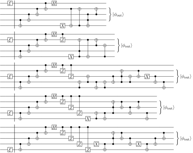
Figure 3: From top to bottom, the quantum circuits on the right side of the double vertical lines are for decoding and correcting the errors happening on qubits $1$–$5$, respectively. $\mathcal{E}$ on the left side of the double vertical lines denotes the error operation.

For each location of the error (on one of the five qubits), a different decoding circuit is needed. These five decoding circuits are shown in Figure 3, for correcting errors happening on qubits $1$–$5$, from top to bottom, respectively. The error operations, denoted as $\mathcal{E}$, are also shown in the decoding circuits, separated by the double vertical lines, noting that $\mathcal{E}$ can be an arbitrary unitary as well as non-unitary operation.

We consider arbitrary unitary errors which can be represented as

$$\mathcal{E}=e^{i\alpha}R_{\hat{n}}(\theta).$$ (3)

Here $R_{\hat{n}}(\theta)=e^{-i\theta\hat{n}\cdot\vec{\sigma}/2}$ denoting a rotation by $\theta$ along the $\hat{n}$ axis, where $\vec{\sigma}$ denotes a vector with three components formed by the Pauli matrices $X$, $Y$ and $Z$.

When the input state is chosen as

$$|\psi_{b}\rangle=|0\rangle_{1}|b\rangle_{234}|0\rangle_{5},$$ (4)

the output state after decoding has the form

$$|\Psi_{b}\rangle=|\Phi\rangle_{15}|b\rangle_{234},$$ (5)

which recovers the input state $|b\rangle$ of qubits $2$–$4$. The syndrome state $|\Phi\rangle_{15}$ contains information on the error.

Expanding the unitary $\mathcal{E}$ given in Eq. (3) as a linear combination of the matrices $E$, $X$, $Z$, and $Y$ gives

$$\mathcal{E}=c_{00}E+c_{01}X+c_{10}Z+c_{11}Y.$$ (6)

Here $E$ is the identity operator acting on a qubit, and

$$c_{00} {}=e^{i\alpha}\cos(\theta/2), c_{01} {}=-ie^{i\alpha}\sin(\theta/2)n_{x},$$

$$c_{10} {}=-ie^{i\alpha}\sin(\theta/2)n_{z},\quad\text{and}\quad c_{11} {}=-ie^{i\alpha}\sin(\theta/2)n_{y},$$

where $\hat{n}=(n_{x},n_{x},n_{z})$. We then obtain the syndrome part $|\Phi\rangle_{15}$ as

$$|\Phi\rangle_{15}=c_{00}|00\rangle+c_{01}|01\rangle+c_{10}|10\rangle+c_{11}|11\rangle.$$ (7)

III Experimental Protocol

Our experiment uses a Bruker DRX 700 MHz spectrometer. We choose ¹³C-labelled trans-crotonic acid dissolved in d6-acetone as the qubit system knill ; magic . The structure of the molecule is shown as the inset in Figure 4. The methyl group (denoted as M) can be treated as a spin half nucleus using a gradient-based subspace selection knill . The Hamiltonian of the seven spins can be represented as ($\hbar=1$)

$$H_{NMR}=\sum_{i}\pi\nu_{i}Z_{i}+\sum_{i<j}\frac{\pi}{2}J_{ij}Z_{i}Z_{j}$$ (8)

where $\nu_{i}$ denotes the chemical shift of spin $i$, and $J_{ij}$ denotes the scalar coupling strength between spins $i$ and $j$. The values of $\nu_{i}$, $J_{ij}$, and relaxation times are listed in Figure 4. We exploit the seven spins as seven qubits in experiment.

We prepare a labelled pseudopure state $\rho_{s}=\mathbf{0}\mathbf{0}Z\mathbf{0}\mathbf{0}\mathbf{0}\mathbf{0}$ using the method in Ref. knill . Here the labelled qubit is in state $Z$ and the other qubits are in state $\mathbf{0}=|0\rangle\langle 0|$. From left to right, the order of the spins is M, H₁, H₂, C₁, C₂, C₃, C₄. One should note that we are using the deviation density matrix formalism ChuangRoy . In experiment we do not use spins H₁ and H₂ in implementing the QECC, after the preparation of the state $\rho_{s}$. These two spins are only affected by the hard refocusing pulses. We therefore concentrate on the subsystem of the five spins M, C₁–C₄, denoted as qubits $1$–$5$, in which the QECC is implemented. Using some basic results on quantum circuits PRA95 ; ChuangAPL , we transform the circuits for implementing the QECC shown in Figures 2 and 3 into pulse sequences, shown in Figures 9 and 10 in the Appendix for encoding and decoding, respectively. The single-spin rotations along $z$-axis are implemented through the evolution of the chemical shifts in the Hamiltonian of the spin system Grape2 . Rotations along $x$- and $y$-axes are implemented by standard Isech-shaped r.f. pulses Grape2 ; isech1 ; isech2 for spins M and C₁, and pulses generated by the gradient ascent pulse engineering (GRAPE) algorithm Grape1 for C₂–C₄. The evolutions of the $J$-couplings between the neighboring qubits are implemented by numerically optimized refocusing pulses, which are standard Isech and Hermite-shaped r.f. pulses Grape2 ; Hermite and are not shown here. We choose artificial errors RayPRL01 ; Nature04ion to demonstrate the QECC, i.e., the error operations $\mathcal{E}$ in Eq. (3) are generated by r.f. pulses. All operations are combined in a custom-built software compiler to minimize error accumulation Grape2 ; magic .

We protect the quantum coherence to demonstrate the QECC by putting one qubit of the input state in a superposition $|+\rangle\equiv(|0\rangle+|1\rangle)/\sqrt{2}$. The corresponding coherence can be observed directly in the spectra of the input state and the final state after the completion of QECC (see below). We avoid the full quantum state tomography, which would make the demonstration more difficult because of the required additional experiments and the limitation of the spectral resolution of certain spins. We choose three input states as

$$|\psi_{k}\rangle=|0\rangle|s_{k}\rangle|0\rangle$$ (9)

with

$$|s_{1}\rangle=|+\rangle|00\rangle,\quad|s_{2}\rangle=|01\rangle|+\rangle,\quad|s_{3}\rangle=|00\rangle|+\rangle,$$ (10)

noting that all the basis states in Eq. (1) are included here. We introduce error operations of $X$-, $Y$- and $Z$-type by setting $\hat{n}$ in Eq. (3) along the $x$-, $y$-, and $z$-axes, respectively, and choose $\alpha=0$. Using Eq. (5) one can obtain the output states represented as

$$|\Psi_{k}\rangle=[\cos(\theta/2)|00\rangle_{15}-i\sin(\theta/2)|jl\rangle_{15}]\otimes|s_{k}\rangle_{234},$$ (11)

where $|jl\rangle=|01\rangle$, $|10\rangle$, and $|11\rangle$ for $X$-, $Z$-, and $Y$-type errors, respectively. Obviously one can obtain the results for the case of no error ($E$-type error) by setting $\theta=0$ in the above equation.

In NMR experiments, we can detect the states of the qubits through measuring the bulk magnetization spindynamics ; LARay

$$M(t)\propto{\rm Tr}[\rho(t)\sum_{j}(X_{j}+iY_{j})e^{-t/T_{2,j}^{*}}].$$ (12)

Here $\rho(t)=U(t)\rho(0)U^{\dagger}(t)$ where $U(t)=e^{-itH_{NMR}}$, and $\rho(0)$ denotes the density matrix of the state to be measured after the r.f. pulses are switched off. $T_{2,j}^{*}$ denotes the effective transverse relaxation time of spin $j$. One can obtain the NMR spectrum through the Fourier transform of $M(t)$. From some calculations, one can find that the single coherence elements in $\rho(0)$ can be directly measured in the spectrum, and the peaks of a certain spin are associated with the states of the other spins because of the $J$-couplings.

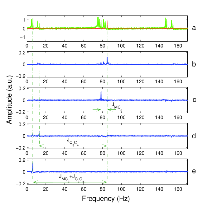
Figure 5: (Color online) Experimental NMR spectra of C₃ to illustrate the results for correcting Pauli errors. In figure (a) the spectrum shown as the thin curve is obtained from the input state $|\psi_{2}\rangle=|0\rangle|01\rangle|+\rangle|0\rangle$. The spectrum shown as the thick curve is obtained from the state of the equal weight superposition of all the computational basis states, with an applied scale factor of 16 for better visualization. Figures (b)–(e) illustrate the results of error correction for $E$, $Z$, $X$, and $Y$ errors, respectively. The shifts of the main peaks, which are indicated by the arrows, characterize the type of errors.

We first take spectra of C₁ for input $|\psi_{1}\rangle$, and spectra of C₃ for $|\psi_{2}\rangle$ and $|\psi_{3}\rangle$, respectively. There is only one peak in each spectrum, coming from the state $|0\rangle|+\rangle|000\rangle$, $|001\rangle|+\rangle|0\rangle$, or $|000|+\rangle|0\rangle$, in the input state $|\psi_{1}\rangle$, $|\psi_{2}\rangle$, or $|\psi_{3}\rangle$, respectively, illustrated by the spectrum shown as the solid curve in Figure 5 (a) obtained from $|\psi_{2}\rangle$. The amplitude of the peak is proportional to the element of the quantum coherence to be protected in state $|s_{k}\rangle$ in Eq. (10) against the error operations $\mathcal{E}$. We take the amplitude of the peak in the spectrum obtained from the input state as the reference to normalize the corresponding output signals after completion of the QECC procedure.

In principle, full quantum process tomography (QPT) is required to completely evaluate the implementation of the QECC and analyze experimental errors. Based on the result of the QPT, one can estimate the experimental errors of the quantum gates for implementing the QECC through proper models for relaxation effects bookChuang . In practice, however, this task is rather difficult because the number of experiments required for the QPT increases exponentially with the involved qubits. In our five qubit case, more than one million ($4^{2n}-4^{n}=4^{10}-4^{5}$) real numbers have to be determined SEQPT11 . Moreover, the limitation of the spectral resolution of certain spins in our molecule further increases the difficulty. More recent strategies for characterizing quantum processes SEQPT11 ; PCQD might allow an improved evaluation of our QEC procedure. Here we choose a simplified approach to demonstrate robustness of the scheme against artificially introduced errors, and estimate experimental errors in combination with simulation results.

Noting that in Eq. (11) the two syndrome qubits are not entangled with the register qubits, one can extract the state of the register by tracing over the syndrome qubits in $|\Psi_{k}\rangle\langle\Psi_{k}|$. In experiment we only take the spectra of the register qubits, and implement the partial trace by adding the splitting of the peaks of the register qubits caused the coupling of the syndrome qubits. Through Eq. (11), one finds that the state $|0\rangle|+\rangle|000\rangle$, $|001\rangle|+\rangle|0\rangle$, or $|000\rangle|+\rangle|0\rangle$ contributes a peak with amplitude

$$A_{0} = \cos^{2}(\theta/2),$$ (13)

and $|j\rangle|+\rangle|00l\rangle$, $|j\rangle|01\rangle|+\rangle|l\rangle$, or $|j00\rangle|+\rangle|l\rangle$ contributes a peak with amplitude

$$A_{1} = \sin^{2}(\theta/2)$$ (14)

in the state $|\Psi_{1}\rangle$, $|\Psi_{2}\rangle$, or $|\Psi_{3}\rangle$, respectively, after the completion of the QECC, where the sum $A_{0}+A_{1}=1$ shows the robustness against the error operations. We can therefore benchmark the QECC procedure through measuring $A_{0}$ and $A_{1}$. Moreover one can obtain the rotation angle $\theta$ through $A_{0}$ and $A_{1}$ up to its sign. One should notice that we do not measure the syndrome qubits directly. The NMR spectrum of the output state is not necessary exactly in phase with the reference spectrum, due to experimental errors, e.g. imperfection of r.f. pulses. We therefore choose the absolute values $I_{0}=|A_{0}|$, $I_{1}=|A_{1}|$, and $I=|A_{0}+A_{1}|$ to represent the results.

IV Experimental results

We summarize our experimental results in this section. We have implemented the $((5,5,2))$ code in three different situations, for different input states and artificial errors.

Setting A. A single input state $|\psi_{2}\rangle$ as given in Eq. (9), and Pauli errors $X$, $Y$, $Z$, and $E$ on each of the five qubits. The results are summarized in subsection A.

Setting B. A single input state $|\psi_{2}\rangle$ as given in Eq. (9), and arbitrary $X$-, $Y$-, and $Z$-type errors, i.e., arbitrary rotations by an angle $\theta$ along the $x$-, $y$-, and $z$-axes. We analyze the information on the rotation angle $\theta$ and sumamrize the results in subsection B.

Setting C. Three input states $|\psi_{1}\rangle,|\psi_{2}\rangle,|\psi_{3}\rangle$ as given in Eq. (9), and arbitrary rotation errors along the $y$-axis. The results are summarized in subsection C.

For all three situations, our results clearly demonstrate quantum coherence for implementing the QECC procedure.

IV.1 A. Correcting Pauli errors

Figure 5 shows the experimental NMR spectra of C₃ to illustrate the results for correcting Pauli errors, i.e., $E$, $Z$, $X$, and $Y$ errors. In Figure 5 (a) the spectrum shown as the thin curve is the reference spectrum, obtained from the input state $|\psi_{2}\rangle=|0\rangle|01\rangle|+\rangle|0\rangle$. The spectrum shown as the thick curve is obtained from the state of the equal weight superposition of all the computational basis states (i.e. $|+\rangle|+\rangle|+\rangle|+\rangle|+\rangle$), where a scale factor of 16 is applied for better visualization. One can exploit the positions of the peaks in this spectrum for facilitating to locate the peaks in other spectra. Figures 5 (b)–(e) illustrate the results of error correction for $E$, $Z$, $X$, and $Y$ errors, respectively. The shifts of the main peaks characterize the type of errors. The distance of the shifts, measured in $J$-couplings, is indicated by the arrows.

IV.2 B. Correcting $X$-, $Y$-, and $Z$-type errors

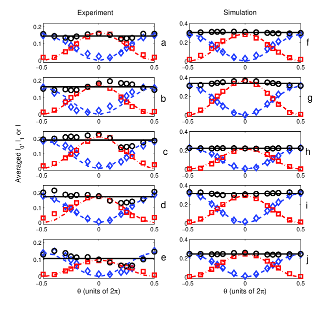
Figure 6: (Color online) Averaged results of the correction for $X$-, $Y$- and $Z$-type errors. The input state is chosen as $|\psi_{2}\rangle$, and the signal in the input state is chosen as reference to normalize the signals after the completion of the QECC procedure. The left and right columns show the results in experiment and by simulation, respectively. The results for errors on qubits $1$–$5$ are shown from top to bottom, respectively. The averaged $I_{0}$ and $I_{1}$, denoted as $\bar{I}_{0}$ and $\bar{I}_{1}$, are indicated by squares and diamonds, respectively. In comparison with the theoretical values $\bar{I}_{0}^{th}$ and $\bar{I}_{1}^{th}$, the data can be fitted as $\alpha_{0}\bar{I}_{0}^{th}$ and $\alpha_{1}\bar{I}_{1}^{th}$ shown as the dash-dotted and dashed curves in figures (a)–(e) for experiment and (f)–(j) for simulation, where $\alpha_{0}$ and $\alpha_{1}$ are constant coefficients in each figure and listed in the main text. The averaged $I$, denoted as $\bar{I}$ and marked as circles, indicates the intensity of the remaining signals after completion of the QECC procedure. The remaining signal is robust against the rotation angle $\theta$, demonstrating the success of the QEC procedure.

The input state is chosen as $|\psi_{2}\rangle$. The results for correcting $X$-, $Y$-, and $Z$-type errors with arbitrary rotations are shown in Figure 6. We exploit the averaged $I_{0}$, $I_{1}$ and $I$, respectively denoted as $\bar{I}_{0}$, $\bar{I}_{1}$ and $\bar{I}$, over the results of correcting the three types of errors as benchmark. The experimental results for correcting errors on qubits $1$–$5$ are shown as Figures 6 (a)–(e), respectively, where $\bar{I}_{0}$, $\bar{I}_{1}$, and $\bar{I}$ are indicated by squares, diamonds and circles. In comparison with the theoretical values $\bar{I}_{0}^{th}$ and $\bar{I}_{1}^{th}$, the experimental data can be fitted as $\alpha_{0}\bar{I}_{0}^{th}$ and $\alpha_{1}\bar{I}_{1}^{th}$ shown as the dash-dotted and dashed curves. We fit the data for $\bar{I}$ using a constant function, shown as the plane lines. The remaining quantum coherence is robust against the rotation angle $\theta$, demonstrating the success of the QECC procedure. The values of the fitted $\alpha_{0}$, $\alpha_{1}$ and $\bar{I}$ are listed in Table 1. We also list the results by simulation in Figures 6 (f)–(j), for correcting the errors happening on qubits $1$–$5$, respectively. In simulation, we take into account the $T_{2}$ effects, imperfection in refocusing protocols and the theoretical infidelity of the numerically generated pulses. The fitting results for $\alpha_{0}$, $\alpha_{1}$ and $\bar{I}$ are also listed in Table 1.

Error location	1	2	3	4	5
$\alpha_{0}$ (experiment)	$0.156\pm 0.020$	$0.160\pm 0.038$	$0.191\pm 0.036$	$0.177\pm 0.010$	$0.142\pm 0.038$
$\alpha_{1}$ (experiment)	$0.168\pm 0.023$	$0.176\pm 0.019$	$0.215\pm 0.025$	$0.177\pm 0.038$	$0.099\pm 0.016$
$\bar{I}$ (experiment)	$0.146\pm 0.012$	$0.164\pm 0.018$	$0.193\pm 0.028$	$0.174\pm 0.027$	$0.107\pm 0.029$
$\alpha_{0}$ (simulation)	$0.288\pm 0.031$	$0.312\pm 0.018$	$0.230\pm 0.016$	$0.322\pm 0.019$	$0.249\pm 0.015$
$\alpha_{1}$ (simulation)	$0.295\pm 0.037$	$0.369\pm 0.022$	$0.218\pm 0.020$	$0.295\pm 0.016$	$0.250\pm 0.013$
$\bar{I}$ (simulation)	$0.304\pm 0.007$	$0.337\pm 0.018$	$0.222\pm 0.003$	$0.315\pm 0.010$	$0.246\pm 0.006$

Table 1: The fitted $\alpha_{0}$, $\alpha_{1}$ and $\bar{I}$ in experiment and by simulation in case B.

IV.3 C. Correcting $Y$-type errors from various input states

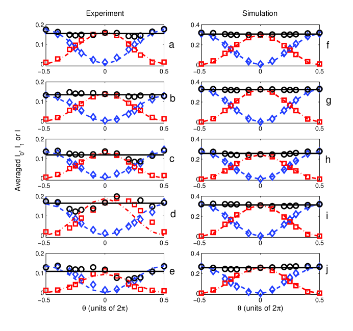
Figure 7: (Color online) Averaged results over various input states $|\psi_{k}\rangle$ ($k=1,2,3$) for correcting $Y$-type errors. The left and right columns show the results in experiment and by simulation, respectively. The results for errors on qubits $1$–$5$ are shown from top to bottom, respectively. We choose the signals of the input states as reference to normalize the signals after the completion of the QECC procedure. $\bar{I}_{0}$ and $\bar{I}_{1}$ are indicated by squares and diamonds, respectively. In comparison with the theoretical values $\bar{I}_{0}^{th}$ and $\bar{I}_{1}^{th}$, the data can be fitted as $\alpha_{0}\bar{I}_{0}^{th}$ and $\alpha_{1}\bar{I}_{1}^{th}$ shown as the dash-dotted and dashed curves in figures (a)–(e) for experiment and (f)–(j) for simulation, where $\alpha_{0}$ and $\alpha_{1}$ are listed in the main text. The intensity $\bar{I}$ of the remaining signal, marked as circles, is robust against the rotation angle $\theta$, demonstrating the success of the QEC procedure.

We measure $I_{0}$, $I_{1}$, and $I$ for the three input states $|\psi_{k}\rangle$ with $k=1$, $2$, $3$, and exploit the average over the input states, respectively denoted as $\bar{I}_{0}$, $\bar{I}_{1}$ and $\bar{I}$, to represent the results of the error correction. The results in the experimental implementation and by simulation are shown in Figures 7 (a)–(e), and (f)–(j), corresponding to errors happening on qubits $1$–$5$, respectively, where $\bar{I}_{0}$, $\bar{I}_{1}$ and $\bar{I}$ are indicated by squares, diamonds and circles. In comparison with the theoretical values $\bar{I}_{0}^{th}$ and $\bar{I}_{1}^{th}$, the experimental data can be fitted as $\alpha_{0}\bar{I}_{0}^{th}$ and $\alpha_{1}\bar{I}_{1}^{th}$ shown as the dash-dotted and dashed curves in Figures 7 (a)–(e). The data for $\bar{I}$ can be fitted as a constant function, and the fitting results are shown as the plane lines. The remaining quantum coherence is robust against the rotation angle $\theta$, demonstrating the success of the QECC procedure. The values of the fitted $\alpha_{0}$, $\alpha_{1}$ and $\bar{I}$ for the results in experiment and by simulation are listed in Table 2.

Error location	1	2	3	4	5
$\alpha_{0}$ (experiment)	$0.175\pm 0.013$	$0.130\pm 0.011$	$0.136\pm 0.012$	$0.161\pm 0.022$	$0.137\pm 0.026$
$\alpha_{1}$ (experiment)	$0.165\pm 0.017$	$0.140\pm 0.010$	$0.128\pm 0.010$	$0.188\pm 0.063$	$0.093\pm 0.019$
$\bar{I}$ (experiment)	$0.155\pm 0.012$	$0.134\pm 0.007$	$0.119\pm 0.018$	$0.165\pm 0.027$	$0.108\pm 0.024$
$\alpha_{0}$ (simulation)	$0.314\pm 0.008$	$0.330\pm 0.002$	$0.276\pm 0.005$	$0.324\pm 0.008$	$0.269\pm 0.031$
$\alpha_{1}$ (simulation)	$0.301\pm 0.012$	$0.327\pm 0.005$	$0.243\pm 0.005$	$0.311\pm 0.017$	$0.260\pm 0.016$
$\bar{I}$ (simulation)	$0.307\pm 0.008$	$0.323\pm 0.004$	$0.257\pm 0.014$	$0.314\pm 0.008$	$0.258\pm 0.011$

Table 2: The fitted $\alpha_{0}$, $\alpha_{1}$ and $\bar{I}$ in experiment and by simulation in case C.

V Discussion of the experimental results

V.1 A. Extracting partial information of error operations

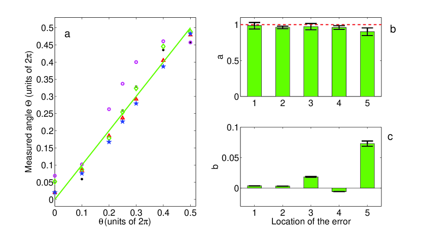
Figure 8: (Color online) Experimental results of error syndromes. Using the measured $\bar{I}_{0}$ and $\bar{I}_{1}$, we obtain the absolute values of the rotation angles for the errors, denoted by $\Theta$. The theoretical expectation $\Theta=\theta$ is shown as the line. The experimental data for errors happening on qubits $1$–$5$ are denoted as filled circles, triangles, diamonds, stars, and empty circles, respectively. The deviation of the data for errors happening at qubit 5 is larger than the other cases, because more r.f. pulses are required for correcting the errors at qubit 5 (see Figure 10). We exploit $\Theta=a\theta+b$ to fit the data. The coefficients $a$ and $b$ are shown in figure (b) and (c), respectively, where the dashed line indicates the theoretical value $a=1$.

Through measuring the qubits of the register [see Eqs. (13) and (14)], we can obtain partial information of the errors, i.e., the types of the errors illustrated in Figure 5, and the absolute values of the rotation angles of the errors, exploiting the couplings between the register and syndrome qubits. Figure 8 illustrates the experimental results obtained from the data in Figure 7 for extracting absolute values of the rotation angles. In Figure 8 (a), the theoretical expectation $\Theta=\theta$ is shown as the line. The experimental data is distributed near the line. We fit the data using a linear function as $\Theta=a\theta+b$. The coefficients $a$ and $b$ are shown in Figure 8 (b) and (c), respectively, where the dashed line indicates the theoretical value of $a=1$. The fitting results show a good agreement between experiment and theory.

V.2 B. Error sources in implementation

The simulation is mainly used to analyze experimental errors. Excluding the preparation of the pseudopure state, the number of r.f. pulses ranges from about $320$ to $440$, and the duration of the experiments ranges from about $0.55$s to $0.72$s. The duration is comparable with, and indeed very close to the transverse relaxation times ($T_{2}$’s in Figure 4). Hence the limitation of the coherence time contributes major experimental errors. Through comparing the results by simulation with and without $T_{2}$ effects, we estimate that the limitation of $T_{2}$ contributes to about $34\%$–$45\%$ of the loss of signal. Additionally, the errors due to imperfections of the refocusing protocols and the implementation of r.f. pulses contribute about $10\%$–$16\%$ and $3\%$–$19\%$ of the loss of signal, respectively.

V.3 C. Comparison with the implementation of the $((5,2^{1},3))$ code

We use the same seven-spin-qubit NMR system that was used in the implementation of the $((5,2^{1},3))$ codes RayPRL01 . It should be emphasized that in the $((5,2^{1},3))$ experiment, the entire circuit one would need to carry out consists of four parts: encoding, (artificial) errors, decoding, and recovery. The decoding circuit is just the reverse of the encoding circuit, but the recovery circuit involves approximately three times more gates than the encoding/decoding circuit. However, because the artificial errors demonstrated for the code $((5,2^{1},3))$ are all Pauli errors, after the decoding circuit using only Clifford gates (gates that map Pauli operators to Pauli operators), the five qubits are in a product state. Only a single qubit carries information that needs a recovery operation, while the other four qubits carry error syndrome information. Consequently, the noise (mainly dephasing noise) during the recovery procedure does not have much effect on the final experimental fidelity, as coherence is only needed to be maintained on a single qubit.

On the contrary, we use three qubits to carry information. Although our experiment requires implementing quantum circuits some of which are of comparable size as those for the $((5,2^{1},3))$ code, quantum coherence in a larger Hilbert space has to be maintained throughout the entire procedure of the code. In implementation, maintaining coherence in a larger space e.g. three qubits, is more difficult than in a one-qubit space, because the high order coherence could decay faster than the single coherence under effects of decoherence CoryNMRQC . This case might explain the low remaining signals in our experiment ($10$–$20\%$), compared with the $((5,2^{1},3))$ experiment where the intensity of the remaining signals ranges $48$–$87\%$.

VI Conclusion

We implement a five-qubit quantum error-correcting code using NMR. The code protects an arbitrary state in a five-dimensional Hilbert space, and is capable of correcting a single erasure error. The code is a CWS code which encodes a larger Hilbert space than any stabilizer code with the same length and being capable of correcting a single erasure error. Our results demonstrate a good nonadditive quantum code in experiment for the first time.

Compared with the previous implementation of another five-qubit code using the same seven-spin-qubit system RayPRL01 , which encodes a two-dimensional Hilbert space and is capable of correcting an arbitrary single-qubit error, the pulse sequences in our experiment are more complex. In order to shorten the length of sequences, we exploit pulses optimized by the GRAPE algorithm to implement the $\pi/2$ spin-selective pulses for certain spins. The duration of our experiments ranges from $0.55$s to $0.72$s, which challenges the ultimate limit of coherent control of the system, with a typical $T_{2}$ time ranging from $0.8$s to $1.1$s. Despite experimental imperfections which induce signal loss, the signal remains resilient against the artificial errors.

Figure 1: Outline of the protocol for the QECC procedure. Five qubits $1$–$5$ are represented by five lines, from top to bottom, where qubits $2$, $3$, and $4$ are exploited to carry the input state $|\phi_{\text{in}}\rangle_{234}$, and qubits $1$ and $5$ are syndrome qubits. The error can happen on any of the five qubits. The decoding operation depends on the location of the error. In the ideal case the output state obeys $|\phi_{\text{out}}\rangle=|\phi_{\text{in}}\rangle$.

Figure 2: Quantum circuit for encoding. Elements $\oplus$ and $\bullet$ connected by a line denote a controlled-NOT or Toffoli gate conditioned on the state $|1\rangle$. $X$ denotes the Pauli matrix $\sigma_{x}$, acting as a NOT gate, and $H$ denotes a Hadmard gate.

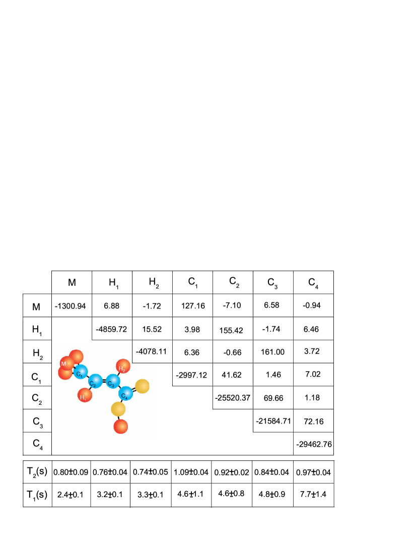
Figure 4: (Color online) Characteristics of the molecule of trans-crotonic acid. The molecular structure is shown as the inset. The chemical shifts and $J$-coupling constants (in Hz) are on and above the diagonal in the table. The longitudinal and transversal relaxation times $T_{1}$ and $T_{2}$, which are listed at the bottom, are estimated by the standard inversion recovery and Hahn echo sequences. The chemical shifts are given with respect to reference frequencies of 700.13 MHz (protons) and 176.05 MHz (carbons). The nine weakly coupled spin half nuclei can provide seven qubits since the methyl group can be treated as a single qubit using a gradient-based subspace selection knill .

Figure 9: Pulse sequences to encode the $((5,5,2))$ code.

Figure 10: Pulse sequences to decode the $((5,5,2))$ code, for errors happening on each of the five qubits.

References

- (1) M. Nielsen and I. Chuang, Quantum Computation and Quantum Information (Cambridge University Press, Cambridge, 2000).
- (2) E. Knill, R. Laflamme and W. H. Zurek, Science, 279, 342 (1998); A. Yu. Kitaev, Russ. Math. Surv. 52, 1191(1997).
- (3) D. Aharonov and M. Ben-Or, Proceedings of the 29th Annual ACM Symposium on Theory of Computing, 176, ACM Press, (1997).
- (4) E. Knill, Nature, 434, 39 (2005).
- (5) D. Gottesman, Encyclopedia of Mathematical Physics, edited by J.-P. Francoise, G. L. Naber, and S. T. Tsou, 196, Elsevier, Oxford, (2006).
- (6) D. Gottesman, quant-ph/9705052, Caltech Ph.D. thesis.
- (7) A. R. Calderbank, E. M. Rains, P. W. Shor, and N. J. A. Sloane, IEEE Transactions on Information Theory, 44, 1369 (1998).
- (8) In this article, we restrict ourselves to qubit systems, but the theory of QECCs can be applied to systems of arbitrary dimension.
- (9) M. Grassl, T. Beth, and T. Pellizzari, Phys. Rev. A 56, 33 (1997).
- (10) L. Vaidman, L. Goldenberg, and S. Wiesner, Phys. Rev. A 54, R1745 (1996).
- (11) R. Laflamme, C. Miquel, J. P. Paz, and W. H. Zurek, Phys. Rev. Lett. 77, 198 (1996).
- (12) C. H. Bennett, D.P. DiVincenzo, J. A. Smolin, and W. K. Wootters, Phys. Rev. A 54 3824 (1996).
- (13) E. M. Rains, R. H. Hardin, P. W. Shor, and N. J. A. Sloane, Phys. Rev. Lett. 79, 953 (1997).
- (14) J. A. Smolin, G. Smith, S. Wehner, Phys. Rev. Lett. 99, 130505 (2007).
- (15) S. Yu, Q. Chen, C. H. Lai, and C. H. Oh, Phys. Rev. Lett. 101, 090501 (2008).
- (16) A. Cross, G. Smith, J. A. Smolin, and B. Zeng, IEEE Transactions on Information Theory, 55 (1), 433 (2009).
- (17) M. Grassl and M. Rotteler, Proc. 2008 IEEE Int. Symp. Inform. Theory, pp. 300–304 (2008). arXiv: 0801.2150.
- (18) M. Grassl and M. Rotteler, Proc. 2008 IEEE Inf. Theory Workshop, pp. 396–400 (2008). arXiv: 0801.2144.
- (19) M. Grassl, P. W. Shor, G. Smith, J. Smolin, and B. Zeng, Physical Review A 79, 050306(R) (2009).
- (20) M. Grassl, P. W. Shor, and B. Zeng, Proc. 2009 IEEE Int. Symp. Inform. Theory, pp. 953–957 (2009).
- (21) D. Hu, W. Tang, M. Zhao, Q. Chen, S. Yu, and C. H. Oh, Phys. Rev. A 78, 012306 (2008).
- (22) S. Yu, Q. Chen, and C. H. Oh, arXiv:0901.1935.
- (23) C.-Y. Lu et al., Proc. Natl. Acad. Sci. USA 105, 11050 (2008).
- (24) E. Knill, R. Laflamme, R. Martinez, and C. Negrevergne, Phys. Rev. Lett. 86, 5811 (2001).
- (25) L. M. K. Vandersypen and I. L. Chuang, Rev. Mod. Phys., 76, 1037 (2004).
- (26) E. Knill et al., Nature, 404, 368 (2000).
- (27) A. M. Souza et al., Nat. Commun. 2: 169 doi: 10.1038/ncomms1166 (2011).
- (28) I. L. Chuang, N. Gershenfeld, M. G. Kubinec, and D. W. Leung, Proc. R. Soc. London, Ser. A 454, 447 (1998).
- (29) A. Barenco, C. H. Bennett, R. Cleve, D. P. DiVincenzo, N. Margolus, P. Shor, T. Sleator, J. A. Smolin, and H. Weinfurter, Phys. Rev. A 52, 3457–3467 (1995).
- (30) L. M. K. Vandersypen, M. Steffen, M. H. Sherwood, C. S. Yannoni, G. Breyta, and I. L. Chuang, Appl. Phys. Lett. 76, 646 (2000).
- (31) C. A. Ryan et al., Phys. Rev. A 78, 012328 (2008).
- (32) M. S. Silver, R. I. Joseph, C.-N. Chen, V. J. Sank and D. I. Hoult, Nature (London) 310, 681 (1984).
- (33) M. S. Silver, R. I. Joseph, and D. I. Hoult, Phys. Rev. A 31, 2753 (1985).
- (34) N. Khaneja et al., J. Magn. Reson. 172, 296 (2005).
- (35) W. S. Warren, J. Chem. Phys. 81, 5437 (1984).
- (36) J. Chiaverini et al., Nature (London) 432, 602 (2004).
- (37) M. H. Levitt, Spin Dynamics (John Wiley & Sons Ltd, West Sussex, England, 2008).
- (38) R. Laflamme et al., Los Alamos Science (Number 27), 226 (2002).
- (39) C. T. Schmiegelow, A. Bendersky, M. A. Larotonda, and J. P. Paz, Phys. Rev. Lett. 107, 100502 (2011).
- (40) M. P. Silva, O. Landon-Cardinal, and D. Poulin, Phys. Rev. Lett. 107, 210404 (2011).
- (41) T. F. Havel et al., Appl. Algebra Eng. Commun. Comput. 10, 339 (2000).