Branching Ratio of the Electromagnetic Decay of the $\Sigma^{+}(1385)$

Abstract

The CLAS detector was used to obtain the first ever measurement of the electromagnetic decay of the $\Sigma^{*+}(1385)$ from the reaction $\gamma p\to K^{0}\Sigma^{*+}(1385)$. A real photon beam with a maximum energy of 3.8 GeV was incident on a liquid-hydrogen target, resulting in the photoproduction of the kaon and $\Sigma^{*}$ hyperon. Kinematic fitting was used to separate the reaction channel from the background processes. The fitting algorithm exploited a new method to kinematically fit neutrons in the CLAS detector, leading to the partial width measurement of $250.0\pm 56.9(stat)^{+34.3}_{-41.2}(sys)$ keV. A U-spin symmetry test using the SU(3) flavor-multiplet representation yields predictions for the $\Sigma^{*+}(1385)\to\Sigma^{+}\gamma$ and $\Sigma^{*0}(1385)\to\Lambda\gamma$ partial widths that agree with the experimental measurements.

I Introduction

The electromagnetic (EM) decay of baryons can provide considerable information on their underlying structure. This transition offers a clean probe of the wavefunction of the initial and final state baryons, providing theoretical constraints and tests of the quark model. The non-relativistic quark model (NRQM) of Isgur and Karl Isgur1 ; Isgur2 predicts the electromagnetic properties of the ground state baryons reasonably well. It has been less successful giving accurate descriptions of the low-lying excited-state hyperons. Several other theoretical techniques have been used to more accurately calculate these transitions, including (NRQM) DHK ; Koniuk , a relativized constituent quark model (RCQM) warns , a chiral constituent quark model ($\chi$CQM) wagner , the MIT bag model kaxiras , the bound-state soliton model Schat , a three-flavor generalization of the Skyrme model that uses the collective approach Abada ; Haberichter , and an algebraic model of hadron structure Bijker .

Photoproduction from nucleon targets is a useful technique to cleanly generate a significant statistical sample of hyperons and to measure EM transitions to other decuplet baryons. If the EM transition form factors for decuplet baryons with strangeness are also sensitive to meson cloud effects, models attempting to make predictions of the decuplet radiative decay widths will need revisions to incorporate this effect. Comparison of data for the EM decay of decuplet hyperons, $\Sigma^{*}$, to the present predictions of quark models provides a measure of the importance of meson cloud diagrams in the $\Sigma^{*}\to Y\gamma$ transition. Experimental results for the EM decay ratios for all $\Sigma^{*}$ charge states are desirable to obtain a complete comparison to EM decay predictions for the $\Sigma^{*}$. Precision measurements of the $\Sigma^{*-}\to\Sigma^{-}\gamma$ and $\Sigma^{*+}\to\Sigma^{+}\gamma$ decay widths can be particularly useful in determining the degree of SU(3) symmetry breaking.

The decay width from the measurement of $\Sigma^{*0}\to\Lambda\gamma$ kellpaper ; taylor is much larger than most current theoretical predictions. This could be due to meson cloud effects, which were not included in these calculations. There is a theoretical basis for calculating these effects Lee that suggests pion cloud effects may be sizable. For example, they are predicted to contribute on the order of $\sim$40% to the $\gamma p\to\Delta^{+}$ magnetic dipole transition form factor, $G^{\Delta}_{M}(Q^{2})$, for low $Q^{2}$. The CQM CQM indicates that the value of $G^{\Delta}_{M}(0)$ is directly proportional to the proton magnetic moment Lee , and measurements of $G^{\Delta}_{M}$ for low $Q^{2}$ are rationalized in the framework of the model if the experimental magnetic moment is lowered by about 25%.

With theoretical predictions for the degree at which the meson cloud effects plays a role, it is then possible to test $SU(3)$ flavor symmetry breaking (and the degree at which it is broken). This can be achieved by measuring both the $\Gamma(\Sigma^{*-}\to\Sigma^{-}\gamma)$ and $\Gamma(\Sigma^{*+}\to\Sigma^{+}\gamma)$ decay widths and comparing these to predictions from flavor SU(3) relations.

Just like isospin invariance can be used to compare the $\Delta^{++}\to p\pi^{+}$ and $\Delta^{+}\to p\pi^{0}$ decays, U-spin invariance may be used to compare the $\Sigma^{*+}\to\Sigma^{+}\gamma$ and $\Delta^{+}\to p\gamma$ decays. U-spin is analogous to isospin in that it is a symmetry in the exchange of the $d$ and $s$ quarks rather than the $u$ and $d$ quarks. A value of U-spin can be assigned to each baryon based on its quark composition. The $\Sigma^{*-}$ and the $\Xi^{*-}$ of the baryon decuplet have $U=3/2$, whereas the octet baryons $\Sigma^{-}$ and $\Xi^{-}$ have $U=1/2$.

U-spin symmetry forbids radiative decays of specific decuplet baryons. Since the photon is a charge singlet with $U=0$, this implies that

$$\Sigma^{*-}\to\Sigma^{-}\gamma\ {\rm and}\ \Xi^{*-}\to\Xi^{-}\gamma$$

have zero amplitude in the equal-mass limit due to U-spin symmetry. This can also be understood in the context of the SU(6) wavefunctions for these baryons. The M1 transition operator is written between the initial and final states as :

$$\langle\Sigma^{-}_{SU(6)}|\,\sum_{q}\frac{Q_{q}}{2m_{q}}\sigma_{q}\cdot\left(\bf k\rm\times\epsilon^{*\lambda}\right)\,|\Sigma^{*-}_{SU(6)}\rangle=0.$$ (1)

Here the sum is over all $q$ constituent quarks, $m_{q}$, $\sigma_{q}$ and $Q_{q}$ are the mass, spin vector and charge of the $q$ quark, $\bf k\rm$ is the propagation direction, and $\epsilon^{*\lambda}$ is the polarization vector. One can also show that the same transition operator for the $\Sigma^{*+}$ gives a non-zero amplitude. U-spin invariance implies a large difference in the radiative decay widths of the $\Sigma^{*-}$ and $\Sigma^{*+}$.

The chiral symmetry for U-spin is strongly broken because the constituent mass of the strange quark, $m_{s}$, is approximately 1.5 times greater than the non-strange quarks, $m$. The magnetic moment is inversely proportional to the mass, and so there is no cancellation in the wavefunction like in the equal-mass $SU(6)$ case in Eq. 1. From Ref. lipkin2 , an estimate of the ratio of the EM decay rates from the ratio of the square of the transition operators can be expressed as

$$\frac{\Gamma(\Sigma^{*-}\to\Sigma^{-}\gamma)}{\Gamma(\Sigma^{*+}\to\Sigma^{+}\gamma)}\approx\frac{1}{9}\left(1-\frac{m}{m_{s}}\right)^{2},$$

resulting in a value of about 1%. This suggests that U-spin symmetry breaking for radiative decays is at the level of only a few percent. At this level U-spin is an effective tool, even considering the quark mass difference.

Detailed calculations from the CQM and $1/N_{c}$-type expansions of the EM decay rates have been carried out by several groups quarks ; nrqm , all of which come up with decay ratios of a similar scale. In lattice QCD, the quarks have very different interactions with the photon than for the CQM, but these too have ratios (for the above equation) within a few percent lattice . This consistency makes a stronger case for the usefulness of U-spin symmetry.

There has been much theoretical interest in radiative baryon decays. However, there are only a few measurements. Recently, a measurement of the radiative decay of the $\Sigma^{*-}$ was attempted by the SELEX collaboration selex , resulting in only an upper limit. The 90% confidence level upper bound of $\Gamma=9.5$ keV was reported, however most models predict a value of less than 4 keV. Ultimately this result has limited power to constrain theoretical estimates. More experimental measurements are necessary to provide better constraints.

A program to investigate the various $\Sigma^{*}$ electromagnetic decays is underway using data from the CEBAF Large Angle Spectrometer (CLAS) detector. First, two independent analyses of the EM decay of the $\Sigma^{*0}$ have been completed kellpaper , taylor . The consistency in these results has given confidence in the notion that meson cloud effects are indeed contributing significantly. The next step described and presented here was to measure the $\Sigma^{*+}$ electromagnetic decay, which has not been done before. The final program analysis for the $\Sigma^{*-}\to\Sigma^{-}\gamma$ decay will be addressed in a future CLAS publication.

In the following, a description of the experimental details and analysis procedure for extracting the $\Sigma^{*+}$ EM decay branching ratio normalized to the strong decay is provided. Some specifics are given about neutron detection and the development of the neutron covariance matrix required by the analysis. After the signal extraction a U-spin symmetry test using the U-spin SU(3) multiplet representation is used to predict the $\Sigma^{*+}\to\Sigma^{+}\gamma$ and $\Sigma^{*0}\to\Lambda\gamma$ partial widths, which are then compared to the experimental results.

II The Experiment

The present measurements were carried out with the CLAS in Hall B at the Thomas Jefferson National Accelerator Facility mecking . An electron beam of energy 4.023 GeV was used to produce a photon beam with an energy range of 1.6-3.8 GeV, as deduced by a magnetic spectrometer tagnim that “tagged” the electron with an energy resolution of $\sim 0.1\%$. A 40-cm-long liquid hydrogen target was placed such that the center of the target was 10 cm upstream from the center of CLAS.

The CLAS detector is constructed around six superconducting coils that generate a toroidal magnetic field to momentum-analyze charged particles. The detection system consists of multiple layers of drift chambers to determine charged-particle trajectories, Cerenkov detectors for electron/pion separation, scintillation counters for flight-time measurements, and calorimeters to identify electrons and high-energy neutral particles, see Fig. 1. The Cerenkov detectors are not required for this experiment.

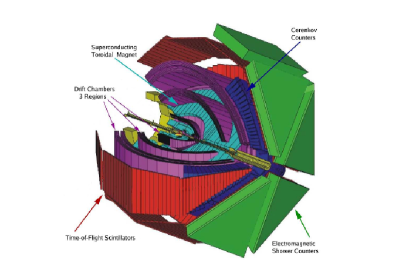
Figure 1: The CLAS detector at Jefferson Lab showing the toroidal magnet, the drift chambers, the time-of-flight scintillators, the cerenkov counter, and the electromagnetic calorimeter.

Each event trigger required a coincidence between the OR of the detector elements in the focal plane of the photon spectrometer and the CLAS Level 1 trigger. The Level 1 trigger required two charged particles in two different sectors of CLAS within a 150 ns coincidence time window. The approximate integrated luminosity for the CLAS $g11a$ run period used in this analysis was 70 pb^-1. Details of the experimental setup can be found in Refs. mecking ; mccracken .

III Event Selection

Events were selected for the channel $\gamma p\to K^{0}\Sigma^{*+}$. The present Particle Data Group (PDG) branching ratios list the decay $\Sigma^{*}\to\Sigma\pi$ to be $11.7\pm 1.5\%$, and assuming isospin symmetry, this leads to a branching ratio of $5.85\pm 0.75\%$ for the $\Sigma^{*+}\to\Sigma^{+}\pi^{0}$ decay pdg . This channel will be used to normalize the radiative signal that comes from the channel $\Sigma^{*+}\to\Sigma^{+}\gamma$. For both channels the topology of the decay is $\gamma p\to K^{0}\Sigma^{+}(X)$, where $X$ is not directly measured, such that the $\pi^{0}$ and $\gamma$ are differentiated using conservation of energy and momentum. This topology leads to the final set of decay products $\gamma p\to K^{0}\Sigma^{+}(X)\to\pi^{+}\pi^{-}\pi^{+}n(X)$. The charged particles can easily be detected with the use of the CLAS drift chambers and time-of-flight system. The neutron must be detected with the CLAS electromagnetic calorimeters. The analysis was done using a previously prepared data reduction (skim) that required two positively charged tracks and one negatively charged track for each event.

Cuts were applied to take into account both the regions of CLAS where there are holes in the acceptance that arose from problematic detector elements and regions that were not well simulated. This includes tracks at extremely forward or backward angles, areas near the torus coils, and regions where the drift chambers and scintillator counter efficiencies were not well understood. Tracks that point near these shadow regions are less likely to be reconstructed accurately. In addition a minimum momentum of 0.125 GeV, after energy loss corrections, was enforced for both positively and negatively charged particles to ensure accurate drift chamber track reconstruction.

During the initial data skim, the hit times in the start counter that surround the target were used to find an interaction vertex time for each charged particle, which was then matched up with photons identified in the tagger, where there can be up to 10 candidate photons for a given event. The photon with the closest time to any track was selected as the photon that caused the event. Specifically, the time of interaction was determined using the time of the electron beam bucket (the accelerator RF time) that produced the event. To correlate the interaction time with the photon production time, a timing coincidence between the tagger and the start counter was used. The RF time for the photon was then used to get the vertex time (photon interaction time $t_{\gamma}$) for the event. Using the time-of-flight (TOF) from the event vertex to the scintillator counter, the velocity $\beta$ was calculated for each particle. From $\beta$ and the particle’s measured momentum, a mass was calculated. Each track did not need to have a hit registered in the start counter for its mass to be calculated, only one track in the event needed a start counter hit.

The mass squared calculated from time-of-flight is

$$m^{2}_{cal}=\frac{p^{2}(1-\beta^{2})}{\beta^{2}},$$ (2)

where $\beta=L/t_{meas}$ such that $L$ is the path length from the target to the scintillator, $t_{meas}$ is the measured time-of-flight, and the speed of light is set to 1. From this initial identification, it was possible to use additional timing information to improve event selection. The measured time-of-flight and calculated time-of-flight were used for an additional constraint. The measured time-of-flight is $t_{meas}=t_{sc}-t_{\gamma}$, where $t_{sc}$ is the time at which the particle strikes the time-of-flight scintillator counter. $\Delta t$ is then

$$\Delta t=t_{meas}-t_{cal},$$ (3)

where $t_{cal}$ is the time-of-flight calculated for an assumed mass such that

$$t_{cal}=L\sqrt{1+{\left(m\over p\right)}^{2}},$$ (4)

where $m$ is the assumed mass for the particle of interest, and $p$ is the momentum magnitude. Cutting on $\Delta t$ or $m_{cal}$ should be effectively equivalent.

Using $\Delta t$ for each particle it was possible to reject events that were not associated with the correct RF beam bucket, which was separated by 2 ns. This was done by requiring $|\Delta t|\leq$1 ns for all charged particles in the initial analysis. This cut was chosen to minimize signal loss while also minimizing overlap from other beam buckets.

A $\Delta\beta$ cut was used to clean up the identification scheme. $\Delta\beta$ is the difference between the measured $\beta=L/(t_{meas})$ and the calculated $\beta=p/\sqrt{p^{2}+m^{2}}$. The good events were taken within a cut of $-0.035\leq\Delta\beta\leq 0.035$ for all pions as shown in Fig. 2.

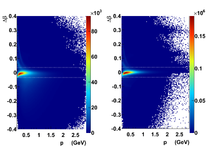
Figure 2: The $\Delta\beta$ distributions for $\pi^{+}$ (left) and $\pi^{-}$ (right). The cut of $-0.035\leq\Delta\beta\leq 0.035$ is shown as the dashed lined in each case.

III.1 Kaon identification

In the reaction of interest, $\gamma p\to K^{0}\Sigma^{*+}(X)\to\pi^{+}\pi^{-}\pi^{+}n(X)$, it is necessary to determine which $\pi^{+}$ comes from the $K^{0}$. It is possible to check both final state $\pi^{+}$’s with the detected $\pi^{-}$ to study the kaon candidates in each case by using the invariant mass.

The invariant mass was selected for each $\pi^{+}\pi^{-}$ pair, as shown in Fig. 3. Whichever $\pi^{+}$ lead to the invariant mass that was closest to the mass of the $K^{0}$ was associated with the $K^{0}$ identification. Afterwards a cut at $\pm 0.01$ GeV about the $K^{0}$ mass was used to clean up the selection. For cases where both $\pi^{+}$ combinations with the $\pi^{-}$ fell within the $K^{0}$ mass limit the wrong $\pi^{+}$ could be selected. Monte Carlo was used to check the frequency of this ambiguity and was found to be $\sim 2\%$ for the $\gamma p\to K^{0}\Sigma^{*+}\to\pi^{+}\pi^{-}\pi^{+}n\pi^{0}$ and $\gamma p\to K^{0}\Sigma^{*+}\to\pi^{+}\pi^{-}\pi^{+}n\gamma$ channels. With additional kinematic constraints these ambiguous events were ultimately rejected.

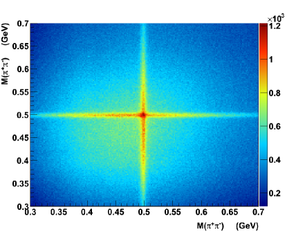
Figure 3: Invariant mass of the $\pi^{+}$-$\pi^{-}$ combination for the two different $\pi^{+}$ detected, prior to any $\pi^{+}$ organization.

III.2 Neutron identification

Neutral particles are detected in CLAS as clusters in the electromagnetic calorimeter (EC) ec not associated with any reconstructed charged track from the drift chambers. The momentum reconstruction depends on the path length and TOF of the neutron. The directional components of the neutral track were found by using the vertex and the cluster position on the EC for that hit. In this experiment the information about the neutral vertex was limited to the information that could be extracted from the other charged particle vertices in the decay chain.

The EC has six triangular sectors made of alternating layers of lead and scintillator. Scintillator layers compose of about 10-cm-wide scintillator strips, where strips in every consecutive layer run parallel to one of the three sides of the triangle. The EC has 13 layers of scintillator strips for each of the three directions making 39 total layers. In each direction the EC is subdivided into an inner stack of 5 layers and an outer stack of 8 layers.

The EC reconstruction software forms a cluster by first identifying a collection of strips in each of the three views. The software requires a set of threshold conditions to be met and that the strips to be contiguous. The groups of strips that pass these conditions define a $peak$ and are organized with respect to the sum of the strip energies. The peak centroid and RMS in each of the three views is obtained and clusters are identified as intersection of centroids of peaks within their RMS. If a given peak contributes to multiple hits, then the energy in each hit due to that peak is calculated as being proportional to the relative sizes of the multiple hits as measured in the other views. For example, if there are multiple hits which have the same U peak, the energy in V and W is added for each of the hits, and the ratio of these summed energies determines the weight of the U peak’s energy of the multiple hits. If the software thresholds for the scintillator strip, peak and weighted hit energy are met then the cluster position and time are recorded. The events EC time (or EC time-of-flight) is defined as the time between the event start time and the time of the EC cluster.

During analysis the strip information was used to determine whether the centroid was reconstructed using only the outer stack of the EC or both the inner stack and outer stack. The centroid could be located in any one of the layers of each stack, however, the cluster reconstruction position did not contain that information, so the hit was assumed to be on the upstream face (closer to the target) of whichever stack the hit was contained in. With the assumed reaction vertex and the EC cluster position, the directional components in $\theta$ and $\phi$ were found, as well as the path length of the neutron. Using the EC time-of-flight the momentum was calculated. The neutrons were differentiated from photons using a $\beta<0.9$ cut.

Neutron detection is essential for the reaction of interest. The neutron momentum was used in combination with the $\pi^{+}$ not associated with the $K^{0}$, to study the kinematics of the $\Sigma^{+}$. Having clean constraints on the $K^{0}$ and $\Sigma^{+}$ is important when considering the event topology $\gamma p\to K^{0}\Sigma^{*+}\to K^{0}\Sigma^{+}(X)$.

A thorough study of the accuracy of the EC for neutron reconstruction in all kinematic ranges has not been achieved previously at CLAS. Obtaining the resolution in all measured variables for neutron reconstruction was an essential part of the present analysis. Correlations between each measured variable in the EC had also not been previously studied. The EC covariance matrix of the neutron can give a lot of information about the quality of the kinematic variables in each region of the EC. These values can then be used to weight the neutron measurements appropriately in kinematic constraints that depend on maximum likelihood methods keller3 .

There are resolution differentials in all measured variables that are related to the acceptance of the EC. Hits from the center of each triangular sector have better measurements over those on the edges due to shower leakage. The inner and outer stacks can act as separate detectors in the sense that if a hit is seen in the outer but not the inner stack, then the inner stack plays no role in the reconstruction of that hit. It is far less common for an event to pass through the inner stack with no effect and to register a hit in the outer stack, but for these events, the outer EC stack was used independently with its own unique resolution parameters for each measured variable. All possible combinations of the measured neutron dependence on $\theta$, $\phi$, and $p$ were studied to develop a complete understanding of the neutron variance and covariance in the EC keller2 .

III.2.1 Neutron detection test

The test reaction $\gamma p\to\pi^{+}\pi^{-}\pi^{+}n$ was isolated in the $g11a$ data set by selecting a $\pi^{-}$ and two $\pi^{+}$, and kinematically fitting to a missing neutron hypothesis and then taking a $10\%$ confidence level cut. Only the detected neutrons found in a direction less than $3^{\circ}$ from the kinematically fit three pion missing momentum were used to ensure the correct neutron. This channel was selected because the final decay products are identical to the reaction of interest $\gamma p\to K^{0}\Sigma^{*+}\to K^{0}\Sigma^{+}(X)$. In addition, the momentum range of the detected particles is the same. Kinematic constraints were imposed to remove possible $\pi^{+}$ $\pi^{-}$ combinations with invariant mass equal to the $K^{0}$, so that only the $\gamma p\to\pi^{+}\pi^{-}\pi^{+}n$ events survived. The simplification made by working with the test channel is that in the $\gamma p\to\pi^{+}\pi^{-}\pi^{+}n$ reaction, there is only one interaction vertex. This implies that the neutron comes from the primary interaction vertex, which can be well determined using the charged pions.

To study the measured neutron variable residuals, we required each event to have one detected neutron and then compared the measured variable with the kinematically fit missing variable in each case. Assuming a high quality missing neutron four vector, this procedure was used to find the change in resolution with respect to all measured variables over the EC face keller2 . Only the events that registered an actual hit in the EC were used to study the resolution. No EC fiducial cuts were applied during the covariance investigation so that the entire EC face could be studied and compared to Monte Carlo. During analysis, only the minimal fiducial cuts were applied of $8^{\circ}<\theta<40^{\circ}$ on the neutron polar angle to maximize the statistics.

For the test channel the neutron vertex was found from a multi-track-vertex fitting procedure to give an accurate vertex (at less than 4% uncertainty in position for the topology of interest) for multiple final state particles all coming from the same vertex mcnabb . Because the neutron came from the primary interaction vertex in this study, its vertex was accurately known. However, for events in which the neutron comes from secondary vertices, its vertex is not as easily obtained. Because the neutron vertex information can affect its reconstructed four momentum, these differences can be important when studying resolutions.

Once the EC neutron covariance matrix for $\gamma p\to\pi^{+}\pi^{-}\pi^{+}n$ was well understood, the Monte Carlo resolution was matched to the data using the same test channel keller2 . The Monte Carlo was then used to study the $\gamma p\to K^{0}\Sigma^{*+}\to K^{0}\Sigma^{+}\pi^{0}$ channel and to find the neutron covariance matrix specific for this topology. In this way the $K^{0}$ interaction point with the beam line could be used as the starting point of the neutron path in the neutron reconstruction process for any of the decays, so no bias was introduced by assuming a $\Sigma^{+}$. This step removed the explicit dependence on the neutron vertex. The Monte Carlo covariance matrix for $\gamma p\to K^{0}\Sigma^{*+}\to K^{0}\Sigma^{+}\pi^{0}$ was then used to tune the data neutron covariance matrix specific to the topology. The change in the momentum resolution from this tuning process was smaller than $5\%$.

In order to obtain a consistent covariance matrix for the neutron, discrimination was made for each neutron between the inner and outer EC stacks in order to calculate the correct path length. In addition, timing and momentum corrections were applied as described below.

III.2.2 Neutron path

As previously stated, the distance that the neutron travels in CLAS was used with the EC time-of-flight to determine the momentum of the neutron. The distance is dependent on the EC stack and the position of the cluster reconstruction. The inner stack cluster reconstruction was always used unless there was only a hit in the outer stack. A determination of whether there was a hit only in the outer stack, the inner stack, or both, was made by checking which EC scintillators were associated with an event. The probability to find a hit in the outer stack alone was less than 15%. For all other neutral hits either the inner stack or both were associated with the hit. If there was a hit only in the outer EC stack, the first layer (layer closest to the target) of the outer stack gave the plane of the EC cluster coordinates. If there was a hit in the inner stack or both, the first layer of the inner stack was used as the plane of the EC cluster coordinates.

III.2.3 Neutron time

The time-of-flight for the neutron came from the difference between the event start time and the EC cluster time. The path length used to reconstruct the neutron momentum, which assumes a hit on the EC face of either the inner or outer stack, was inaccurate by the distance the neutron traveled past the EC face into the detector. A correction was used to compensate for the average additional distance the neutron travels into the EC. In addition the outer stack is farther from the target and for the same event would have a slightly different time response than that of the inner stack.

A correction was implemented directly in the neutron time-of-flight to correct the neutron momentum. This was done by using the calculated neutron time-of-flight and comparing it to the expected time $T_{expected}=L/c\beta_{miss}$. Here, $L$ is the path length of the neutron, and $\beta_{miss}$ is the $\beta$ calculated using the missing momentum and energy of the neutron from the $\gamma p\to\pi^{+}\pi^{-}\pi^{+}(n)$ events that passed a 10% confidence level cut from a kinematic fit under a missing neutron hypothesis. By using $T_{expected}-T_{EC}$ for each stack, a separate correction was found for each case, such that $T_{expected}-(T_{EC}+T_{correction})\sim 0$. By finding separate timing corrections for the inner and outer stacks, the farther distance of the outer stack was compensated for. The separate study of timing corrections for the inner and outer stacks was carried out using the Monte Carlo simulations.

The timing correction used is the same in all directions. However, in order to obtain accurate covariance information an additional momentum correction was required which is sensitive to the geometry of the EC and neutrons trajectory. It was only after all corrections that the residual means of all measured variables were centered around zero to accurately reflect the neutron resolutions.

III.2.4 Neutron momentum correction

A neutron momentum correction was implemented by studying the trend found in momentum and position resolutions over various kinematic ranges. This was done by studying the residuals $\Delta p$, $\Delta\theta$, and $\Delta\phi$ over each variable $p$, $\theta$, and $\phi$. The residual of momentum, $\Delta p$, is defined as the difference between the missing neutron momentum and the reconstructed neutron momentum. Likewise for the directional components $\Delta\theta$ and $\Delta\phi$. The missing neutron four-vector was found by kinematically fitting the charged decay products in the missing mass of the neutron and taking a 10% confidence level cut. In this fit there were three unknowns from the components of the missing momentum vector and four constraints from the conservation of energy and momentum to make a 1-C fit keller3 . The trend of each of the residuals should be distributed around zero, if it is not, the distribution will display a trend that can be used to correct the measured variable. Once the neutron momentum magnitude and directional resolutions are evenly distributed around zero, the missing and detected four-vectors are comparable. This implies that for the majority of events, the detected neutron momentum vector was the same within the experimental resolution as the high quality kinematically fit missing neutron momentum vector.

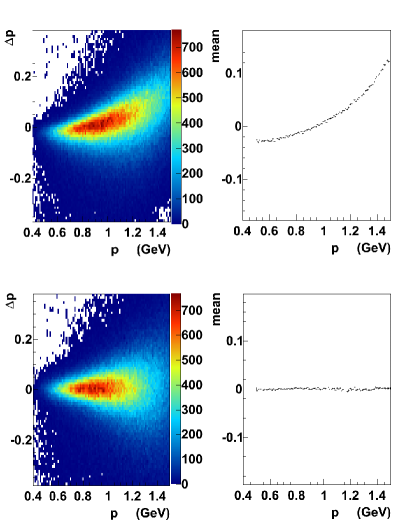
Figure 4: Top left: the neutron $\Delta p$ distribution before correction, top right: the Gaussian mean from the binned fits, bottom left: the corrected distribution, and bottom right: the final corrected Gaussian mean from the binned fits.

Similar corrections were implemented to $\Delta p$ with respect to $\phi$ such that $p^{\prime}=p+f(\phi)$, $\Delta\phi$ with respect to $\phi$ such that $\phi^{\prime}=\phi+f(\phi)$, and $\theta$ with respect to $\theta$ such that $\theta^{\prime}=\theta+f(\theta)$. The Monte Carlo required separate corrections in the same variables that were determined using the same procedures as for the data.

III.2.5 Neutron covariance matrix

The neutron covariance matrix was determined after the corrected neutron path was used with the timing correction implemented for the corresponding EC stack and momentum correction. This covariance matrix was required in order to kinematically fit the neutron with the other detected particles. The variables used to represent the neutron vector components were $\theta$, $\phi$, and $p$, leading to a covariance matrix of

$${\rm\bf V}^{n}_{i}=\left(\begin{matrix}V^{pp}_{i}&V^{p\theta}_{i}&V^{p\phi}_{i}\cr V^{p\theta}_{i}&V^{\theta\theta}_{i}&V^{\phi\theta}_{i}\cr V^{p\phi}_{i}&V^{\phi\theta}_{i}&V^{\phi\phi}_{i}\cr\end{matrix}\right).$$

The variance and correlations of each variable were obtained by studying the differences between the kinematic variables of the detected neutron from the kinematically fit missing neutron. The residuals in each case were sliced and binned to fit with a Gaussian to find the functional dependence in each variable. Once the functional dependence on each variable was found for each $\phi$ and $\theta$ bin, an empirical smearing technique was used to get the Monte Carlo to closely match the same functional dependence seen in the data. Similar steps were taken for the directional components keller2 .

IV Analysis Procedure

In the analysis, progressive steps were taken to remove as much identifiable background as possible while preserving the counts from the channels $\gamma p\to K^{0}\Sigma^{*+}\to K^{0}\Sigma^{+}(\pi^{0})$ and $\gamma p\to K^{0}\Sigma^{*+}\to K^{0}\Sigma^{+}(\gamma)$. The radiative signal was buried by the $\pi^{0}\to\gamma\gamma$ decay and required advanced fitting techniques to resolve the signal. The fitting procedure developed here required that all other backgrounds be removed or extensively minimized to ensure high quality separation between the radiative and strong decays of the $\Sigma^{*+}$.

The goal was then to achieve clean hadron identification before using the fitting procedure for the competing $\pi^{0}$ and radiative signals. For the sake of notation, let $\pi_{1}^{+}$ indicate the $\pi^{+}$ used in the $K^{0}$ invariant mass selection, such that $\pi_{1}^{+}$ is the $\pi^{+}$ that forms the closest known $K^{0}$ mass when combined with the $\pi^{-}$. Naturally $\pi_{2}^{+}$ is the other detected $\pi^{+}$. Fig. 5 shows the invariant mass of the $\pi_{1}^{+}$-$\pi^{-}$ (upper left), missing mass off the $\pi_{1}^{+}$-$\pi^{-}$ (upper right), the n-$\pi_{2}^{+}$ invariant mass (lower left), and the missing mass squared of all the detected particles (lower right). The distributions in Fig. 5 are before any kinematic constraints and after the $\pi^{+}$ assignments are made. The $K^{0}$ was cut about $\pm 0.01$ GeV of the known $K^{0}$ mass to reduce the $\pi^{+}$-$\pi^{-}$ background. Fig. 6 shows the invariant mass of the n-$\pi_{2}^{+}$ (dashed lines show the cut that was implemented) (upper left), missing mass off the $K^{0}$ (upper right), the missing energy off all detected particles (dashed lines show the cut that was implemented) (lower left), and the missing mass squared of all the detected particles (lower right), after the $K^{0}$ cut. The $\Sigma^{+}$ peak is clearly visible as seen in the (upper left) plot. The clear visible peak in the missing mass squared at the $\pi^{0}$ mass is also an indication that the neutron measurement is effective.

A Monte Carlo study on the phase space of the $\gamma p\to K^{0}\Sigma^{*+}\to K^{0}\Sigma^{+}(X)$ reaction indicated that most events from the missing energy boosted in the $\Sigma^{*+}$ frame $E_{x}$ should be in the range of 0-0.25 GeV. A cut at 0.24 GeV was chosen to clean up the $\Sigma^{*+}$ candidates. This cut preserved $\sim 80\%$ of the radiative and $\pi^{0}$ signals, while substantially reducing the background under the $\Sigma^{*+}$. Fig. 7 shows an example of the Monte Carlo missing energy distribution for the $\gamma p\to K^{0}\Sigma^{*+}\to K^{0}\Sigma^{+}\gamma$ reaction with the dotted line indicating the 0.24 GeV cut. Fig. 8 shows the results on the missing mass off the $K^{0}$. A cut on the invariant mass of the n-$\pi_{2}^{+}$ combination along with the missing energy cut cleans up the excited-state hyperon spectrum, making the $\Sigma^{*+}$ quite prominent. Finally a $\pm 0.03$ GeV cut was applied to the missing mass off the $K^{0}$ around the known mass of the $\Sigma^{*+}$.

Fig. 9 shows the missing mass squared of all detected particles after all of the mentioned cuts. A clear $\pi^{0}$ peak is present with some smaller but unknown amount of radiative signal at zero missing mass. Fig. 10 shows the the missing mass off the n-$\pi_{2}^{+}$ combination. The missing mass off the $\Sigma^{+}$ will be used in the background analysis.

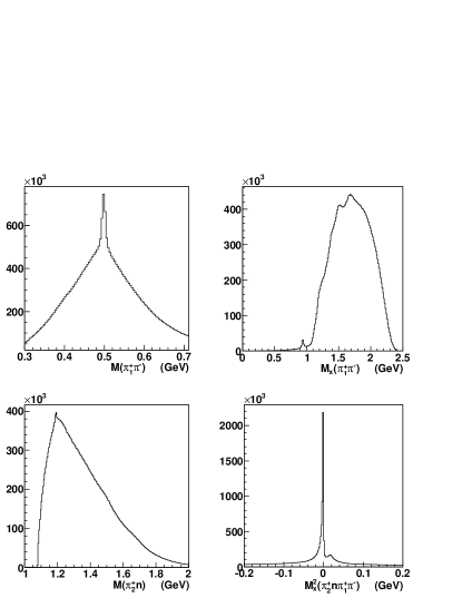
Figure 5: The invariant mass of the $\pi_{1}^{+}$-$\pi^{-}$ (upper left), the missing mass off the $\pi_{1}^{+}$-$\pi^{-}$ (upper right), the n-$\pi_{2}^{+}$ invariant mass (lower left), and the missing mass squared of all the detected particles (lower right). All distributions are before any kinematic constraints.

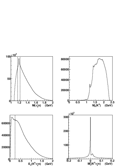
Figure 6: The invariant mass of the n-$\pi_{2}^{+}$ with the dotted lines showing the $|M(\pi_{2}^{+}n)-M_{\Sigma^{+}}|<0.01$ GeV cut (upper left), the missing mass off the $K^{0}$ (upper right), the total missing energy with the dotted line showing the cut used (lower left), and the missing mass squared of all the detected particles (lower right) after the $\pm 0.01$ GeV cut on the $K^{0}$ peak.

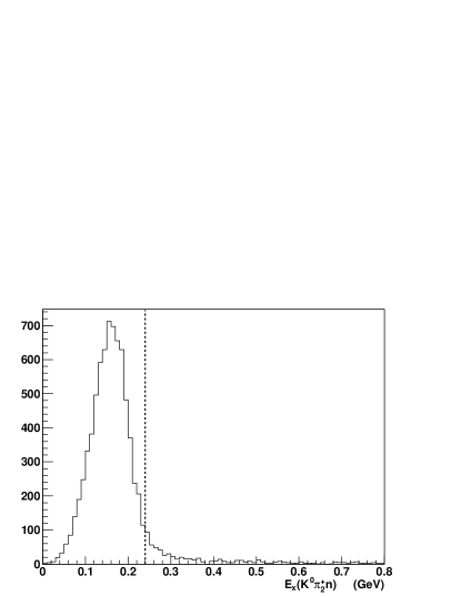
Figure 7: The Monte Carlo missing energy distribution for the $\gamma p\to K^{0}\Sigma^{*+}\to K^{0}\Sigma^{+}\gamma$ reaction with the dotted line indicating the 0.24 GeV cut.

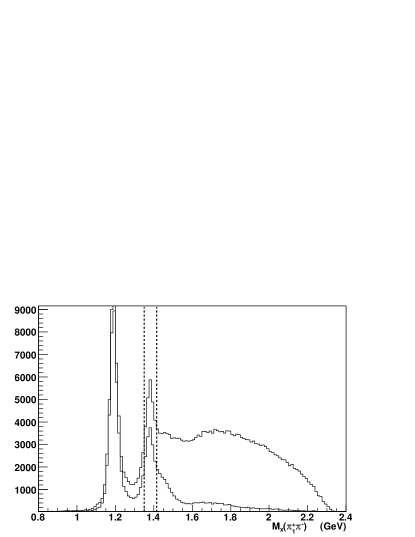
Figure 8: The missing mass off the $\pi_{1}^{+}$-$\pi^{-}$ with three progressive cuts applied to isolate the $\Sigma^{*+}$ events. First $|M(\pi_{2}^{+}n)-M_{\Sigma^{+}}|<0.01$ GeV, next shown are the events left over after the $E_{x}<0.24$ GeV cut, and finally the dotted lines show the $\pm$0.03 GeV cut around the mass of the $\Sigma^{*+}$.

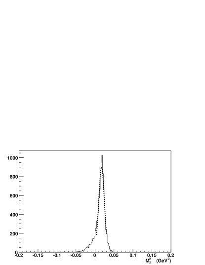
Figure 9: The missing mass squared of all detected particles after all analysis cuts. A Gaussian fit gives a mean of 0.018$\pm$0.0002 GeV.

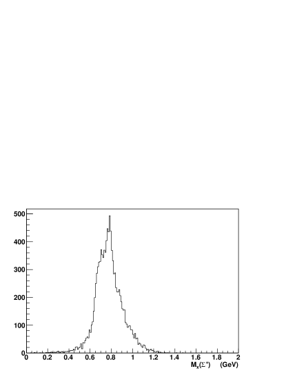
Figure 10: The missing mass of the $\Sigma^{+}$.

IV.1 Simulations

A Monte Carlo simulation of the CLAS detector was performed using GEANT geant , set up for the $g11a$ run conditions. The experimental photon energy distribution for an incident electron beam of 4.0186 GeV was used to determine the energies of the incident photons in the simulation. Events were generated for the radiative channel ($\Sigma^{+}(1385)\rightarrow\Sigma^{+}\gamma$), the normalization reaction ($\Sigma^{+}(1385)\rightarrow\Sigma^{+}\pi^{0}$), and several background reactions.

A phase space event generator was used with a variable $t$-dependence such that a channel with a $K^{0}$ was generated uniformly in the center-of-mass frame in $\phi$ with a $t$-dependent distribution in $\theta_{cm}$ according to $P(t)\propto e^{bt}$ with $b$=2.0 GeV^-2. Gaussian distributions in $x$ and $y$ with $\sigma=0.5$ cm were used to approximate the beam width at the target. Events were generated uniformly along the length of the target. These generated events were fed into a simulation of the CLAS detector.

For each contributing channel the differential cross section was found using data to weight the strength and angular distribution in the Monte Carlo generator. A very careful empirical smearing procedure was used to match the Monte Carlo and data resolutions. This procedure is discussed in Refs. keller3 and keller2 . Ultimately the missing mass squared from Monte Carlo, $M_{x}^{2}(K^{0}\Sigma^{+})$, gave very good agreement with the shape of the experimental data as shown in Fig. 9.

This analysis relies on an understanding of the contributing leakage of background channels into the $\pi^{0}$ and radiative signal peaks. For example, $\pi^{0}$ leakage from a background channel such as $\gamma p\to\omega\Delta^{+}\to\pi^{+}\pi^{-}\pi^{0}n\pi^{+}$ will lead to over-counting of $\Sigma^{*+}\to\Sigma^{+}\pi^{0}$ events. The Monte Carlo of various possible contributions was used to study the possible background leakage at various stages of the analysis. The acceptances of each possible background were used to study the possible effect on the final reported ratio.

At this stage of the analysis the most likely background reaction is $\gamma p\to\omega\Delta^{+}$, followed by $\Delta^{+}\to n\pi^{+}$ decay. The $\omega$ decays primarily to $\pi^{+}\pi^{-}\pi^{0}$ followed by $\pi^{0}\to 2\gamma$. The full reaction $\gamma p\to\omega\Delta^{+}$ then has the same final state as $K^{0}\Sigma^{*+}\to\Sigma^{+}\pi^{0}$ and must be carefully considered. This is also true for reactions like $\gamma p\to\omega N^{*}$. The $N(1440)$ has a relatively large decay width at 250-450 MeV pdg , which implies possible leakage into any cut around the $\Sigma^{*+}$. This is the reason for the extra steps to isolate the $\Sigma^{*+}$ as shown in Fig. 8. Due to the constraints on the $\pi^{+}$ and $n$, along with the series of cuts shown in Fig. 8, the leakage from the $N^{*}$ decay was negligible. However, because the $\Delta^{+}$ is very close in mass to the $\Sigma^{+}$ and the $\pi^{+}\pi^{-}$ from the $\omega$ decay has a similar phase space to the $K^{0}$, there was some $\gamma p\to\omega\Delta^{+}$ leakage that needed to be accounted for.

The contribution of the $K^{*0}$ background was also studied. The constraints on the reconstructed $K^{0}$, combined with the missing mass constraint off the $K^{0}$ to be the mass of the $\Sigma^{*+}$, should minimize any $K^{*0}$ contribution. However, because the reaction $\gamma p\to K^{*0}\Sigma^{+}$ has the same possible final states that are being analyzed, it was carefully considered. The Monte Carlo investigation indicated that there were contributions that needed to be accounted for.

Also investigated with Monte Carlo was the reaction $\gamma p\to m^{*}N^{*}$, where $m^{*}$ is any meson that can decay to $\rho\pi^{0}$, and the $N^{*}\to N\pi^{+}$ provides the detected pion. Similarly, $\gamma p\to\rho N^{*}$, where the $N^{*}$ decay to $n\pi^{+}\pi^{0}$ was a possible contaminant. In addition to the kinematic constraints previously mentioned, these backgrounds cannot contribute for low $W$ ($W<1.6$ GeV). For testing purposes of these types of reactions, the channel $\rho N(1520)$ was considered. The $\rho(770)$ has a width of $\Gamma=150.3$ MeV and decays almost 100% to $\pi\pi$, so it was possible to leak under the $K^{0}$ invariant mass cut. Ultimately all contributions of the channel type $\gamma p\to m^{*}N^{*}$ were found to be negligible (zero acceptance).

Based on the possible final state decay products, the reactions $\gamma p\to\eta n\pi^{+}$, $\gamma p\to K^{0}\Sigma^{0}\pi^{+}$, and $\gamma p\to K^{0}\Sigma^{+}$ were also considered. These backgrounds also have negligible acceptance as determined from high-statistics Monte Carlo studies using the same event selection as for the data, and hence were dismissed.

IV.1.1 Minimization of the $\omega$ and $K^{*0}$ backgrounds

As indicated in the previous section, the $\gamma p\to\omega\Delta^{+}$ and $\gamma p\to K^{*0}\Sigma^{+}$ channels are the most likely background contributors. The branching ratio of $\omega\to\pi^{+}\pi^{-}\pi^{0}$ is $89.2\pm 0.7\%$ pdg , implying a high probability of overlap with the normalization channel $\gamma p\to K^{0}\Sigma^{*+}\to\pi^{+}\pi^{-}\pi^{+}n(\pi^{0})$. The $\gamma p\to K^{*0}\Sigma^{+}$ channel was a concern for the same reason. To get an indication of how much these channels were present in the data, the missing mass off the $\pi_{2}^{+}$-$n$ combination was used. For the $\gamma p\to\omega\Delta^{+}$ ($\gamma p\to K^{*0}\Sigma^{+}$) channel the missing mass off $\pi_{2}^{+}$-$n$ should show a $\omega$ ($K^{*0}$) peak. The missing mass spectrum off the $\pi_{2}^{+}$-$n$ combination from the Monte Carlo of the $\gamma p\to K^{0}\Sigma^{*+}\to\pi^{+}\pi^{-}\pi^{+}n(\pi^{0})$ channel was compared to the same distribution from data. To isolate the $\pi^{0}$ channel in the data, a kinematic fit to the missing $\pi^{0}$ with a $10\%$ confidence level cut was applied to leave only the final state $\pi^{+}\pi^{-}\pi^{+}n\pi^{0}$ in the data. A direct comparison between the data and Monte Carlo of the missing mass spectrum off the $\pi_{2}^{+}$-$n$ combination then deviated where background was present (normalizing the Monte Carlo to the data). It is clear from the comparison shown in Fig. 11 that there is a non-negligible amount of $\omega$ events. The number of events with a $K^{*0}$ present is too small to be visible.

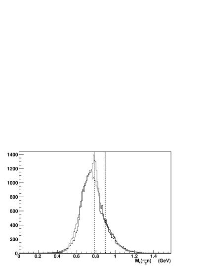
Figure 11: The Monte Carlo and data distributions for the missing mass off the $\pi_{2}^{+}n$ combination with the data showing a $\omega$ peak. The Monte Carlo shown is for the reaction $\gamma p\to K^{0}\Sigma^{*+}\to\pi^{+}\pi^{-}\pi^{+}n\pi^{0}$, indicating the expected missing mass off the $\pi_{2}^{+}n$ combination if no background was present. The dashed lines indicate the known masses of the $\omega$ and $K^{*0}$.

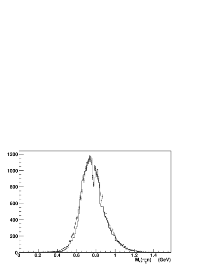
Figure 12: The Monte Carlo (lines) and data (points) distributions for the missing mass off the $\pi_{2}^{+}n$ combination (as shown in Fig. 11) after the $P(\chi^{2})<1\%$ cut showing that the distributions now match in the $\omega$ mass region.

To remove the majority of the $\omega$ events a kinematic fit was performed with a missing $\pi^{0}$ hypothesis, while constraining the $\pi_{1}^{+},\pi^{-}$ and $(\pi^{0})$ to have the $\omega$ mass, resulting in a 2-C fit. High confidence level candidates were then rejected as part of the identifiable $\omega$ background. Various confidence level cuts were tested until the data matched the Monte Carlo in the mass range of the $\omega$ (within the statistical error bars of the data). Ultimately a confidence level cut of $P(\chi^{2})<1\%$ was used, resulting in the comparison seen in Fig. 12. The same cut was used to reduce the possible $\gamma p\to\omega\Delta^{+}\to\pi^{+}\pi^{-}\pi^{+}n(\gamma)$ background by imposing the constraint on the $\pi_{1}^{+},\pi^{-}$ and $(\gamma)$ to be $\omega$. In this case it was not possible to use the Monte Carlo and data to check in the same way, and so a $P(\chi^{2})<1\%$ cut was used. The same cut was also used under a $K^{*0}$ hypothesis to reduce the acceptance of the $\gamma p\to K^{*0}\Sigma^{+}\to\pi^{+}\pi^{-}\pi^{+}n(\pi^{0})$ channel. Similarly for the $\gamma p\to K^{*0}\Sigma^{+}\to\pi^{+}\pi^{-}\pi^{+}n(\gamma)$ with the hypothesis of the $\pi_{1}^{+},\pi^{-}$ and $(\gamma)$ to be $K^{*0}$.

Even with the above cuts in place, a small amount of the $\omega$ and $K^{*0}$ background still slipped through. An estimate of this leakage was found and then subtracted out of the final result, as discussed in the following sections.

IV.1.2 Cross sections

To tune the $\Sigma^{*+}$ Monte Carlo, the differential cross sections for the reactions $\gamma p\to K^{0}\Sigma^{*+}\to\pi^{+}\pi^{-}n\pi^{+}\pi^{0}$, $\gamma p\to K^{*0}\Sigma^{+}\to\pi^{+}\pi^{-}\pi^{0}n\pi^{+}$, and $\gamma p\to\omega\Delta^{+}\to\pi^{+}\pi^{-}\pi^{0}n\pi^{+}$ were obtained. The shapes of the differential cross sections were then used to adjust the event generators. In each case a $1/E_{\gamma}$ photon energy distribution was used in the generator.

A normalization procedure shown to accurately reproduce a number of well-measured channels was used for each cross section mccracken . The following is a discussion of the procedure used to extract the $\gamma p\to K^{0}\Sigma^{*+}$ cross section. A similar procedure was followed for the two background channels.

With all of the aforementioned constraints the $\gamma p\to K^{0}\Sigma^{*+}\to K^{0}\Sigma^{+}\pi^{0}$ reaction was easily isolated with a kinematic fit to the missing $\pi^{0}$. A $10\%$ confidence level cut was applied to ensure channel purity. The yield was determined by the ratio of the raw $\Sigma^{+}\pi^{0}$ events to the number of incident photons in each $E_{\gamma}$ bin, so as to normalize with the bremsstrahlung spectrum. Corrections were made for each bin with the newly obtained acceptances. The angular dependence in the generator was initially flat with a zero $t$-slope dependence. After the differential cross section was obtained, the distributions were used to adjust the $\Sigma^{*+}$ generator. Each corresponding angle and energy bin was filled according to the distributions seen in the data results. Each angle bin was divided into $E_{\gamma}$ bins and represented accordingly in the new event weighting scheme of the generator. The adjusted generator was then used to produce new Monte Carlo and obtain more accurate acceptances. This process was then iterated until no change was seen to the differential cross sections within the statistical uncertainties. After these modifications were made, the resulting Monte Carlo was compared with the data, using the momentum distributions for the $\pi^{-}$, $\pi^{+}$, and neutron tracks, as well as the $K^{0}$ lab frame angle distribution, and found to closely match the data within the statistical uncertainties, see Fig. 13.

The same corrections were applied to the $\gamma p\to K^{0}\Sigma^{*+}\to K^{0}\Sigma^{+}\gamma$ cross sections. The nature of the corrections to the Monte Carlo were specific to the $\gamma p\to K^{0}\Sigma^{*+}$ cross section and so the corrections could be applied without discrimination between the electromagnetic and strong decays of the baryon.

To calculate the acceptance of the signal and background reactions, an extraction method used to resolve the radiative and $\pi^{0}$ channels was required and will be discussed next.

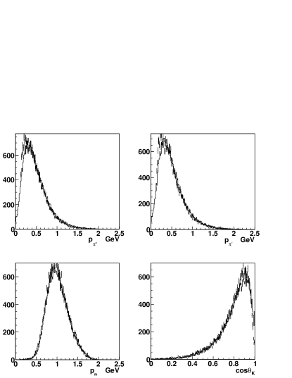
Figure 13: The momentum distributions for the $\pi^{+}$, $\pi^{-}$, and neutron are shown in the first 3 panels, with the cosine of the kaon lab frame angular distribution in the last panel, for the reaction $\gamma p\to K^{0}\Sigma^{*+}\to\pi^{-}\pi^{+}n\pi^{+}\pi^{0}$. The data and Monte Carlo are shown as the histogram and points, respectively, which closely overlap.

IV.2 Fitting technique

The two-step kinematic fitting procedure developed in Ref. kellpaper was employed to resolve the radiative and strong decay signals. Because of such similar topologies and the small relative size of the radiative signal, the kinematic fitting procedure could not be expected to cleanly separate the $\Sigma^{+}\gamma$ events from the overwhelming $\Sigma^{+}\pi^{0}$ events in a single fit. Thus we employed a two-step kinematic fitting procedure, making first a kinematic fit to a missing $\pi^{0}$ hypothesis, then checking the quality of the fit of the low confidence level candidates in a second kinematic fit to the actual radiative hypothesis.

In order to check the quality of the kinematic fit to a particular hypothesis, we studied the $\chi^{2}$ distribution from the fitting results. In this procedure all detected particles were kinematically fit to the appropriate missing mass hypothesis. An additional constraint was introduced into the kinematic fitting enabling analysis of the more well-behaved 2-C $\chi^{2}$ distribution, as opposed to the 1-C distribution, to test the quality of the candidates with the hypothesis used. The constraint required that the neutron and $\pi^{+}$ track have an invariant mass of the $\Sigma^{+}$ in the hypothesis. The detected particle tracks were kinematically fit as the final stage of analysis and filtered with the confidence level cut. In this fit there were three unknowns ($\vec{p}_{x}$) and five constraint equations, four from conservation of momentum and then the additional invariant mass condition. This makes a 2-C kinematic fit. In the attempt to separate the various contributions of the $\Sigma^{*+}$ radiative decay and the decay to $\Sigma^{+}\pi^{0}$, the events were fit using different hypotheses for the topology:

	$\gamma p\rightarrow\pi^{+}\pi^{-}\pi^{+}n(\pi^{0})$	2-C
	$\gamma p\rightarrow\pi^{+}\pi^{-}\pi^{+}n(\gamma)$	2-C.

The constraint equations were

$$\left[\begin{array}[]{c}(E_{\pi^{+}_{2}}+E_{n})^{2}-(\vec{p}_{\pi^{+}_{2}}+\vec{p}_{n})^{2}-M^{2}_{\Sigma^{+}}\\ E_{beam}+M_{p}-E_{\pi^{+}}-E_{\pi^{-}}-E_{\pi^{+}}-E_{n}-E_{x}\\ \vec{p}_{beam}-\vec{p}_{\pi^{+}}-\vec{p}_{\pi^{-}}-\vec{p}_{\pi^{+}}-\vec{p}_{x}\end{array}\right]=\vec{0}.$$ (5)

$\vec{p}_{x}$ and $E_{x}$ represent the missing momentum and energy of the undetected $\pi^{0}$ or $\gamma$.

Then a fit function was made for a 2-C $\chi^{2}$ distribution following from Ref. keller3 as

$$f(\chi^{2})=\frac{P_{0}}{2}e^{-P_{1}\chi^{2}/2}+P_{2}.$$ (6)

This fit function has a flat background term, $P_{2}$. $P_{1}$ was used to measure how close the distribution in the histogram was to the ideal theoretical $\chi^{2}$ distribution for two degrees of freedom.

Because there were two kinematic fits for both the $\pi^{0}$ and radiative channels, some new notation is introduced. The first confidence level cut used to filter out the larger $\pi^{0}$ signal from the radiative signal by using a kinematic fit to $\Sigma^{+}(\pi^{0})$ and taking only the low confidence level candidates is denoted as $P_{\pi}^{a}(\chi^{2})$. The final kinematic fit used to isolate the radiative signal, using a $\Sigma^{+}(\gamma)$ hypothesis has a confidence level cut denoted as $P_{\gamma}^{b}(\chi^{2})$, taking only the high confidence level candidates. Optimization studies have been previously done to constrain the choice of $P_{\pi}^{a}(\chi^{2})$ and $P_{\gamma}^{b}(\chi^{2})$ keller3 .

IV.3 Ratio calculation

The $\pi^{0}$ leakage into the $\gamma$ channel was the dominant correction to the radiative branching ratio. To properly calculate the ratio, the leakage into the $\pi^{0}$ region from the $\gamma$ channel was also used. Taking just these two channels into consideration, the number of $true$ counts is represented as $N(\Sigma\gamma)$ for the $\Sigma^{*+}\to\Sigma^{+}\gamma$ channel and $N(\Sigma\pi)$ for the $\Sigma^{*+}\to\Sigma^{+}\pi^{0}$ channel. The acceptance under the $\Sigma^{*+}\to\Sigma^{+}\gamma$ hypothesis is written as $A_{\gamma}(X)$, with the subscript showing the hypothesis type and the actual channel of Monte Carlo input that was used to obtain the acceptance value indicated in the parentheses. For the calculated acceptance of the $\Sigma^{*+}\to\Sigma^{+}\gamma$ channel under the $\Sigma^{*+}\to\Sigma^{+}\gamma$ hypothesis, the acceptance is $A_{\gamma}(\Sigma\gamma)$, and for the $\Sigma^{*+}\to\Sigma^{+}\pi^{0}$ hypothesis it is $A_{\pi}(\Sigma\gamma)$. It is now possible to express the measured yields for each channel $n_{\gamma}$ and $n_{\pi}$ as

$$n_{\gamma}=A_{\gamma}(\Sigma\gamma)N(\Sigma\gamma)+A_{\gamma}(\Sigma\pi)N(\Sigma\pi)$$ (7)

$$n_{\pi}=A_{\pi}(\Sigma\pi)N(\Sigma\pi)+A_{\pi}(\Sigma\gamma)N(\Sigma\gamma).$$ (8)

The desired branching ratio of the radiative channel to the $\pi^{0}$ channel using the $true$ counts is then $R=N(\Sigma\gamma)/N(\Sigma\pi)$. Solving for $R$ to get the branching ratio expressed in terms of measured values and acceptances gives

$$R=\frac{n_{\gamma}A_{\pi}(\Sigma\pi)-n_{\pi}A_{\gamma}(\Sigma\pi)}{n_{\pi}A_{\gamma}(\Sigma\gamma)-n_{\gamma}A_{\pi}(\Sigma\gamma)}.$$ (9)

Equation 9 is based on the assumption that there are no further background contributions. The formula for the branching ratio to take into account background from the $\omega\Delta^{+}$ channel, as an example, can be expressed as

$$R = {\Delta n_{\gamma}A_{\pi}(\Sigma\pi)-\Delta n_{\pi}A_{\gamma}(\Sigma\pi)\over\Delta n_{\pi}A_{\gamma}(\Sigma\gamma)-\Delta n_{\gamma}A_{\pi}(\Sigma\gamma)},$$

where

$$\Delta n_{\pi} = n_{\pi}-N_{\pi}(\omega\rightarrow\pi^{+}\pi^{-}\pi^{0})$$ (11)

$$- N_{\pi}(\omega\rightarrow\pi^{+}\pi^{-}\gamma)$$

and

$$\Delta n_{\gamma} = n_{\gamma}-N_{\gamma}(\omega\rightarrow\pi^{+}\pi^{-}\gamma)$$ (12)

$$- N_{\gamma}(\omega\rightarrow\pi^{+}\pi^{-}\pi^{0}).$$

The $n_{\gamma}$ ($n_{\pi}$) terms come directly from the yield of the kinematic fits and represent the measured number of photon (pion) candidates. In the notation used, lowercase $n$ represents the measured counts, while uppercase $N$ represents the acceptance corrected or derived quantities. The $N_{\gamma,\pi}$ terms are corrections needed for the leakage from the $\omega\Delta^{+}$ channel (an arbitrary number of background types $N_{\gamma,\pi}(X)$ can be accounted for in this manner). The notation utilized is such that the pion (photon) contributions are denoted $N_{\pi}$ ($N_{\gamma}$), so that $N_{\gamma}(X)$ denotes the relative leakage of the $(X)$ channel under the $\Sigma^{+}\gamma$ hypothesis and $N_{\pi}(X)$ denotes the relative leakage of the $X$ channel under the $\Sigma^{+}\pi^{0}$ hypothesis.

The final acceptance for each channel was determined after the final set of confidence level cuts was taken. After the background acceptances were minimized, an estimate of the background contributions was found for each relevant case.

V Signal Extraction

Each Monte Carlo channel was run through the analysis with the same cuts as used for the data. These cuts for the extraction of the radiative and $\pi^{0}$ signals are listed in Table 1. The cuts are listed in the order implemented. The first cut, (1), was on the $K^{0}$ mass and restricted the $\pi^{+}_{1},\pi^{-}$ sample. The second cut, (2), on the $\Sigma^{+}$ mass was implemented to clean up the $\pi_{2}^{+},n$ sample prior to the more restrictive cuts, (5)-(8). The missing energy restriction used to reduce background is number (3). Cut (4) restricted the missing mass off the $K^{0}$ to be in the range of the $\Sigma^{*+}$. Cuts (5) and (6) list the final confidence level cuts used from the kinematic fit to isolate the missing $\pi^{0}$. Cuts (7) and (8) were used to isolate the radiative decay. The second column lists whether the cut was applied to just one channel or both.

Table 1: The cuts used to extract the final radiative and $\pi^{0}$ counts. (See text for details.)

Cut Used	(Applied)
(1) $|M(\pi_{1}^{+}\pi^{-})-M_{K^{0}}|<0.01$ GeV	($both$)
(2) $|M(\pi_{2}^{+}n)-M_{\Sigma^{+}}|<0.01$ GeV	($both$)
(3) $E_{x}<0.24$ GeV	($both$)
(4) $|M_{x}(\pi_{1}^{+}\pi^{-})-M_{\Sigma^{*+}}|<0.03$ GeV	($both$)
(5) $P^{a}_{\gamma}(\chi^{2})<0.01\%$	($\pi^{0}$)
(6) $P^{b}_{\pi}(\chi^{2})>10\%$	($\pi^{0}$)
(7) $P^{a}_{\pi}(\chi^{2})<0.01\%$	($\gamma$)
(8) $P^{b}_{\gamma}(\chi^{2})>10\%$	($\gamma$)

The two-step kinematic fitting procedure was used to isolate the radiative signal from the $\pi^{0}$ channel. In this procedure two separate kinematic fits were performed, one with zero missing mass for the $\gamma$ and the other with the missing mass of the $\pi^{0}$. The fit function in Eq. 6 was used to fit the $\chi^{2}$ distributions to determine the resulting quality of candidates present in the fit. The parameter $P_{1}$ was used to measure how close the distribution in the histogram was to the $ideal$ theoretical $\chi^{2}$ distribution for two degrees of freedom. The pure radiative decay Monte Carlo was used to determine the value of the expected $P_{1}$ parameter. Fig. 14 (A) shows the $\chi^{2}$ distribution for a kinematic fit of the Monte Carlo channel $\gamma p\to K^{0}\Sigma^{*+}\to\pi^{+}\pi^{-}\pi^{+}n\pi^{0}$ under the radiative hypothesis, displaying a highly distorted $\chi^{2}$ distribution. Fig. 14 (B) shows the $\chi^{2}$ distribution from the same kinematic fit under a radiative hypothesis of the Monte Carlo channel $\gamma p\to K^{0}\Sigma^{*+}\to\pi^{+}\pi^{-}\pi^{+}n\gamma$, a fit using Eq. 6 after all the kinematic cuts up to (4) in Table 1. The parameter $P_{1}$ was used as the $ideal$ value to expect. After obtaining the expected $P_{1}$, a kinematic fit to the data was performed using both hypotheses.

The first confidence level cut $P_{\pi}^{a}(\chi^{2})$ was used to filter out the larger $\pi^{0}$ signal from the radiative signal by using a kinematic fit to a $\Sigma^{+}(\pi^{0})$ hypothesis and taking only the low confidence level candidates. This confidence level cut was checked and made more restrictive until $P_{1}$ from the data matched the expected value from Monte Carlo (within the projected error bars). Fig. 14 (C) shows the $\chi^{2}$ distribution and fit before any $P_{\pi}^{a}(\chi^{2})$ cut was applied and Fig. 14 (D) shows the distribution after a $P_{\pi}^{a}(\chi^{2})<0.01\%$ cut was applied. The final confidence level cut $P_{\gamma}^{b}(\chi^{2})$ from the kinematic fit to a $\Sigma^{+}(\gamma)$ hypothesis was used on the remaining candidates. Only the high confidence level candidates were preserved.

Note that the yields for the $\Sigma^{+}\pi^{0}$ decay will be reduced for a lower value of $P_{\pi}^{a}(\chi^{2})$, which is desirable for extracting the radiative decay signal. On the other hand, this cut cannot be made arbitrarily small, since it reduces the statistics ($i.e.$, increases the statistical uncertainty). Similarly, the $\Sigma^{+}\gamma$ signal will be purified by a higher cut on $P_{\gamma}^{b}(\chi^{2})$, but again the higher the cut, the lower the statistics. The Monte Carlo was used to examine the acceptance of these cuts for various branching ratios ($\Sigma^{+}\gamma/\Sigma^{+}\pi^{0}$), which is discussed in the next section. Ultimately, the branching ratio extracted from the data should not depend on the cut points chosen (assuming the Monte Carlo gives accurate cut acceptances). The Monte Carlo was then used to optimize the trade-off between statistical uncertainty and systematic uncertainty (due to the choice of confidence level cuts based on a more quantitative analysis of $P_{1}$). The cut value of $P^{a}(\chi^{2})<0.01\%$ showed consistent optimization with $P^{b}(\chi^{2})>10\%$ for this topology and range of statistics as listed in Table 1. Details of the optimization method of the confidence level cuts using the Monte Carlo are described in Ref. keller3 . The confidence level distribution under the radiative hypothesis before and after the $P^{a}_{\pi}(\chi^{2})<0.01\%$ cut is shown in Fig. 15(A). Likewise, the confidence level distribution for a fit to the data under the missing $\pi^{0}$ hypothesis before and after the $P^{a}_{\gamma}(\chi^{2})<0.01\%$ cut is shown in Fig. 15(B).

The same cuts determined to effectively isolate the radiative signal, $P^{a}_{\pi}(\chi^{2})<0.01\%$ with $P^{b}_{\gamma}(\chi^{2})>10\%$, were used to isolate the $\pi^{0}$ channel used for normalization of the ratio, such that $P^{a}_{\gamma}(\chi^{2})<0.01\%$ is used with $P^{b}_{\pi}(\chi^{2})>10\%$. This can be denoted as $P^{a}_{\pi}(\chi^{2})=P^{a}_{\gamma}(\chi^{2})<0.01\%$ and $P^{b}_{\gamma}(\chi^{2})=P^{b}_{\pi}(\chi^{2})>10\%$. The final missing mass squared distribution after all cuts is shown in Fig. 16 before the two sets of confidence level cuts and after.

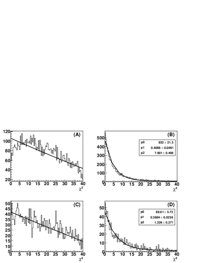
Figure 14: Plot (A) shows the $\chi^{2}$ distribution for the Monte Carlo channel $\gamma p\to K^{0}\Sigma^{*+}\to\pi^{+}\pi^{-}\pi^{+}n\pi^{0}$ under the radiative hypothesis, displaying a highly distorted $\chi^{2}$ distribution. Plot (B) shows the fit results for $\gamma p\to K^{0}\Sigma^{*+}\to\pi^{+}\pi^{-}\pi^{+}n\gamma$, displaying a reasonable $\chi^{2}$ distribution with the $ideal$ $P_{1}$. The radiative hypothesis kinematic fit $\chi^{2}$ distribution and distribution fit to data before any $P_{\pi}^{a}(\chi^{2})$ cut is applied is shown in (C) and the same distribution after a $P_{\pi}^{a}(\chi^{2})<0.01\%$ cut is applied is shown in (D).

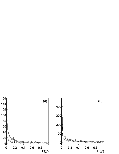
Figure 15: (A) The confidence level distribution for a fit to the data under the radiative hypothesis before the $P^{a}_{\pi}(\chi^{2})<0.01\%$ cut (line) and after (dotted line). (B) The confidence level distribution for a fit to the data under the missing $\pi^{0}$ hypothesis before the $P^{a}_{\gamma}(\chi^{2})<0.01\%$ cut (line) and after (dotted line).

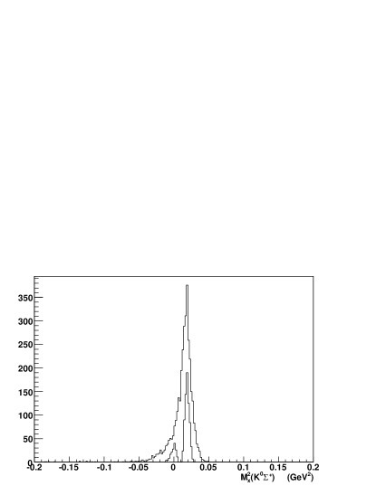
Figure 16: The missing mass off of all detected particles. The plot shows the final radiative candidates at zero missing mass after the $P^{a}_{\pi}(\chi^{2})<0.01\%$ and $P^{b}_{\gamma}(\chi^{2})>10\%$ cuts. Also shown are the final $\pi^{0}$ candidates after the $P^{a}_{\gamma}(\chi^{2})<0.01\%$ and $P^{b}_{\pi}(\chi^{2})>10\%$ cuts.

The acceptances were found for each contributing channel and are listed in Table 2. Each of the channels in Table 2 was generated with enough statistics so that the statistical uncertainty would not contribute in the final ratio calculation. The value of the acceptance for the $\pi^{0}$ ($\gamma$) hypothesis is listed under the $A_{\pi}$ ($A_{\gamma}$) column. The uncertainty is statistical only.

Table 2: Acceptances (in units of $10^{-3}$) for the channels that survive all cuts. All of the cuts used to obtain the acceptance values are listed in Table 1. The uncertainties are statistical only. The two columns contain the acceptance for each hypothesis $A_{\pi}$, $A_{\gamma}$.

Reaction	$A_{\pi}$	$A_{\gamma}$
$K^{0}\Sigma^{*+}\rightarrow K^{0}\Sigma^{+}\gamma$	0.0644$\pm$0.0040	0.6244$\pm$0.0125
$K^{0}\Sigma^{*+}\rightarrow K^{0}\Sigma^{+}\pi^{0}$	0.6502$\pm$0.0128	0.0591$\pm$0.0038
$K^{*0}\Sigma^{+}\rightarrow K^{0}\Sigma^{+}\gamma$	0.0018$\pm$0.0005	0.0186$\pm$0.0021
$K^{*0}\Sigma^{+}\rightarrow K^{0}\Sigma^{+}\pi^{0}$	0.0231$\pm$0.0023	0.0050$\pm$0.0011
$\omega\Delta^{+}\rightarrow\pi^{+}\pi^{-}\pi^{0}n\pi^{+}$	0.0003$\pm$0.0001	0.0000$\pm$0.0000
$\omega\Delta^{+}\rightarrow\pi^{+}\pi^{-}\gamma n\pi^{+}$	0.0000$\pm$0.0000	0.0002$\pm$0.0000

The acceptance values indicate that contributions from the $K^{*0}$ and $\omega$ channels will be subtracted out directly. All other background channels not listed were zero. As mentioned, all background contributions to the ratio are relatively small, but care is taken to accurately consider each contribution. The levels of these contributions depend the placement of the confidence level cuts previously mentioned.

To obtain an estimate of the amount of leakage into the $\Sigma^{+}\gamma$ and $\Sigma^{+}\pi^{0}$ signals, some cuts were removed to obtain a fit on the channels of interest. Only the $|M(\pi_{1}^{+}\pi^{-})-M_{K^{0}}|<0.01$ GeV and the $|M(\pi_{2}^{+}n)-M_{\Sigma^{+}}|<0.01$ GeV cuts from Table 1 were used with an additional cut on the missing mass squared of all detected particles around the $\pi^{0}$ mass of $|M^{2}_{x}-M^{2}_{\pi^{0}}|<0.0175$ GeV². The missing mass off the $\pi_{2}^{+}n$ combination was then checked. The resulting $K^{*0}$ and $\omega$ peaks were fit with a relativistic Breit-Wigner while the background was fit with a polynomial function, as shown in Fig. 17.

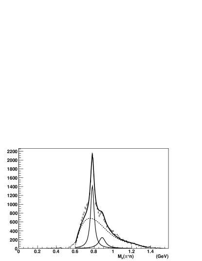
Figure 17: The missing mass off the $\pi_{2}^{+}$-$n$ combination with the $|M(\pi_{1}^{+}\pi^{-})-M_{K^{0}}|<0.01$ GeV, $|M(\pi_{2}^{+}n)-M_{\Sigma^{+}}|<0.01$ GeV, and $|M^{2}_{x}-M^{2}_{\pi^{0}}|<0.0175$ GeV² cuts. The resulting $K^{*0}$ and $\omega$ peaks are fit with Breit-Wigner line shapes, while the background is fit with a polynomial function.

The total number of $K^{*0}$ events present in the data set using the less restricted set of cuts just described can be expressed as

$$N(K^{*0})=$$

$$\frac{n(K^{*0}\to\pi^{+}\pi^{-}\pi^{0})}{R(K^{*0}\to\pi^{+}\pi^{-}\pi^{0})A^{K^{*0}}(K^{*0}\to\pi^{+}\pi^{-}\pi^{0})}=$$

$$3.639\times 10^{6}\pm 6.6\times 10^{4},$$ (13)

where $n(K^{*0}\to\pi^{+}\pi^{-}\pi^{0})=3019\pm 55$ is the estimated number of $\gamma p\to K^{*0}\Sigma^{+}\to\pi^{+}\pi^{-}\pi^{0}\pi^{+}n$ events found through the integrated fit to the $K^{*0}$ in Fig. 17. $R(K^{*0}\to\pi^{+}\pi^{-}\pi^{0})=1/3$ is the probability for the decay and $A^{K^{*0}}(K^{*0}\to\pi^{+}\pi^{-}\pi^{0})$ is the acceptance of the $K^{*0}\to\pi^{+}\pi^{-}\pi^{0}$ channel found by observing how many thrown events survive the three cuts used to obtain the $K^{*0}$ sample. The value $N(K^{*0})$ can then be used to obtain an estimate of the $K^{*0}$ contribution from any set of cuts, given an accurate acceptance for the new cuts. The number of $K^{*0}$ events that would be present in the analysis outlined in Table 1 under the $\pi^{0}$ hypothesis can be expressed as

$$N_{\pi}(K^{*0}\to\pi^{+}\pi^{-}\pi^{0})=$$

$$\frac{A_{\pi}(K^{*0}\to\pi^{+}\pi^{-}\pi^{0})n(K^{*0}\to\pi^{+}\pi^{-}\pi^{0})}{R(K^{*0}\to\pi^{+}\pi^{-}\pi^{0})A^{K^{*0}}(K^{*0}\to\pi^{+}\pi^{-}\pi^{0})},$$ (14)

where $A^{K^{*0}}(K^{*0}\to\pi^{+}\pi^{-}\pi^{0})$ is the acceptance for the $\gamma p\to K^{*0}\Sigma^{+}\to\pi^{+}\pi^{-}\pi^{0}\pi^{+}n$ channel under the $\Sigma^{+}(\pi^{0})$ hypothesis. Likewise for the $\Sigma^{+}(\gamma)$ hypothesis interchanging $A_{\pi}(K^{*0}\to\pi^{+}\pi^{-}\pi^{0})$ with $A_{\gamma}(K^{*0}\to\pi^{+}\pi^{-}\pi^{0})$ to obtain $N_{\gamma}(K^{*0}\to\pi^{+}\pi^{-}\pi^{0})$. The $K^{*0}$ radiative decay can also have a contribution under the $\Sigma^{+}(\pi^{0})$ hypothesis,

$$N_{\pi}(K^{*0}\to\pi^{+}\pi^{-}\gamma)=$$

$$R(K^{*0}\to\pi^{+}\pi^{-}\gamma)A_{\pi}(K^{*0}\to\pi^{+}\pi^{-}\pi^{0})N(K^{*0}),$$ (15)

or under the $\Sigma^{+}(\gamma)$ hypothesis,

$$N_{\gamma}(K^{*0}\to\pi^{+}\pi^{-}\gamma)=$$

$$R(K^{*0}\to\pi^{+}\pi^{-}\gamma)A_{\gamma}(K^{*0}\to\pi^{+}\pi^{-}\pi^{0})N(K^{*0}),$$ (16)

where $R(K^{*0}\to\pi^{+}\pi^{-}\gamma)=2.39\pm 0.21\times 10^{-3}$ pdg .

In the case of the $\omega$ contributions, no distinction is made between the $\gamma p\to\omega\Delta^{+}$ and $\gamma p\to\omega n\pi^{+}$ channels. The Monte Carlo used in the background estimate for the $\omega$ is the $\gamma p\to\omega\Delta^{+}$ channel only because there is a slightly larger acceptance for this channel. By using the channel of greatest acceptance an over-estimate is expected. The total number of events from $\omega\Delta^{+}\rightarrow\pi^{+}\pi^{-}\pi^{0}n\pi^{+}$ present is estimated as

$$N(\omega)=$$

$$\frac{n(\omega\to\pi^{+}\pi^{-}\pi^{0})}{R(\omega\to\pi^{+}\pi^{-}\pi^{0})A^{\omega}(\omega\to\pi^{+}\pi^{-}\pi^{0})}=$$

$$5.296\times 10^{7}\pm 4.7\times 10^{5}.$$ (17)

Here $n(\omega\to\pi^{+}\pi^{-}\pi^{0})=11120\pm 106$ is the estimate from integrating the $\omega$ fit in Fig. 17, $R(\omega\to\pi^{+}\pi^{-}\pi^{0})=89.2\pm 0.7\%$ is the branching ratio of the $\omega$ decay to $\pi^{+}\pi^{-}\pi^{0}$ pdg and $A^{\omega}(\omega\to\pi^{+}\pi^{-}\pi^{0})$ is the probability that this decay channel will be observed after the three cuts used to obtain the fit to the $\omega$ peak. An estimate of the number of counts under the $\Sigma^{+}(\pi^{0})$ hypothesis coming from the $\omega$ is obtained using Eq. 17 as

$$N_{\pi}(\omega\to\pi^{+}\pi^{-}\pi^{0})=$$

$$A_{\pi}(\omega\to\pi^{+}\pi^{-}\pi^{0})R(\omega\rightarrow\pi^{+}\pi^{-}\pi^{0})N(\omega),$$ (18)

where $A_{\pi}(\omega\to\pi^{+}\pi^{-}\pi^{0})$ is the acceptance for the $\gamma p\to\omega\Delta^{+}\to\pi^{+}\pi^{-}\pi^{0}\pi^{+}n$ channel under the $\Sigma^{+}(\pi^{0})$ hypothesis.

It is possible to express all other associated $\omega$ corrections to be obtained given the value of $N_{\omega}$, along with the acceptance terms for that particular channel. The corrections for the $\gamma$ and $\pi$ channels, respectively, are written as

$$N_{\gamma,\pi}(\omega\rightarrow\pi^{+}\pi^{-}\pi^{0}\pi^{0}) =$$

$$A_{\gamma,\pi}(\omega\rightarrow\pi^{+}\pi^{-}\pi^{0}\pi^{0})R(\omega\rightarrow\pi^{+}\pi^{-}\pi^{0}\pi^{0})N(\omega),$$

$$N_{\gamma,\pi}(\omega\rightarrow\pi^{+}\pi^{-}\gamma) =$$

$$A_{\gamma,\pi}(\omega\rightarrow\pi^{+}\pi^{-}\gamma)R(\omega\to\pi^{+}\pi^{-}\gamma)N(\omega),$$

$$N_{\gamma,\pi}(\omega\rightarrow\pi^{+}\pi^{-}\pi^{0}) =$$

$$A_{\gamma,\pi}(\omega\rightarrow\pi^{+}\pi^{-}\pi^{0})R(\omega\rightarrow\pi^{+}\pi^{-}\pi^{0})N(\omega).$$ (19)

where $R$ is used for the corresponding branching ratio or upper limit in each case, for example, $R(\omega\to\pi^{+}\pi^{-}\gamma)$ is the branching ratio for the radiative decay of the $\omega$ with a value less than $3.6\times 10^{-3}$. The value of $R(\omega\rightarrow\pi^{+}\pi^{-}\pi^{0}\pi^{0})$ is listed at less than $2\times 10^{-4}$ pdg . All results from background contributions are tabulated in Table 3. All non-listed background is considered negligible.

Table 3: The contributions for all of the background channels taken into consideration. The uncertainties are statistical only. The two columns contain the contributions estimated for each hypothesis $N_{\gamma}$, $N_{\pi}$.

Reaction	$N_{\pi}$	$N_{\gamma}$
$K^{*0}\Sigma^{+}\rightarrow K^{0}\Sigma^{+}\pi^{0}$	28.02$\pm$2.84	6.02$\pm$1.34
$K^{*0}\Sigma^{+}\rightarrow K^{0}\Sigma^{+}\gamma$	0.0157$\pm$0.0046	0.162$\pm$0.023
$\omega\Delta^{+}\rightarrow\pi^{+}\pi^{-}\pi^{0}n\pi^{+}$	$11.81\pm 2.37$	$0.0120\pm 0.0024$
$\omega\Delta^{+}\rightarrow\pi^{+}\pi^{-}\gamma n\pi^{+}$	$0.0400\pm 0.0057$	$2.1\times 10^{-5}\pm 3.0\times 10^{-6}$
$\omega\Delta^{+}\rightarrow\pi^{+}\pi^{-}\pi^{0}\pi^{0}n\pi^{+}$	$1.1\times 10^{-4}\pm 2.0\times 10^{-5}$	0.0

V.1 Final yields

To calculate the ratio of the EM decay to the strong decay, Eq. 9 is employed. All terms that take into account any channel other than the $\pi^{0}$ and radiative signals are for the time being ignored. The acceptance values are taken from Table 2. The raw values obtained out of the final kinematic fit are $n_{\gamma}=148$ and $n_{\pi}=682$, as seen in Fig. 16, with statistical uncertainties taken as the square root of $n$ in each case. After accounting for the backgrounds listed in Table 3, the corrected counts are $\Delta n_{\gamma}=135.81\pm 11.99$ and $\Delta n_{\pi}=642.11\pm 26.38$.

The ratio of the $K^{0}\Sigma^{*+}\rightarrow K^{0}\Sigma^{+}\gamma$ channel to the $K^{0}\Sigma^{*+}\rightarrow K^{0}\Sigma^{+}\pi^{0}$ channel is then,

$$R^{\Sigma^{*+}\to\Sigma^{+}\gamma}_{\Sigma^{*+}\to\Sigma^{+}\pi^{0}} = \frac{\Delta n_{\gamma}A_{\pi}(\Sigma\pi)-\Delta n_{\pi}A_{\gamma}(\Sigma\pi)}{\Delta n_{\pi}A_{\gamma}(\Sigma\gamma)-\Delta n_{\gamma}A_{\pi}(\Sigma\gamma)}$$ (20)

$$= 11.95\pm 2.21\%.$$

The raw counts for the radiative and $\pi^{0}$ extraction were obtained using $P^{a}_{\gamma}=P^{a}_{\pi}<0.01\%$ with the final confidence level cut $P^{b}_{\gamma}=P^{b}_{\pi}>10\%$ as mentioned in the cuts from Table 1.

Only the statistical uncertainty is quoted. To determine how reliable the ratio is a set of systematic studies is required along with a study of the variation in the ratio based on the choice of confidence level cuts. This variation and all other systematic studies are considered in the next section.

VI Systematic Studies

The value of each of the nominal cuts was varied to study the effect on the final background corrected ratio. For each variation the new acceptance terms in Equation 9 were recalculated with the corresponding Monte Carlo. Each major systematic uncertainty contribution is numbered as it is discussed and listed in Table 8, which contains a summary of all systematic uncertainties.

Several $\Delta\beta$ cut variations were checked starting with $|\Delta\beta|<0.02$ for all charged particles, leading to a ratio of 11.98$\pm$2.22$\%$. There was also a check at $|\Delta\beta|<0.1$ that gave a ratio of 11.74$\pm$2.17%. The $|\Delta\beta|$ cut selected uses a $\pm 1$ ns timing cut, while keeping $|\Delta\beta|<0.035$ for all pions. This variation is presented in Table 8 as number (1).

To estimate the systematic effects from the Monte Carlo, such as the uncertainty in correctly simulating the data, a comparison was made with the cross section of $\gamma p\to K^{0}\Sigma^{*+}$ from Monte Carlo and data. The ratio was obtained using the acceptance corections based on a Monte Carlo with a zero $t$-slope in the generator to get $R=11.70\pm$2.21$\%$. This value deviated from the ratio obtained by $\sim 2\%$. The uncertainty from Monte Carlo was then estimated to be $\sim 2\%$ in either direction. This finding leads to a high value in the ratio of $R=12.19\pm$2.21$\%$ and a lower value in the ratio of $R=11.71\pm$2.21$\%$, which is listed as number (2) in Table 8.

The missing energy cut removes a large amount of background that slips in under the $\Sigma^{*+}$. The final cut of $E_{x}<0.24$ GeV was chosen based on the maximization of signal counts (decreased statistical uncertainty). The systematic contribution for the $E_{x}$ cut was studied by varying the cut in a reasonable range about the nominal value. This ratio was reasonably stable up until $E_{x}<0.28$ GeV, at which point the $\pi^{0}$ and $\gamma$ signals become overwhelmed with background. Cuts in $E_{x}$ too low in energy tend to distort the ratio. Based on this study a high ($11.95\pm$2.21$\%$) and low ($11.71\pm$2.20$\%$) value were assigned to the associated systematic uncertainties. These contributions are listed in Table 8 as number (3).

The background counts that contribute to the ratio assume a branching ratio for $\omega\to\pi^{+}\pi^{-}\gamma$ to be at the top of the upper limit at $3.6\times 10^{-3}$, as well as for $\omega\to\pi^{+}\pi^{-}\pi^{0}\pi^{0}$ at $2\times 10^{-4}$ pdg . The variation in uncertainty of the branching ratio of either of these channels is not of large enough order to make a notable effect on the ratio. The total contribution from background in the $\pi^{0}$ hypothesis was $39.89\pm 3.70$ and for the $\gamma$ hypothesis was $6.19\pm 1.34$. To check for the largest deviations under these uncertainties, a contribution of 43.59 counts from the $\pi^{0}$ hypothesis was used with 4.85 counts for the $\gamma$ hypothesis, leading to a ratio of $12.37\pm 2.24\%$. The opposite extreme was also used to obtain 36.19 counts from the $\pi^{0}$ hypothesis and 7.5 counts for the $\gamma$ hypothesis, leading to a ratio $11.54\pm 2.19\%$. This finding is listed in Table 8 as number (4).

The kinematic fits used to control the leakage of the $K^{*0}$ and $\omega$ have an associated confidence level cut that was also tested. The cut in each case was selected based on the reduction of the specific background channel, while maximizing the signal counts from the $\gamma$ and $\pi^{0}$. A check was done over a large range of confidence level cuts for each case to test the variation in the ratio. New background contributions were found for each cut along with new acceptance terms. The ratio was then recalculated and tabulated for the $K^{*0}$ ($\omega$) removal in Table 4 (Table 5). These contributions are listed as (5) and (6), respectively, in Table 8.

$P_{\gamma}(\chi^{2})=P_{\pi}(\chi^{2})$	$R$
0.100	12.04$\pm$2.20%
0.050	11.79$\pm$2.20%
0.010	11.95$\pm$2.21%
0.005	11.92$\pm$2.22%
0.001	11.90$\pm$2.21%

Table 4: The values used in the systematic variation for the calculated ratio with respect to the confidence level cut from the fit to $\gamma p\to\pi^{+}nK^{*0}\to\pi^{+}n\pi^{+}\pi^{-}(\pi^{0})$ and $\gamma p\to\pi^{+}nK^{*0}\to\pi^{+}n\pi^{+}\pi^{-}(\gamma)$. The confidence level cuts were set equal to each other such that $P_{\gamma}(\chi^{2})=P_{\pi}(\chi^{2})$.

$P_{\gamma}(\chi^{2})=P_{\pi}(\chi^{2})$	$R$
0.100	11.99$\pm$2.20%
0.050	12.01$\pm$2.21%
0.010	11.95$\pm$2.21%
0.005	11.80$\pm$2.22%
0.001	11.77$\pm$2.21%

Table 5: The values used in the systematic variation for the calculated ratio with respect to the confidence level cut from the fit to $\gamma p\to\pi^{+}n\omega\to\pi^{+}n\pi^{+}\pi^{-}(\pi^{0})$ and $\gamma p\to\pi^{+}n\omega\to\pi^{+}n\pi^{+}\pi^{-}(\gamma)$. The confidence level cuts were set equal to each other such that $P_{\gamma}(\chi^{2})=P_{\pi}(\chi^{2})$.

The optimum set of confidence level cuts used to extract the final yields has a range of validity in which a study of the ratio variation is appropriate. The range of validity is found by using the fractional deviation in the ratio $\delta R$, and requiring it to be less than or equal to the fractional uncertainty due to statistics. $\delta R$ is defined as the difference in the generated ratio and recovered ratio in the Monte Carlo study. The set of optimum cuts occurs at different values for a given mixture of Monte Carlo $\Sigma^{+}\pi^{0}$ and $\Sigma^{+}\gamma$ events. Using the $g11a$ data, the Monte Carlo was tuned to have approximately the same ratio and the same statistics as the real data, and the optimum cuts were thereby determined quantitatively. This set of cuts used in the systematic studies, along with the values of $\delta R$, are given in Table 6 for isolation of the radiative decay and Table 7 for the $\pi^{0}$ isolation. Note that the value of $\delta R$ is not the systematic uncertainty in $R^{\Sigma^{+}\gamma}_{\Sigma^{+}\pi}$. Rather, the systematic uncertainty comes from the data ratio values in the right-most column in each table. The systematic uncertainty is based on the variation in the extracted ratio of Eq. (LABEL:R) for a set of cuts determined to give the minimal deviation in the Monte Carlo recovered ratio for the valid range of statistics.

$P^{a}_{\pi}(\%)$	$P^{b}_{\gamma}(\%)$	$\delta$$R$	$R$
0.050	17	0.140	11.68$\pm$2.22%
0.005	15	0.090	11.88$\pm$2.29%
0.010	10	0.089	11.95$\pm$2.21%
0.075	20	0.092	11.41$\pm$2.27%

Table 6: Optimization points for each $P^{a}_{\pi}$ and $P^{b}_{\gamma}$ for the $\Sigma^{+}\gamma$ channel.

$P^{a}_{\gamma}(\%)$	$P^{b}_{\pi}(\%)$	$\delta$$R$	$R$
0.050	17	0.187	11.35$\pm$2.23%
0.005	15	0.109	12.13$\pm$2.31%
0.010	10	0.099	11.95$\pm$2.21%
0.075	20	0.195	11.19$\pm$2.30%

Table 7: Optimization points for each $P^{a}_{\gamma}$ and $P^{b}_{\pi}$ for the $\Sigma^{+}\pi^{0}$ channel.

The systematic dependence on the choice of the $P(\chi^{2})$ cuts in both the radiative and $\pi^{0}$ hypotheses comes from Table 6 and Table 7. The ratio was recalculated from the resulting raw counts in each case with the new acceptance terms for the set of cuts obtained from the optimal range. The set of cuts was tested for both the radiative and $\pi^{0}$ hypotheses separately. In each variation under the $\pi^{0}$ ($\gamma$) hypothesis, the opposing cut for the $\gamma$ ($\pi^{0}$) hypothesis was not changed. The highest and lowest value from each study were used as the contributions to the systematic uncertainty listed as (7) and (8) in Table 8.

The cut on the $\pi_{1}^{+}$-$\pi^{-}$ invariant mass was used to minimize the events that are not associated with a $K^{0}$. A range of cuts on $|M(\pi_{1}^{+}\pi^{-})-M_{K^{0}}|$ was used to study this effect. Only the stable region was used in the final determination of the range of variation for this cut with a high value of 11.95$\pm$2.21% and a low value of 11.72$\pm$2.21%. These are listed in line (9) of Table 8.

The cut on the $\pi_{2}^{+}$-$n$ invariant mass regulates the candidates going into the final set of kinematic fits so there is some sensitivity to any events that do not come from the $\Sigma^{+}$. A range of cuts on $|M(\pi_{2}^{+}n)-M_{\Sigma^{+}}|$ was used to study this effect. Only the stable region was used in the final determination of the range of variation for this cut with a high value of 11.95$\pm$2.21% and a low value of 11.34$\pm$2.85%. These are listed in line (10) of Table 8.

Table 8 shows a summary of the systematic studies and the highest and lowest value of the ratio based on the variations mentioned for each type of uncertainty.

Table 8: Sources of systematic variation in the ratio (in %) showing the contributions to the systematic uncertainties from changes to the event selection values, along with the low and high value used.

Source	Low Value	Low Contribution	High Value	High Contribution
(1) $\Delta\beta$	11.74$\pm$2.17	-0.21	11.98$\pm$2.22	+0.03
(2) MC-match	11.71$\pm$2.21	-0.24	12.19$\pm$2.21	+0.24
(3) $E_{x}$	11.71$\pm$2.20	-0.24	$11.95\pm$2.21	+0.00
(4) BG uncertainty	11.54$\pm$2.19	-0.41	12.37$\pm$2.24	+0.42
(5) $K^{*0}$-CL	11.79$\pm$2.20	-0.16	12.04$\pm$2.20	+0.09
(6) $\omega$-CL	11.77$\pm$2.21	-0.18	12.01$\pm$2.21	+0.06
(7) $\gamma$-CL	11.41$\pm$2.27	-0.54	11.95$\pm$2.21	+0.00
(8) $\pi^{0}$-CL	11.35$\pm$2.23	-0.60	12.13$\pm$2.31	+0.18
(9) $K^{0}$ cut	11.72$\pm$2.21	-0.23	11.95$\pm$2.21	+0.00
(10) $\Sigma^{+}$ cut	11.34$\pm$2.85	-0.61	11.95$\pm$2.21	+0.00
Total Uncertainty		-1.21		+0.53

To calculate the final systematic uncertainty, the difference in the ratio $R=11.95\%$ and the high value of the ratio for each case in Table 8 was added in quadrature to obtain a value for the uncertainty of 0.53% greater than the ratio. The lower systematic uncertainty bound was based on the difference between the ratio $R=11.95\%$ and the low value of the ratio for each case, resulting in a value of 1.21% less than the ratio. The final ratio reported is $11.95\pm 2.21(stat)_{-1.21}^{+0.53}(sys)\%$.

VII Overall Results

The final result for the ratio of the $\Sigma^{*+}\to\Sigma^{+}\gamma$ to $\Sigma^{*+}\to\Sigma^{+}\pi^{0}$ with systematic uncertainties is

$$R^{\Sigma^{*+}\to\Sigma^{+}\gamma}_{\Sigma^{*+}\to\Sigma^{+}\pi^{0}}=\frac{n_{\gamma}A_{\pi}(\Sigma\pi)-n_{\pi}A_{\gamma}(\Sigma\pi)}{n_{\pi}A_{\gamma}(\Sigma\gamma)-n_{\gamma}A_{\pi}(\Sigma\gamma)}=$$

$$11.95\pm 2.21(stat)_{-1.21}^{+0.53}(sys)\%.$$ (21)

To calculate the EM decay partial width from the measured branching ratio, the full width of the $\Sigma^{*+}$ decay is used, $\Gamma_{Full}=35.8\pm 0.8$ MeV pdg , with the branching ratio $R(\Sigma^{*+}\to\Sigma^{+}\pi^{0})=5.85\pm 0.75\%$. The partial width calculation including systematic uncertainties leads to,

$$\Gamma_{\Sigma^{*+}\to\Sigma^{+}\gamma}=R^{\Sigma^{*+}\to\Sigma^{+}\gamma}_{\Sigma^{*+}\to\Sigma^{+}\pi^{0}}R(\Sigma^{*}\to\Sigma^{+}\pi^{0})\Gamma_{Full}=$$

$$250\pm 56.9(stat)_{-41.2}^{+34.3}(sys)\text{ keV}.$$ (22)

To obtain the corresponding U-spin prediction, we first look at the prediction for the $\Delta^{+}\to p\gamma$ partial width to the $\Sigma^{*+}\to\Sigma^{+}\gamma$ partial width.

$$\left\langle\Delta^{+}|p\gamma\right\rangle = \left\langle\frac{1}{2}-\frac{1}{2}|\frac{1}{2}-\frac{1}{2}~{}0~{}~{}0\right\rangle=1$$

$$\left\langle\Sigma^{*+}|\Sigma^{+}\gamma\right\rangle = \left\langle\frac{1}{2}+\frac{1}{2}|\frac{1}{2}-\frac{1}{2}~{}0~{}~{}0\right\rangle=1,$$

leading to a ratio of,

$$\frac{\Gamma(\Delta^{+}\to p\gamma)}{\Gamma(\Sigma^{*+}\to\Sigma^{+}\gamma)}=\left(\frac{M_{p}}{M_{\Delta}}\right)\left(\frac{M_{\Sigma^{+}}}{M_{\Sigma^{*+}}}\right)^{-1}\left(\frac{q_{p}}{q_{\Sigma^{+}}}\right)^{3}=2.638.$$

The value for the center of mass momentum for the proton is $q_{p}=0.259$ GeV and for the $\Sigma^{+}$ is $q_{\Sigma}^{+}=0.180$ GeV, pdg .

This implies that the U-spin prediction for the partial width of the electromagnetic decay using the $660\pm 60$ MeV width of the $\Delta^{+}\to p\gamma$ decay pdg is,

$$\frac{\Gamma(\Delta^{+}\to p\gamma)}{2.638}=250\pm 23\text{ keV}.$$ (23)

A similar calculation can be done for to obtain a U-spin prediction for the $\Gamma_{\Sigma^{*0}\to\Lambda\gamma}$ partial decay width. Table 9 shows the previous model predictions along with the U-spin prediction and the final results from this analysis in each case. The statistical and systematic uncertainties are combined in the present partial widths.

Table 9: Comparison of theoretical model predictions for the radiative decay widths with the experimental result for $\Sigma^{*0}$ from Ref. kellpaper and the present result result for $\Sigma^{*+}$.

Model	$\Sigma(1385)^{0}\to\Lambda\gamma$	$\Sigma^{+}(1385)\to\Sigma^{+}\gamma$
NRQM DHK ; Koniuk ; kaxiras	273	104
RCQM warns	267
$\chi$CQM wagner	265	105
MIT Bag kaxiras	152	117
Soliton Schat	243	91
Skyrme Abada ; Haberichter	157-209	47
Algebraic model Bijker	221.3	140.7
U-spin	423$\pm$38	250$\pm$23
Results	445$\pm$102	250$\pm$70

The partial width in both cases is larger than any prediction listed except for the U-spin prediction. The U-spin predictions for the $\Sigma^{*0}\to\Lambda\gamma$ and $\Sigma^{*+}\to\Sigma^{+}\gamma$ partial widths are well validated by the experimental result. For these cases U-spin symmetry is confirmed within the experimental uncertainties. It is important to note that the U-spin prediction for the $\Sigma^{*+}$ EM decay partial width ignores the effects of the interference of the isovector and isoscalar components of the photon. If the isoscalar component interfered destructively, the resulting prediction could indeed be much smaller.

The results in Ref. lee2 reveal that the meson cloud effect can contribute significantly ($\sim 40\%$) to the overall electromagnetic decay width of the $\Delta\to N\gamma$. This puts the prediction from the model at about $80\%$ of the experimental measurement. As stated previously it has not yet been determined from a theoretical standpoint if the meson cloud effects contribute and if so to what degree for the radiative decay of the $\Sigma^{*0}$ and $\Sigma^{*+}$. This may be the reason for such a difference in the predictions seen from experiment compared to the models listed in Table 9. Because the U-spin prediction for the $\Sigma^{*}$ EM decay width uses empirical information from the $\Delta$ EM decay, contributions from phenomena like the meson cloud effect should be inherent. The correspondence between the U-spin prediction and the experimental result strongly suggests that the other models lack that corresponding effect.

Perhaps this work can prompt more encompassing calculations that are necessary to probe the structure of the baryon resonances and motivate consideration of the meson cloud contributions for electromagnetic decay predictions.

VIII Acknowledgment

The authors thank the staff of the Thomas Jefferson National Accelerator Facility who made this experiment possible. This work was supported in part by the Chilean Comisión Nacional de Investigación Científica y Tecnológica (CONICYT), the Italian Istituto Nazionale di Fisica Nucleare, the French Centre National de la Recherche Scientifique, the French Commissariat à l’Energie Atomique, the U.S. Department of Energy, the National Science Foundation, the UK Science and Technology Facilities Council (STFC), the Scottish Universities Physics Alliance (SUPA), the United Kingdom’s Science and Technology Facilities Council, and the National Research Foundation of Korea.

The Southeastern Universities Research Association (SURA) operates the Thomas Jefferson National Accelerator Facility for the United States Department of Energy under contract DE-AC05-84ER40150.

References

- (1) N. Isgur and G. Karl, Phys. Lett. B 72, 109 (1977).
- (2) N. Isgur and G. Karl, Phys. Rev. D 18, 4187 (1978).
- (3) J. W. Darewych, M. Horbatsch, and R. Koniuk, Phys. Rev. D 28, 1125 (1983).
- (4) R. Koniuk and N. Isgur, Phys. Rev. D 21, 1868 (1980); Erratum: ibid. 23, 818 (1981).
- (5) M. Warns, W. Pfeil, and H. Rollnik, Phys. Lett. B 258, 431 (1991).
- (6) G. Wagner, A. J. Buchmann, and A. Faessler, Phys. Rev. C 58, 1745 (1998).
- (7) E. Kaxiras, E.J. Moniz, and M. Soyeur, Phys. Rev. D 32, 695 (1985).
- (8) C. L. Schat, C. Gobbi, and N. B. Scoccola, Phys. Lett. B 356, 1 (1995).
- (9) A. Abada, H. Weigel, and H. Reinhardt, Phys. Lett. B 366, 26 (1996).
- (10) T. Haberichter, H. Reinhardt, N. N. Scoccola, and H. Weigel, Nucl. Phys. A 615, 291 (1997).
- (11) R. Bijker, F. Iachello, and A. Leviatan, Annals Phys. 284, 89 (2000).
- (12) D. Keller et al. (CLAS Collaboration), Phys. Rev. D 83, 072004 (2011).
- (13) S. Taylor et al. (CLAS Collaboration), Phys. Rev. C 71, 054609 (2005).
- (14) B. Juliá-Díaz, T.-S.H. Lee, T. Sato, and L.C. Smith, Phys. Rev. C 75, 015205 (2007).
- (15) N. Isgur and G. Karl, Phys. Rev. D 20, 1191 (1979).
- (16) H. Lipkin, Phys. Rev. D 7, 846 (1973).
- (17) H. Lipkin and M. Moinester, Phys. Lett. B 287, 179 (1992).
- (18) R. Dashen and A.V. Manohar, Phys. Lett. B 315, 425 (1993).
- (19) D. Leinweber, T. Draper, and R. Woloshyn, Phys. Rev. D 48, 2230 (1993).
- (20) V. V. Molchanov et al. (SELEX Collaboration), Phys. Lett. B 590, 161 (2004).
- (21) B. A. Mecking et al., Nucl. Instrum. Meth. A 503, 513 (2003).
- (22) D. I. Sober et al., Nucl. Instrum. Meth. A 440, 263 (2000).
- (23) M. E. McCracken et al. (CLAS Collaboration), Phys. Rev. C 81 025201 (2010).
- (24) Review of Particle Properties, J. Phys. G 37, 075021 (2010).
- (25) M. Amarian et al., Nucl. Inst. Meth. A 440, 263 (2000).
- (26) D. Keller “Techniques in Kinematic Fitting”, CLAS-NOTE 2010-015.
- (27) D. Keller “EC Neutron Covariance”, CLAS-NOTE 2011-001.
- (28) J. W. C. McNabb. “Photoproduction of and hyperons off Protons in the Nucleon Resonance Region using CLAS at Jefferson Lab”. Ph.D. Thesis, Carnegie Mellon University (2004).
- (29) CERN-CN Division, GEANT 3.2.1, CERN Program Library W5013 (1993).
- (30) T. Sato and T.-S. H. Lee, Phys. Rev. C 54, 2660 (1996).