Superradiance Transition in Photosynthetic Light-Harvesting Complexes

Abstract

We investigate the role of long-lasting quantum coherence in the efficiency of energy transport at room temperature in Fenna-Matthews-Olson photosynthetic complexes. The excitation energy transfer due to the coupling of the light harvesting complex to the reaction center (“sink”) is analyzed using an effective non-Hermitian Hamiltonian. We show that, as the coupling to the reaction center is varied, maximal efficiency in energy transport is achieved in the vicinity of the superradiance transition, characterized by a segregation of the imaginary parts of the eigenvalues of the effective non-Hermitian Hamiltonian. Our results demonstrate that the presence of the sink (which provides a quasi–continuum in the energy spectrum) is the dominant effect in the energy transfer which takes place even in absence of a thermal bath. This approach allows one to study the effects of finite temperature and the effects of any coupling scheme to the reaction center. Moreover, taking into account a realistic electric dipole interaction, we show that the optimal distance from the reaction center to the Fenna-Matthews-Olson system occurs at the superradiance transition, and we show that this is consistent with available experimental data.

I Introduction

The annual amount of energy humans currently use is delivered to Earth by the Sun in a few hours! Since solar energy is very dilute, it is essential to transport the captured energy efficiently. Most natural photosynthetic systems consist of antenna complexes, which capture photons from the Sun and transport energy to a reaction center (RC). There, it is transformed into chemical energy via charge separation. Antenna complexes are able to transfer excitations to RCs with an efficiency exceeding $95\%$. For a long time, it was thought that energy transfer in photosynthetic light-harvesting complexes occurs through classical processes, similar to random walks of the exciton to the RC. However, surprising evidence of coherent quantum energy transfer has been found recently photo ; photoT . These findings raise two basic questions. How can coherence be maintained in complex biological systems at room temperature? Why is quantum coherence relevant to the efficiency of energy transfer?
The first question has been addressed in photo2 ; photo3 . We consider here the second one. It is known that quantum coherence can speed up energy transport through a quantum walk, which can be faster than a classical walk qwalk . Although the relevance of a mechanism similar to Dicke superradiance dicke54 has been also pointed out in srlloyd ; sr2 , we focus here on a different feature of the “superradiance transition” (ST) SZNPA89 ; Zannals . We show that ST is a dominant mechanism in an antenna complex described by discrete energy levels coupled to the RC, modeled here by a sink having a continuum energy spectrum similar to what has been done in photo2 ; qwalk ; cechi . On the other hand, the effects of the thermal bath lead only to small corrections to the energy transport in the vicinity of maximal efficiency. The antenna-sink coupling causes the appearance of a resonance width (inverse of life-time) and an energy (Lamb) shift. For weak coupling strength, the resonance widths are roughly the same. However, if the coupling strength reaches a critical value, at which the resonance widths start to overlap, then a segregation of widths builds up. In this regime, almost the entire (summed up) decay width is allocated to just a few short-lived “superradiant states”, while all other states are long-lived (and effectively decoupled from the environment). We call this segregation the “Superradiance Transition”. This effect has been studied using random matrix theory verbaarschot85 ; puebla , in nuclear physics Volya , for microwave billiards rotter2 and in paradigmatic models of coherent quantum transport kaplan ; rottertb . It was shown in kaplan that in a realistic model for quantum transport, maximum transmission is achieved at ST.
In this paper, we focus on transport properties of the Fenna-Matthews-Olson (FMO) complex, found in green sulphur bacteria. This complex, one of the most studied in the literature photo2 ; photo3 ; qwalk ; renaud , acts as a conductor for energy transport between the antenna system and the RC. The FMO complex is a dissipative open quantum system which interacts with the thermal bath provided by the protein environment. Here we take an effective non-Hermitian Hamiltonian approach MW ; SZNPA89 ; Zannals and study the ST as a function of the coupling to the RC and the thermal bath, due to phonons. The phonon bath induces dephasing and dissipation, and we take both effects into account using two different models for the phonon bath. Since ST is due to quantum coherence, we address here two main issues: i) whether its effects can survive in presence of dephasing induced by the phonon bath at room temperature, and ii) how ST depends on the strength of the coupling between the FMO and the RC. It has been shown recently that maximal transport efficiency for the FMO complex is achieved near a critical coupling to the RC mohseni . However, so far, the dependence of this critical coupling on the parameters of the FMO and the RC has not been determined. We compute this critical coupling analytically and show that it corresponds to the ST. We demonstrate that the quantum coherent effect of ST, even taking into account dephasing and relaxation, determines the maximal transport efficiency at room temperature. Indeed, the ST is due to coherent constructive interference between the various paths to the RC, thus enhancing the rate of energy transfer. Finally, with the aid of the non-Hermitian Hamiltonian approach, we consider a realistic coupling between the FMO complex and the RC, showing that the ST determines the optimal distance from the RC to the FMO system.

II The Model for Superradiance transition

The FMO complex is a trimer, composed of identical subunits, each of which contains seven bacteriochlorophylls (BChl) 8Bchl . Each subunit acts independently and can be modelled using a tight-binding Hamiltonian,

$$H_{0}=\sum_{i=1}^{7}E_{i}|i\rangle\langle i|+\sum_{i,j}(J_{i,j}|i\rangle\langle j|+h.c.).$$ (1)

Here, $|i\rangle$ is the state in which the $i$-th site is excited and the others are in the ground state. Since the solar energy is very dilute, we limit the description to a single excitation in the complex, as is commonly done in the literature. The numerical values of $E_{i}$ and $J_{i,j}$ have been taken from Ref. photo2 . Below we take the matrix elements of $H_{0}$ expressed in $cm^{-1}$:

$$\left(\matrix{200&-87.7&5.5&-5.9&6.7&-13.7&-9.9\cr-87.7&320&30.8&8.2&0.7&11.8&4.3\cr 5.5&30.8&0&-53.5&-2.2&-9.6&6\cr-5.9&8.2&-53.5&110&-70.7&-17&-63.3\cr 6.7&0.7&-2.2&-70.7&270&81.1&-1.3\cr-13.7&11.8&-9.6&-17&81.1&420&39.7\cr-9.9&4.3&6&-63.3&-1.3&39.7&230\cr}\right)$$

The incident photon creates an electron-hole pair, called an exciton, which decays due to two processes: coupling to the electromagnetic field, i.e. emission of a photon (recombination) with an associated decay time, $T_{1}$, and coupling to the RC with a decay time, $T_{1r}$.
As is common in quantum optics milonni , we describe this dissipative system with at most one excitation by states

$$|\psi\rangle=\sum_{i=1}^{7}a_{i}|0\rangle\otimes|i\rangle+\sum_{c}\int dE\ b_{c}(E)|c,E\rangle\otimes|gs\rangle,$$ (2)

where $|0\rangle$ is the vacuum state of the environment and $|c,E\rangle\otimes|gs\rangle$ is the state with one excitation in the environment and none on the sites. Here, $c$, is the quantum number labelling channels (at energies $E$) in the environments. The reduced density matrix is obtained by tracing over the states $|0\rangle$ and $|c,E\rangle$,

$$\rho = \sum_{i,j}a_{i}a_{j}^{*}|i\rangle\langle j|+(1-\sum_{i}|a_{i}|^{2})|gs\rangle\langle gs|,$$ (3)

which is an $8\times 8$ matrix. However, $\langle gs|\rho|i\rangle=0$ since with the choice (2), we neglect the transitions $|i\rangle\to|gs\rangle$. Moreover, $\langle gs|\rho|gs\rangle$ is simply the loss of probability of excitation of the seven sites. Therefore, we restrict our considerations to the $7\times 7$ matrix $\langle i|\rho|j\rangle$, $1\leq i,j\leq 7$, which however does not have constant trace.
In order to compute the evolution of the reduced density matrix, we introduce an effective non-Hermitian Hamiltonian SZNPA89 ; kaplan ; messiah which in general can be written as, $H_{\mathrm{eff}}(E)=H_{0}+\Delta(E)-iW(E)$, where $H_{0}$ is the Hermitian Hamiltonian of the system decoupled from the environments and $\Delta(E)$ and $W(E)$ are the induced energy shift and the dissipation, respectively. Neglecting the energy dependence and the energy shift we have

$$H_{\mathrm{eff}}=H_{0}-iW\hskip 14.22636pt{\rm with}\hskip 14.22636ptW_{ij}=\sum_{c}A_{i}^{c}(A_{j}^{c})^{*}.$$ (4)

The real symmetric matrix, $W$, is given in terms of the bound state-continuum transition amplitudes, $A_{i}^{c}$, from the discrete state $i$ to the continuum channel $c$.
The Schrödinger equation and Eq. (2), result in the following equation for the coefficients, $a_{j}$:

$$i\hbar\dot{a}_{j}=\sum_{k=1}^{7}\left({H_{0}}_{jk}a_{k}-iW_{jk}a_{k}\right),$$ (5)

and from this the master equation easily follows,

$$i\hbar\dot{\rho}_{jk}=[H_{0}\,,\rho]_{jk}-i\sum_{l=1}^{7}\left(W_{jl}\rho_{lk}+\rho_{jl}W_{lk}\right).$$ (6)

Under the standard assumption lloyd ; deph that each site is coupled to an independent (local) environment, with associated coupling time $T_{1}$, we have $A_{i}^{i}=\sqrt{\hbar/2T_{1}}$, $i=1,..,7$. The site $i=3$ is the only one which is, in addition, coupled to the RC, giving rise to a decay time $T_{1r}$. Then $A_{3}^{8}=\sqrt{\hbar/2T_{1r}}$ (in this scheme there are 7+1 channels); for other channels we have $A_{i}^{c}=0$. In Eq. (6) we take into account: (i) the interaction between the FMO and the RC through the time $T_{1r}$ and (ii) the characteristic time of exciton recombination, $T_{1}$. The effects of the thermal bath will be considered in Sec.(IV).

One can verify that equation (6) can also be obtained by restriction to the $7\times 7$ density matrix, from a Lindblad dynamics for the full $8\times 8$ density matrix (3).
In the following, we fix $T_{1}=1\ ns$, which is the exciton recombination time reported in the literature lloyd ; deph , and we focus on the effect of varying $T_{1r}$.

III Superradiance transition

ST can be analyzed by studying the complex eigenvalues, ${\cal E}_{r}=E_{r}-i\Gamma_{r}/2$ of $H_{\rm eff}$, defined in (4). As the coupling between the excitonic states and the RC increases, one observes a rearrangement of the widths, $\Gamma_{r}$ (the “superradiance” transition kaplan ). We show this effect in Fig. 1 (left panel), where the largest width (red dashed curve) and the average of the $7-1=6$ smallest widths (black full curve) are plotted as functions of $T_{1r}$. For weak coupling to RC (large $T_{1r}$) the widths of all states increase as $T_{1r}$ decreases. On the other hand, below a critical value $T_{1r}^{cr}$, corresponding to ST, (vertical line), the average of the $6$ smallest widths decreases while the largest width, corresponding to the superradiant state, increases. To examine localization of the excitation we use the Participation Ratio (PR)felix of a state $|\psi\rangle$, defined as:

$$PR=(\sum_{i}|\langle i|\psi\rangle|^{4})^{-1}.$$

Its value varies from $1$ for fully localized to $7$ for fully delocalized states. The right panel of Fig. 1 shows the PR for the state associated with the largest width (the one decaying most quickly). In the superradiant regime, $T_{1r}<T_{1r}^{cr}$, this state is fully localized on site $3$, the only site connected to the RC. For weak coupling to the RC, $T_{1r}>T_{1r}^{cr}$, the PR is approximately $1.6$. This small value, as compared to the maximal possible value of $7$, is explained by (Anderson) localization Anderson of the eigenstates on sites. The Anderson localization effect in the FMO system is due to the fact that the excitation energies of the sites and the couplings among them are all different. Thus, the FMO complex can be thought of as a disordered system.

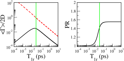
Figure 1: (Color online) Left panel: average decay width, normalized to the mean level spacing, $D$ as a function of the coupling time to the RC, $T_{1r}$. The black curve represents the average decay width of the $6$ states with smallest width, while the dashed red curve shows the largest decay width. Right panel: PR of the eigenstate of $H_{{\mathrm{eff}}}$ with the largest width as a function of $T_{1r}$. In both panels the vertical (green) line indicates the critical value of $T_{1r}$ at which ST occurs.

The critical value, $T_{1r}^{cr}$, at which ST occurs, can be estimated analytically. If all states have roughly the same width, at least for small coupling, then the superradiance condition coincides with that of overlapping resonances. Such a reasoning can be applied to the FMO system, too. Here, eigenstates are mostly localized on the sites, and only site $3$ is coupled to the RC. The widths are thus not uniform and most of the total width belongs to the eigenstate localized at site $3$. Imposing that the half width, $\Gamma_{3}/2$, is approximately equal to the mean level spacing $D$, $\Gamma_{3}/2\approx D$, and using $\Gamma_{3}\approx\hbar/T_{1r}$, we obtain the critical value at which ST occurs,

$$T_{1r}^{cr}\approx\frac{\hbar}{2D}.$$ (7)

In the FMO system, the energy level spacing is $D/hc\approx 83.5$ $cm^{-1}$, which gives $T_{1r}^{cr}\approx 0.03\ ps$, a value in very good agreement with the numerical results of Fig. 1 (vertical line).

Such a value, $T_{1r}=0.03\ ps$, corresponds to a transfer rate, $\kappa$, from site $3$ to the RC of $\kappa=\frac{1}{2T_{1r}}=16.6\ ps^{-1}$. This value is larger than the values usually mentioned in literature, which range from $0.25\ ps^{-1}$ to $4\ ps^{-1}$ deph , even if $1\ ps^{-1}$ is the most common value qwalk . This discrepancy can be due to the simplicity of our model, even if it is important to notice that, to the best of our knowledge, the real value of the coupling time, $T_{1r}$, is not exactly known. In any case, for this reason, in Section VIb, we consider a more realistic coupling scheme between the FMO system and the RC.

IV Efficiency of energy transport in presence of a thermal bath

Interaction with the phonon environment is complicated, and it involves both dephasing and dissipation photo2 . Since superradiance is due to quantum coherence, in Sec (IV.1) we first focus on dephasing and the consistent indirect relaxation, induced by the presence of classical noise. On the other hand, in Sec. (IV.2), we consider both dephasing and dissipation induced by a finite temperature bath. Needless to say, while the latter bath induces at equilibrium a Gibbs energy level distribution, the former gives rise to an equal population of all energy levels.

IV.1 Efficiency of energy transport in presence of noise

As a first step, one can study the effects of the phonon bath modelling the thermal bath by a classical noise. In this case, the dephasing effects are adequately described using an interaction as in Ref. lloyd :

$$H_{{}_{SB}}=\sum q_{i}(t)|i\rangle\langle i|,$$ (8)

with

$$\langle q_{i}(t)q_{j}(t)\rangle=\hbar^{2}\gamma_{d}\delta_{i,j}\delta(t),$$ (9)

where $\gamma_{d}$ plays the role of the dephasing rate. This approach corresponds to an effective infinite temperature that leads to equal populations of energy levels at sufficiently large times. We take into account the interaction (8) by adding a dephasing Lindblad operator to the master equation (6), as was done in Ref. [19]. The interaction with noise leads to the Haken-Strobl master equation for the density matrix of the following form:

$$\frac{d\rho_{i,j}}{dt}=-\frac{i}{\hbar}\left(H_{\mathrm{eff}}\rho-\rho H_{\mathrm{eff}}^{+}\right)_{i,j}-\gamma_{d}(1-\delta_{i,j})\rho_{i,j}.$$ (10)

The first term in the r.h.s. of Eq. (10) takes into account the coherent evolution and the dissipation by recombination and trapping into the reaction center, (it is simply Eq. (6) rewritten in terms of $H_{\mathrm{eff}}$, defined in Eq. (4)). The last term, which corresponds to the decay of the off-diagonal matrix elements, takes into account dephasing and indirect relaxation. For the FMO system, the amplitude of noise, $\hbar\gamma_{d}$, is related to the temperature, $T$, by the relation, found in experiments photoT ,

$$\hbar\gamma_{d}(T)\simeq 0.52\ \hbar c\ (T/K)(cm)^{-1},$$ (11)

where $T$ is the temperature expressed in kelvin degrees, $K$.

Transport efficiency has been measured as in Ref. deph by the probability that the excitation is in the RC at the time $t_{max}$,

$$\eta(t_{max})=\frac{1}{T_{1r}}\int_{0}^{t_{max}}\ dt\ \rho_{33}(t),$$ (12)

and by the average transfer time to the RC lloyd ,

$$\tau=\frac{1}{T_{1r}}\int_{0}^{\infty}\ dt\,t\,\rho_{33}(t)/\eta(\infty).$$ (13)

In our simulations, we take the initial state

$$\rho(0)=\frac{1}{2}(|1\rangle\langle 1|+|6\rangle\langle 6|),$$

since sites 1 and 6 receive the excitation from the antenna system lloyd .
It was numerically found in mohseni that the efficiency reaches a maximum as a function of $T_{1r}$. Here, we explain this as a consequence of ST, a general phenomenon in coherent quantum transport. In Fig. 2, we plot $\eta(t_{max}=5\,ps)$ (upper panel), and $\tau$ (lower panel), as functions of $T_{1r}$. The maximum efficiency of energy transport (maximum $\eta$ and minimum $\tau$) is reached near the ST (vertical line). Note that $\eta(t_{max}=5\,ps)$ has a maximum not only in the quantum limit ($\gamma_{d}(T=0.1\,K)$, black dashed curve), but also considering the dephasing rate at room temperature ($\gamma_{d}(T=300\,K)$, red thick curve). These results show that the effects of the ST persist even in presence of dephasing and indirect relaxation. Within the framework of the ST, the decrease in efficiency for large coupling to the RC, can be interpreted as a localization effect, see Fig. 1 (right panel). Our results also show that dephasing can increase efficiency, since it counteracts quantum localization. This effect is known as Environment-Assisted Quantum Transport (ENAQT) lloyd ; deph . The average transfer time, see Fig. 2 (lower panel), has a minimum near the ST of the order of a few picoseconds. This time is comparable with the transfer times estimated in the literature.

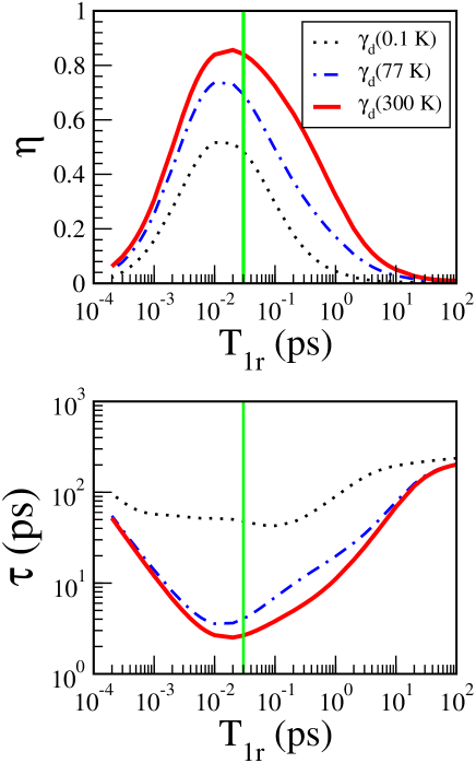
Figure 2: (Color online) Upper panel : efficiency computed at $t_{max}=5\ ps$, see Eq. (12), as a function of $T_{1r}$, for different dephasing rates, see Eq. (11). Lower panel: average transfer time, see Eq. (13), as a function of $T_{1r}$, for the same effective temperatures. ST has been indicated as a green vertical line. The initial condition is $\rho(0)=(1/2)(|1\rangle\langle 1|+|6\rangle\langle 6|)$.

The coupling to the RC also induces a shift of the energy of site $3$ (not only a decay width) kaplan . This shift is assumed to be generically of the form $\delta=\epsilon/T_{1r}$, where $\epsilon$ depends on the details of the coupling. We checked that the effect of changing $\epsilon$ randomly, so as to produce up to a $50\%$ change in the average level spacing, merely changes the efficiency at most by a few percent.

IV.2 Efficiency of energy transport in the presence of a finite temperature thermal bath

In this subection, we consider the effects of energy transport to the RC taking into consideration the interaction with a phonon bath at finite temperature, $T$, as described in Ref. qwalk . Here we consider that only site $3$ is coupled to the RC, as described above. The Lindblad-type master equation has the form

$$\frac{d\rho_{i,j}}{dt}=-\frac{i}{\hbar}\left(H_{\mathrm{eff}}\rho-\rho H_{\mathrm{eff}}^{+}\right)_{i,j}+L_{p}(\rho)_{ij},$$ (14)

where the action of the Lindblad operator on $\rho$, $L_{p}(\rho)$, is described in Eq. (5) of Ref. qwalk . With this choice, at sufficiently large time, the transition to the Gibbs distribution occurs, in absence of any other dissipative mechanism, such as the presence of “sinks”.

In Fig. 3 (upper panel), we present our results on the dependence of efficiency, $\eta$, as a function of $T_{1r}$, for three bath temperatures. As one can see, at the ST, indicated as a vertical green line, the efficiency is about $0.92$, and it weakly depends on temperature. We also mention that the maximal efficiency occurs near the ST.

The value of $T_{1r}$ at which one gets the maximal efficiency should not be confused with the average transfer time, see Eq. (13). In particular, in Fig. 3 lower panel, for parameters corresponding to the ST and room temperature, $T_{1r}\approx 30\ fs$ and $\tau\approx 2.1\ ps$.

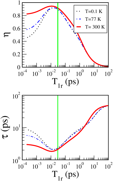
Figure 3: (Color online) Upper panel : efficiency computed at $t_{max}=5\ ps$, see Eq. (12), as a function of $T_{1r}$, for different temperatures of the phonon bath. Lower panel: average transfer time, see Eq. (13), as a function of $T_{1r}$, for the same temperatures. ST has been indicated as a green vertical line. The initial condition is $\rho(0)=(1/2)(|1\rangle\langle 1|+|6\rangle\langle 6|)$. We use as cut-off frequency of the spectral density of the thermal bath $\omega_{c}=150\ (cm)^{-1}$, and a reorganization energy $E_{R}=35(cm)^{-1}$, where the latter two quantities have been defined in Ref. qwalk .

Comparing Fig. 2 and 3, (upper panels), one can see that the presence of the phonon bath significantly increases the efficiency of energy transport to the RC, almost without changing the position of its maximum. We also would like to mention that in the presence of the thermal bath, the temperature effects on the efficiency are less significant than in presence of a classical noise, as in Fig. 2. Indeed dissipation helps the system to reach the site $3$ which has the lowest energy.

The analysis of this Section shows that the consequences of the ST are very important even in presence of dephasing and dissipation. For both models of thermal bath considered in this Section, the ST provides the maximal efficiency of energy transport. In the following we will consider only the model of the phonon bath presented in Sec. (IV.1), which, as shown in this Section, is sufficient to capture the main effects due to the phonon bath.

V Quantum vs. classical

ST implies the presence of a maximum of the energy transport efficiency as a function of the coupling time to the RC, $T_{1r}$. This effect is counter-intuitive from a classical point of view. Indeed, the probability to escape (decay to the RC) for a classical particle does not decrease as the escape rate ($1/T_{1r}$ from site $3$) is increased. In order to demonstrate the difference between the effects of quantum coherence on energy transfer discussed above, and the corresponding classical energy transport, we consider a classical master equation for the population dynamics, as in the Forster approach forster :

$$\frac{dP_{i}}{dt}=\sum_{k}(T_{i,k}P_{k}-T_{k,i}P_{i})-\frac{P_{i}}{T_{1}}-\delta_{i,3}\frac{P_{i}}{T_{1r}},$$ (15)

where $P_{i}$ is the probability to be on site $i$, $T_{i,k}$ is the transition matrix and the last two terms take into account the possibility for the classical excitation to escape the system. The transition rates from site $i$ to site $k$ have been computed from leegwater , neglecting the dependence on the coupling to the RC (for a classical particle, the probability to go from any site to site $3$ does not depend on the coupling to the RC).

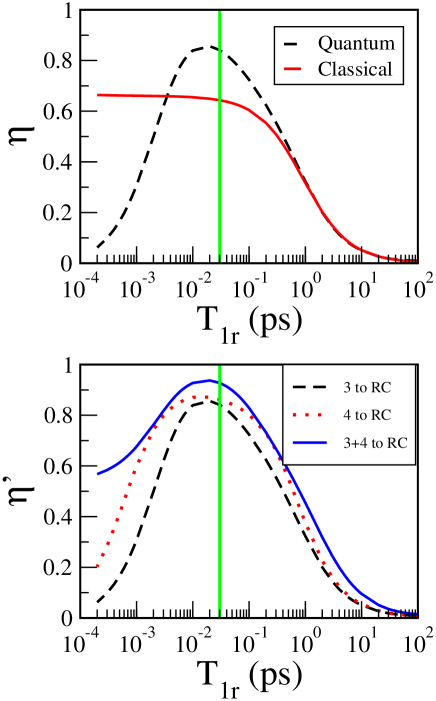
Figure 4: (Color online) Upper panel : quantum and classical efficiency computed at $t_{max}=5\ ps$, as a function of $T_{1r}$ at room temperature dephasing rate, $\gamma_{d}(T=300\,K)$, see Eq. (11). Lower panel: efficiency computed at $t_{max}=5\ ps$, using Eq. (16), as a function of $T_{1r}$ , at room temperature dephasing rate, $\gamma_{d}(T=300\,K)$, for different coupling to RC. The vertical green line represents ST. As initial conditions we choose $\rho(0)=(1/2)(|1\rangle\langle 1|+|6\rangle\langle 6|)$.

The comparison between classical and quantum behavior is shown in Fig. 4 (upper panel). The classical dynamics leads to a very different dependence of the efficiency on $T_{1r}$. Namely, the efficiency in the classical case does not exhibit a maximum but simply decays with $T_{1r}$. This shows that the ST effect is due to quantum coherence only.

VI Different coupling schemes

So far, we have considered the site $3$ to be the only one coupled to the RC. However, it is not known for sure which sites are connected to the RC, even though sites $3$ and $4$ are the most likely candidates, since they are closest to the RC lloyd . As mentioned above, the non-Hermitian Hamiltonian formalism easily allows one to describe different coupling schemes, which can be included in the effective Hamiltonian (4) by properly choosing the coupling transition amplitude, $A_{i}^{{}^{RC}}$, between the sites of the FMO complex and the RC. Note that while in the previous Section we indicated the channel in the RC with the number 3, here we label it as RC.

VI.1 Coupling from site 3 and 4

Since, to the best of our knowledge, it is not exactly known from experimental data how the energy transport occurs, in the following we choose three different situations, showing that the essential features of the phenomenon indicated in the previous Section does not change too much. Specifically we consider:

• only site 3 is coupled to RC, so that we set $A_{3}^{{}^{RC}}=\sqrt{\hbar/2T_{1r}}$ (as done above),

• only site 4 is coupled to the RC, so we set $A_{4}^{{}^{RC}}=\sqrt{\hbar/2T_{1r}}$,

• both sites $3$ and 4 are coupled to the RC, so we set $A_{3}^{{}^{RC}}=A_{4}^{{}^{RC}}=\sqrt{\hbar/2T_{1r}}$ .

In a general setting the probability for the excitation to be in the RC at time $t_{max}=5\ ps$ cannot be computed using Eq. (12), since by merely summing that expression for each site connected to the RC, we neglect interference effects. The efficiency should be computed using

$$\eta^{\prime}(t_{max})=1-Tr(\rho(t_{max}))-\frac{1}{T_{1}}\int_{0}^{t_{max}}\,dt\,Tr(\rho(t)).$$ (16)

Here, $1-Tr(\rho(t_{max}))$ is the probability that the excitation leaves the system by the time $t_{max}$. The last term in Eq. (16) is the probability that the excitation has been lost by recombination during this time. If there is just one site coupled to the RC, then Eq. (16) reduces to Eq. (12).
In Fig. 4 (lower panel) we show that the efficiency is sensitive to different coupling schemes. In particular, we notice that coupling through site $4$ achieves a greater efficiency than coupling through site $3$. If both sites are coupled to the RC, then the efficiency is further improved, and the decay for small coupling times is smaller than that for a single coupled site.

VI.2 Efficiency vs position of the RC

In the following, we consider a more realistic coupling scheme to RC, namely the case in which all sites of the FMO system have an electric dipole coupling to the same channel in the RC. This assumption can be justified since in the RC there are the same bacteriochlorophyll (BChl) molecules which compose the FMO system. So, it is reasonable to assume that the excitation is transferred to the RC by the same mechanism that operates between the BChl molecules in the FMO system.

The electric dipole transition amplitude from site $i$ to the RC can be written as:

$$V_{i}^{{}^{RC}}=\frac{C}{R_{{}_{i,RC}}^{3}}\left[\vec{\mu}_{i}\cdot\vec{\mu}_{{}_{RC}}-3(\vec{\mu}_{i}\cdot\hat{R}_{{}_{i,RC}})(\vec{\mu}_{{}_{RC}}\cdot\hat{R}_{{}_{i,RC}})\right],$$ (17)

where $R_{{}_{i,RC}}$ is the distance from site $i$ to the RC, ${\mu}_{i}$ is the dipole moment at the site $i$, and ${\mu}_{{}_{RC}}$ is the dipole moment assigned to the RC. We take the position of the BChls and their dipole moments from mohseni . Here, we assume that the coupling strength between the sites and the RC is equal to that between the sites, so that: $C|\mu|^{2}=134000$ $cm^{-1}(\AA)^{3}$, as in Ref. mohseni .

In order to determine the coupling amplitude from site $i$ to the continuum of states in the RC we evaluate the transfer rate, $\kappa_{i}$ from the Fermi-golden rule qwalk :

$$\kappa_{i}=\frac{2\pi\rho_{{}_{RC}}|V_{i}^{{}^{RC}}|^{2}}{\hbar},$$ (18)

where $\rho_{{}_{RC}}$ represents the density of states in the RC. It is interesting to observe that an expression for the transfer rate similar to (18) can be also obtained without perturbation theory, see for instance Ref. rotter3 , where the continuum was modeled as a semi-infinite lead. We can now determine the non-Hermitian Hamiltonian, Eq. (4), setting:

$$A_{i}^{{}^{RC}}=\sqrt{2\pi\rho_{{}_{RC}}}\ V_{i}^{{}^{RC}}.$$

Note that now the coupling between the FMO complex and the RC depends on the position of the RC. In order to determine how the efficiency of energy transfer depends on the position of the RC w.r.t. the FMO complex, we assume ${{\vec{\mu}}}_{{}_{RC}}={\vec{\mu}}_{3}$ and place the RC in the same $y$ and $z$ position of site $3$, as given in mohseni . The transport efficiency has been studied by varying the distance, $d$, from the site $3$ along the $x$ direction. In order to compute the transition amplitude, $A_{i}^{{}^{RC}}$, we need the density of states of the RC which, to the best of our knowledge is not known experimentally. For this reason we consider different densities of states, respectively larger, equal or smaller than the density of states of the FMO system, $\rho_{{}_{FMO}}\simeq 1/D$, $D$ being the mean level spacing of the FMO complex discussed in Sec. (III).

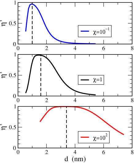
Figure 5: (Color online) Efficiency, Eq. (16), computed at $t_{max}=5\ ps$ vs the distance $d$ ($nm$) of the RC from site $3$ in the FMO complex for different ratios $\chi=\rho_{{}_{RC}}/\rho_{{}_{FMO}}$. Here, an electric dipole coupling between the RC and the FMO system, see Eq. (17), has been considered. The vertical dashed lines, obtained from Eq. (19), represent the critical distances at which superradiance transition occurs. As initial conditions we choose $\rho(0)=(1/2)(|1\rangle\langle 1|+|6\rangle\langle 6|)$. Data in this figure refer to a room temperature dephasing rate, $\gamma_{d}(T=300\,K)$, see Eq. (11).

We show in Fig. (5) how the efficiency, computed with Eq. (16) using Eq. (10), varies as a function of the distance from the RC to site $3$ of the FMO system. In Fig. (5) we consider a room temperature dephasing rate $\gamma_{d}(T=300\ K)$, for different ratios, $\chi=\rho_{{}_{RC}}/\rho_{{}_{FMO}}=0.1,1,10^{2}$, respectively, from the upper to the lower panel. As one can see, the optimal distance, which is the distance that maximizes the efficiency, slowly depends on the density of states in the RC.

We can use the superradiant criterium obtained in Eq. (7) to get an analytical expression for the optimal distance of the RC from the FMO complex. Since site $3$ is the closest to the RC, we can use Eq. (7) and we find that the ST occurs for $\hbar\kappa_{3}=D$. Finally, from Eq. (18) we have:

$$d_{max}=(2\pi B^{2})^{\frac{1}{6}}(\rho_{{}_{RC}}\rho_{{}_{FMO}})^{\frac{1}{6}},$$ (19)

where,

$$B=C\left[\vec{\mu}_{3}\cdot\vec{\mu}_{{}_{RC}}-3(\vec{\mu}_{3}\cdot\hat{R}_{{}_{3,RC}})(\vec{\mu}_{{}_{RC}}\cdot\hat{R}_{{}_{3,RC}})\right],$$ (20)

see Eq. (17). Eq. (19) gives us the distance at which superradiance transition occurs. The critical distance obtained from Eq. (19) is shown in Fig. (5) as dashed vertical lines. As one can see, the estimate is very good. Note that changing the density of states in the RC from $\rho_{{}_{FMO}}/10$ to $10^{2}\rho_{{}_{FMO}}$ only changes the optimal distance from $1\ nm$ to $3\ nm$. These distances are consistent with available structural data for the RC-FMO complex, see for instance rc . The result is remarkable since it shows that the superradiant criterium suffices to determine the optimal distance from the RC to the FMO complex for a wide range of values for the density of states of the RC.

VII Conclusion

We have analyzed energy transport in the FMO system with the aid of a non-Hermitian Hamiltonian approach. This allows us to take into account the effect of the coupling of the FMO system to the reaction center in a consistent way, not merely phenomenologically, as is usually done in the literature. We have shown that by increasing the strength of the coupling to the reaction center, a superradiance transition occurs. This transition occurs at approximately the same value of the coupling for which energy transport efficiency is maximal. Indeed, the superradiance transition is due to coherent constructive interference between the paths to the RC, and this effect enhances the rate of energy transfer. Since the ST effect is due to quantum coherence, one might expect that any consequences of ST would disappear in the presence of dephasing and relaxation provided by the thermal bath. On the contrary, we have shown that the effect of superradiance survives in the presence of the thermal bath, and the maximal efficiency only depends weakly on temperature. We have also estimated the ST critical value analytically. For coupling strengths of the FMO system to the RC near the critical one, where the superradiance transition takes place, we obtained average energy transfer times comparable to experimental values (a few picoseconds). Finally, we took into account a realistic coupling scheme between the FMO system and the RC, and derived from the superradiance condition the analytical expression, Eq. (19), for the optimal distance from the RC to the FMO complex. This analytical expression depends on the density of states in the RC. Within a wide range of density of states the optimal distance which we obtained analytically is approximately a few nanometers and is consistent with available structural data on RC. Note also that Eq. (19) is valid for a generic Donor-Acceptor complex.

Our analysis shows that the superradiance mechanism might play an important role in explaining the efficiency of quantum transport in photosynthetic light-harvesting systems and in engineering artificial light harvesting systems.

Acknowledgments. This work has been supported by Regione Lombardia and CILEA Consortium through a LISA (Laboratory for Interdisciplinary Advanced Simulation) Initiative (2010/11) grant [link:http://lisa.cilea.it]. Support from grant D.2.2 (2010) from Università Cattolica is also acknowledged. The work by GPB was carried out under the auspices of the National Nuclear Security Administration of the U.S. Department of Energy at the Los Alamos National Laboratory under Contract No. DE-AC52- 06NA25396. MM has been supported by the NSERC Discovery Grant No. 205247. F.B., M.M. and G.P.B thank the Institut Henri Poincare (IHP) for partial support at the final stage of this work.

References

- (1) G.S. Engel et al., Nature 446, 782 (2007).
- (2) G. Panitchayangkoon et al., PNAS 107, 12766 (2010).
- (3) M. Sarovar, A. Ishizaki, G.R.Fleming and K.B.Whaley, Nature Physics 6, 462 (2010).
- (4) H. Hossein-Nejad and G. D. Scholes, New J. Phys. 12, 065045 (2010).
- (5) M. Mohseni, P. Rebentrost, S. Lloyd and A. Aspuru-Guzik, J. Chem. Phys. 129, 174106 (2008).
- (6) S. Lloyd and M. Mohseni, New J. Phys. 12, 075020 (2010).
- (7) G. D. Scholes, Chem. Phys. 275, 373 (2002).
- (8) R. H. Dicke, Phys. Rev. 93, 99 (1954).
- (9) V. V. Sokolov and V. G. Zelevinsky, Nucl. Phys. A504, 562 (1989); Phys. Lett. B 202, 10 (1988); I. Rotter, Rep. Prog. Phys. 54, 635 (1991).
- (10) V. V. Sokolov and V. G. Zelevinsky, Ann. Phys. (N.Y.) 216, 323 (1992).
- (11) M. Pudlak, K. N. Pichugin, R. G. Nazmitdinov and R. Pincak, Phys. Rev. E 84, 051912 (2011).
- (12) J. J. M. Verbaarschot, H. A. Weidenmüller, and M. R. Zirnbauer, Phys. Rep. 129, 367 (1985); N. Lehmann, D. Saher, V. V. Sokolov, and H.-J. Sommers, Nucl. Phys. A582, 223 (1995); Y. V. Fyodorov and H.-J. Sommers, J. Math. Phys. 38, 1918 (1997); H.-J. Sommers, Y. V. Fyodorov, and M. Titov, J. Phys. A: Math. Gen. 32, L77 (1999).
- (13) G. L. Celardo, F. M. Izrailev, V. G. Zelevinsky, and G. P. Berman, Phys. Lett B 659, 170 (2008); G. L. Celardo, F. M. Izrailev, V. G. Zelevinsky, and G. P. Berman, Phys. Rev. E, 76, 031119 (2007); G. L. Celardo, S. Sorathia, F. M. Izrailev, V. G. Zelevinsky, and G. P. Berman, CP995, Nuclei and Mesoscopic Physics - WNMP 2007, ed. P. Danielewicz, P. Piecuch, and V. Zelevinsky.
- (14) A. Volya and V. Zelevinsky, Phys. Rev. C 67, 054322 (2003); Phys. Rev. Lett. 94, 052501 (2005); Phys. Rev. C 74, 064314 (2006).
- (15) H.-J. Stöckmann, E. Persson, Y.-H. Kim, M. Barth, U. Kuhl, and I. Rotter, Phys. Rev. E 65, 066211 (2002); R. G. Nazmitdinov, H.-S. Sim, H. Schomerus, and I. Rotter, Phys. Rev. B 66, 241302 (2002).
- (16) G.L. Celardo and L. Kaplan, Phys. Rev. B 79, 155108 (2009); G. L. Celardo, A. M. Smith, S. Sorathia, V. G. Zelevinsky, R. A. Sen’kov, and L. Kaplan, Phys. Rev. B 82, 165437 (2010).
- (17) A. F. Sadreev and I. Rotter, J. Phys. A 36, 11413 (2003).
- (18) N. Renaud, M. A. Ratner, and V. Mujica J. Chem. Phys. 135, 075102 (2011).
- (19) C. Mahaux and H. A. Weidenmüller, Shell Model Approach to Nuclear Reactions (North Holland, Amsterdam, 1969).
- (20) M. Mohseni, A. Shabani, S. Lloyd, H. Rabitz, arXiv:1104.4812v1 [quant-ph]; A. Shabani, M. Mohseni, H. Rabitz, S. Lloyd, arXiv:1103.3823v3 [quant-ph].
- (21) Recent studies reported the presence of an additional Bchl pigment per subunit: A. Ben-Shem, F. Frolow and N. Nelson, FEBS Lett. 2004, 564, 274 (2004); D.E. Tronrud, J. Z. Wen, L. Gay, R. E. Blankenship, Photosynth. Res. 100, 79 (2009). These new findings do not change the main conclusions of our analysis.
- (22) P.W. Milonni and P.L. Knight, Phys. Rev. A 10, 1096 (2009).
- (23) A. Messiah, Quantum Mechanics (North Holland Publishing company, Amsterdam 1962) English ed. Vol II, Chapter .
- (24) P. Rebentrost, M. Mohseni, I.Kassal, S. Lloyd and A. Aspuru-Guzik, New J. Phys. 11, 033003 (2009); P. Rebentrost, M. Mohseni and A. Aspuru-Guzik A, J. Phys. Chem. B 113, 9942 (2009).
- (25) M. B. Plenio and S. F. Huelga, New J. Phys. 10, 113019 (2008); F. Caruso, A. W. Chin, A. Datta, S. F. Huelga and M. B. Plenio, J. Chem. Phys. 131, 105106 (2009).
- (26) F.M. Izrailev, A.A. Krokhin and N.M. Makarov, Phys. Rep. 512, 125 (2012).
- (27) P. W. Anderson, Phys. Rev. 109, 1492 (1958).
- (28) Th. Forster, In Modern Quantum Chemistry, Sinannouglu, O., Ed.; Acad. Press: New York, (1965) p. 93.
- (29) J.A. Leegwater, J. Phys. Chem. 100, 14403 (1996).
- (30) A. F. Sadreev and I. Rotter, J. Phys. A 36, 11413 (2003).
- (31) H.-W. Remigy et al., J. Mol. Biol. 290, 851(1999); H.-W. Remigy et all., Photosynthesis Res. 71, 91 (2002).