Mechanical cat states in graphene resonators

Abstract

We study the quantum dynamics of a symmetric nanomechanical graphene resonator with degenerate flexural modes. Applying voltage pulses to two back gates, flexural vibrations of the membrane can be selectively actuated and manipulated. For graphene, nonlinear response becomes important already for amplitudes comparable to the magnitude of zero point fluctuations. We show, using analytical and numerical methods, that this allows for creation of cat-like superpositions of coherent states as well as superpositions of coherent cat-like non-product states.

Coherent superposition of states are characteristic traits of quantum mechanics. These phenomena have already been realized in many-particle contexts such as trapped ultra-cold atoms Monroe_1996 , superconductors Friedman_2000 and photonic systems Haroche_2008 . A current challenge is to observe these effects for collective degrees of freedom in a macroscopic context in, e.g., mechanical resonators Schwab_2005 .

Recent advances in cooling mechanical resonators and sensitive displacement detection have allowed reaching the motional ground state and observing zero point fluctuations of center of mass Cleland_2010 ; Lehnert_2011 . Active manipulation and characterization of the quantum state of these systems, as already achieved with photons Cleland_2009 , seem to be within reach. For a mechanical system, a desirable state to generate is a ’cat’ state. This is a coherent superposition of two minimum uncertainty wave packets separated by more than their individual quantum fluctuations.

For the harmonic oscillator a minimum uncertainty wave packet is a coherent state $\left|\alpha\right>=\exp[\alpha a^{{\dagger}}-\alpha^{\ast}a]|0\rangle$ generated by displacing the oscillator ground state Gardiner_book . As shown by Yurke and Stoler Yurke_Stoler , for a nonlinear oscillator $H=\hbar\omega_{0}\hat{n}+\hbar\Omega\hat{n}^{2}$ an initial coherent state $\left|\alpha\right>$ will after a time $t=\pi/(2\Omega)$ evolve into the cat state $(1/\sqrt{2})\left[e^{-i\pi/4}\left|\alpha\right>+e^{i\pi/4}\left|-\alpha\right>\right]$ with the maximum spatial separation $\Delta=2|\alpha|$.

Nanoelectromechanical resonators are typically intrinsically nonlinear Cleland_book . The amplitudes needed to observe nonlinear effects are often orders of magnitude larger than the quantum zero point fluctuations $x_{0}=\sqrt{\hbar/m\omega_{0}}$. A cat state obtained due to this nonlinearity would have a separation $\Delta\gg x_{0}$. As the decoherence rate scales as $(\Delta/x_{0})^{2}$ Holmes_1986 ; Kartner_1993 this has, until now, been unfeasible. Instead, coupling to auxillary quantum systems has been proposed to engineer the nonlinearity Jacobs_2007 ; Milburn_2009 .

We show how the intrinsic nonlinearity in a graphene membrane resonator can be used to prepare cat states by applying voltage pulses to local backgates. The reason for using graphene is the ultra-low mass of the graphene sheet which leads to a large $x_{0}$, and an onset of nonlinear response at small amplitudes Atalaya_2008 ; Bachtold_2011 . This implies that cat states with moderate ratios $(\Delta/x_{0})$ can be constructed without the need for engineered auxillary quantum systems or feedback loops. Another feature of two-dimensional mechanical resonators is that they can be designed to have degenerate flexural modes. Coupling between these modes can be controlled by external perturbations such as gate electrodes, which can be utilized for state manipulation.

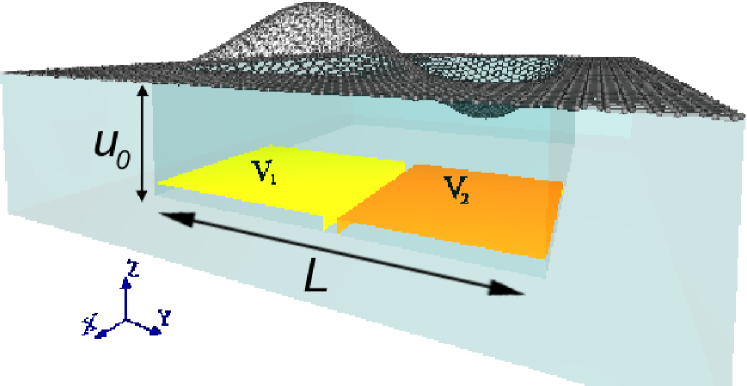
Figure 1: (Color online) Cross section of a square graphene membrane resonator. A fully clamped graphene membrane with side $L$ is suspended a distance $u_{0}$ above the substrate. Below, covering two adjacent quadrants beneath the membrane, are local backgates with time dependent voltage biases $V_{1,2}(t)$. By applying pulses to the local gates, cat-like superpositions of flexural mode states, as well as superpositions of coherent cat-like non-product states, can be generated.

For concreteness we consider a square graphene membrane with mass density $\rho_{0}=7.6\cdot 10^{-7}$ kg/m² and side length $L$. The sheet is suspended in the $xy$-plane at a distance $u_{0}$ above two local backgates (see Fig. 1). They cover adjacent quadrants below the membrane and are have voltages $V_{1}(t)$ and $V_{2}(t)$. The Hamiltonian density of the system can be divided into two parts: $\mathscr{H}=\mathscr{H}_{0}({\bf x})+\mathscr{H}_{G}({\bf x},V_{1},V_{2})$, where ${\bf x}\equiv(x,y)$. Here $\mathscr{H}_{0}({\bf x})$ gives the intrinsic mechanics of the membrane while the coupling to the gates is described in $\mathscr{H}_{G}({\bf x},V_{1},V_{2})$. To a first approximation one finds Atalaya_2008 ; Daniel_book

$$\mathscr{H}_{0} = \frac{\pi_{0}^{2}}{2\rho_{0}}+\frac{T_{0}}{2}\big{|}\nabla u\big{|}^{2}+\frac{T_{1}}{4}\big{|}\nabla u\big{|}^{4}$$ (1)

where $u({\bf x},t)$ is the out of plane displacement and $\pi_{0}$ its conjugate momentum density. The built-in tension is $T_{0}$ and the stretching-induced tension is determined by $T_{1}=(\mu+\lambda/2)$ where the Lamé-parameters of graphene are $\mu\approx 3\lambda\approx 9$ eV/Ų Yakobsson_2001 . We model $\mathscr{H}_{G}$ in the local approximation as $\mathscr{H}_{G}={\epsilon_{0}V({\bf x},t)^{2}}/[{u_{0}+u({\bf x})]}$, where $\epsilon_{0}=8.854\cdot 10^{-12}$ F/m and $V({\bf x},t)$ is the local gate potential. Expanding $u$ and $\pi_{0}$ in mode functions as

$$u=\sum_{\bf{k}}q_{\bf{k}}(t)\varphi_{\bf{k}}({\bf{x}}),\,\,\,\pi_{0}=\displaystyle{\frac{1}{L^{2}}}\sum_{\bf{k}}p_{\bf{k}}(t)\varphi_{\bf{k}}({\bf{x}}),$$

using $\varphi_{\bf{k}}=2\sin(k_{x}x)\sin(k_{y}y)$ and ${\bf k}=(k_{x},k_{y})=(n,m)\pi/L$ for $n,m=1,2,...$, gives $H=H_{0}+H_{G}$ with

$$H_{0}=\sum_{\bf{k}}\frac{1}{2M}\Big{(}p_{\bf{k}}^{2}+M^{2}\omega_{\bf{k}}^{2}q_{\bf{k}}^{2}\Big{)}+\frac{1}{2}\sum_{\bf{kk^{{}^{\prime}}}}F_{\bf{kk^{{}^{\prime}}}}(q_{\bf{k}}q_{\bf{k^{{}^{\prime}}}})^{2},$$

$$H_{G}=K_{0}+\sum_{\bf{k}}K_{\bf{k}}q_{\bf{k}}+\frac{1}{2}\sum_{\bf{kk^{{}^{\prime}}}}K_{\bf{kk^{{}^{\prime}}}}q_{\bf{k}}q_{\bf{k^{{}^{\prime}}}}.$$

Here $M=\rho_{0}L^{2}$ and $\omega_{\bf k}=({T_{0}}/{\rho_{0}})^{\frac{1}{2}}\bf|{k}|$. The coefficients $F_{\bf{kk^{{}^{\prime}}}}$ and $K_{\bf{kk^{{}^{\prime}}}}$ will be discussed below.

We restrict attention to the two lowest degenerate modes with ${\bf{k}}_{1}=(\pi/L,2\pi/L)$, and ${\bf{k}}_{2}=(2\pi/L,\pi/L)$ and their frequencies $\omega_{1,2}=(\pi/L)\sqrt{5T_{0}/\rho_{0}}$. We label these modes ${\bf 1}$ and ${\bf 2}$. Quantizing, by imposing the commutation relation $[\hat{q}_{\bf{k}},\hat{p}_{\bf{k^{\prime}}}]=i\hbar\delta_{\bf k,\bf k^{\prime}}$, yields

$$H=\frac{\hat{p}_{1}^{2}+\hat{p}_{2}^{2}}{2M}+\frac{M\omega_{1}^{2}}{2}(\hat{q}_{1}^{2}+\hat{q}_{2}^{2})+D(\hat{q}_{1}^{4}+\hat{q}_{2}^{4})+F\hat{q}_{1}^{2}\hat{q}_{2}^{2}$$

$$+K_{1}\hat{q}_{1}+K_{2}\hat{q}_{2}+K_{12}\hat{q}_{1}\hat{q}_{2}+S_{1}\hat{q}_{1}^{2}+S_{2}\hat{q}_{2}^{2}.$$ (2)

Introducing $\kappa\equiv{\epsilon_{0}L^{2}}/{u_{0}^{2}\pi^{2}}$ the coefficients in (2) are

$$D\equiv\frac{161\pi^{4}T_{1}}{4L^{2}},\,\,F\equiv\frac{41\pi^{4}T_{1}}{2L^{2}},\,\,K_{1,2}=\kappa(V_{1}^{2}\mp V_{2}^{2}),$$

$$K_{12}=-\frac{16\kappa}{9u_{0}}(V_{1}^{2}-V_{2}^{2}),\,\,S_{1,2}=-{\kappa\pi^{2}V_{1,2}^{2}}/{8u_{0}}$$ (3)

For time dependent $V_{1,2}(t)$ the Hamiltonian (2) describes the excitation and evolution of two (nearly) degenerate interacting flexural modes. Also other modes, not included in  (2), will be excited by the gates. This two-mode approximation is valid for weak intermode interaction and when the other modes are off resonance with the modes ${\bf 1}$ and ${\bf 2}$.

For cat state generation we analyze the evolution of the system, initially in the ground state, subject to a common bias pulse on the two gates, i.e., $V_{1}=V_{2}=V_{0}\theta(t)$ where $\theta(t)$ is the unit step function. Then (2) reduces to

$$H=\hbar\sum_{j=1,2}\omega[\hat{a}_{j}^{\dagger}\hat{a}_{j}+\frac{\varepsilon}{4}(\hat{a}_{j}+\hat{a}_{j}^{\dagger})^{4}]+\hbar\omega\delta(t)(\hat{a}_{2}+\hat{a}_{2}^{\dagger})+H_{12},$$ (4)

where $\omega^{2}\equiv\omega_{1,2}^{2}+2S_{1,2}/M$, $H_{12}=F\hat{q}_{1}^{2}\hat{q}_{2}^{2}$, $\varepsilon={D\hbar}/{M^{2}\omega^{3}}$, and $\delta(t)={\sqrt{2}\kappa V_{0}^{2}}/{\sqrt{\hbar M\omega^{3}}}$. The $\hat{a}_{j}^{(\dagger)}$ are defined through $\hat{p}_{j}=ip_{0}(\hat{a}_{j}^{{\dagger}}-\hat{a}_{j})/\sqrt{2}$, and $\hat{q}_{j}=x_{0}(\hat{a}_{j}^{{\dagger}}+\hat{a}_{j})/\sqrt{2}$ with $x_{0}\equiv\sqrt{\hbar/M\omega}$ and $p_{0}\equiv\sqrt{M\hbar\omega}$.

We consider the situation when the system is cooled to $k_{B}T\ll\hbar\omega$ and at time $t=0$ the flexural modes are in their ground states $\left|0\right>$. Equal voltage pulses are applied to both gates $\delta(t)=\delta_{0}\theta(t)$, inducing system’s evolution. As mode ${\bf 1}$ will not be appreciably affected by the weak coupling term $H_{12}$, the dynamics of the modes decouple. Hence, mode ${\bf 1}$ will remain close to its ground state for $t>0$. The remaining mode ${\bf 2}$ describes a particle in a potential $v(\xi)=\sqrt{2}\delta_{0}\xi+\xi^{2}/2+\epsilon\xi^{4}$ with $\xi=q_{2}/x_{0}$ and an equilibrium position $\xi_{0}$. Introducing the displaced oscillator operator $b_{2}=a_{2}-\xi_{0}/\sqrt{2}$, and applying the rotating wave approximation (RWA), the Hamiltonian becomes $H=\hbar\tilde{\omega}\hat{n}_{b}+3\hbar\omega\varepsilon\hat{n}_{b}^{2}/2,$ where

$$\hat{n}_{b}=\hat{b}^{{\dagger}}_{2}\hat{b}_{2},\>\>\>\>\tilde{\omega}=\omega[1+3\varepsilon(1/2+2\xi_{0}^{2})].$$ (5)

If $\epsilon\xi_{0}^{2}\ll 1$, the situation is similar to the one in Yurke_Stoler . The intial state $\left|\psi(t=0)\right>=\left|0\right>_{a_{2}}$ resembles a coherent state in the $b_{2}$-basis, i.e, $\left|0\right>_{a_{2}}\approx\left|-\xi_{0}/\sqrt{2}\right>_{b_{2}}$. If the system evolves a time $T_{1}=\pi/(3\omega\varepsilon)$, we expect to find the state

$$|\psi(T_{1})\rangle\propto e^{-i\pi/4}|-\xi_{0}e^{-i\tilde{\omega}t}/\sqrt{2}\rangle_{b_{2}}+e^{i\pi/4}|\xi_{0}e^{-i\tilde{\omega}t}/\sqrt{2}\rangle_{b_{2}}$$

which, to an overall phase, is in $a$-basis given by

$$|\psi(T_{1})\rangle\propto|\xi_{0}(1-e^{-i\tilde{\omega}t})/\sqrt{2}\rangle_{a_{2}}+i|\xi_{0}(1+e^{-i\tilde{\omega}t})/\sqrt{2}\rangle_{a_{2}}.$$ (6)

To verify this we simulated the dynamics using the full two-mode Hamiltonian in  (2) and a Hilbert space of $40^{2}$ number states in the occupation basis. The parameters used were $L=126$ nm, $u_{0}=60$ nm, $T_{0}=0.003$ N/m, and $V_{0}=0.23$ V. This corresponds to $\omega/(2\pi)\approx 560$ MHz, $\varepsilon=7\cdot 10^{-4}$ and $\delta_{0}=1.3$. The position shift becomes $\xi_{0}\approx-1.8\approx-\sqrt{2}\delta_{0}$.

In Fig. 2a the probability density of finding mode ${\bf 2}$ at a position $\xi$ is shown as function of time. Only instants where $t=2\pi n/\tilde{\omega}$ are sampled hence fast oscillations with frequency $\omega$ are not visible. The initial state $\left|0\right>_{a_{2}}=\left|-\xi_{0}/\sqrt{2}\right>_{b_{2}}$ evolves into a first cat-like state at time $T_{1}\approx 0.42$ $\mu$s $\approx\pi/(3\omega\varepsilon)$. This and the following cat-like state emerging at $T_{2}\approx 1.27$ $\mu$s  $\approx\pi/(\omega\varepsilon)$ are marked with vertical dashed lines. The simulations also verified that mode ${\bf 1}$ remains close to its ground state.

To read out the state the two gates may form part of a capacitor in an LC-circuit with $\omega_{\rm LC}\gg\omega$ in the resolved sideband limit. This allows for side band cooling and measurement of the quadrature operator Hertzberg_2009 $X_{\nu}=[e^{i\nu}a^{\dagger}_{2}+e^{-i\nu}a_{2}]/\sqrt{2}$. In Fig. 2b we show the envelopes of the average $\left<X_{\nu}\right>$ along with the quantum fluctuations $\left<\Delta X_{\nu}^{2}\right>$ as functions of time. The fluctuations have the form $\left<\Delta X_{\nu}^{2}\right>\sim A(t)+B(t)\cos(2\omega t)$, where $A$ and $B$ vary slowly in time. A signature of the built up cat state is the reduction of $\left<X_{\nu}\right>$ with an increase in $\left<\Delta X_{\nu}^{2}\right>$.

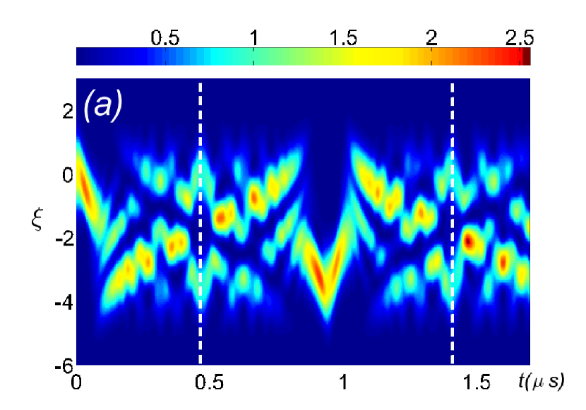
Figure 2: (Color online) (a) False color plots of snapshots of time evolution of the position probability distribution for one flexural mode. The snapshots are taken at the turning points of the corresponding classical trajectory of the system. The positions (y-axis) are scaled to the quantum zero point fluctuations $x_{0}$. with vertical, white dashed lines. (b) Corresponding time evolution of the envelopes of the quadrature $\left<X_{\nu}\right>$ (continous line) and its associated quantum fluctuations $\left<\Delta X_{\nu}^{2}\right>$; $A(t)$ (dashed line), $B(t)$ (dashdotted line). The appearance of a cat state is signalled by a decrease in $\left<X_{\nu}\right>$ along with an increased contribtion from quantum fluctuations $\left<\Delta X_{\nu}^{2}\right>$ in the noise of $\left<X_{\nu}\right>$. Vertical dashed lines indicate the agreement with Fig. 2a.

For the cat state to emerge, dissipation must be weak. Even at zero temperature damping will cause decoherence. As shown in Holmes_1986 ; Kartner_1993 this occurs on a time scale $t_{c}\sim Q/\omega\xi_{0}^{2}$ where $Q$ is the resonator quality factor. Requiring $t_{c}\gg T_{1}$ yields $Q\gg\xi_{0}^{2}/\varepsilon$. For our protoype system, this inequality is fulfilled if $Q>10^{4}$. Recently Q-factors up to $Q\sim 10^{5}$ were reported in graphene resonators Bachtold_2011 .

The cat state above is a product state between modes ${\bf 1}$ and ${\bf 2}$ in $a$-basis. We now demonstrate a cat-like state involving both modes that is not a product state in this basis. Preparing the system in the ground state $\left|0,0\right>_{a}$ and switching on only one gate at time $t=0$, i.e., $V_{2}=0$, $V_{1}=\tilde{V}$, the degeneracy is lifted. Just as the operators $a^{({\dagger})}_{j}$ and $b^{({\dagger})}_{j}$ respectively diagonalize the linear part of (2) when $V_{1,2}=0$ and $V_{1}=V_{2}\neq 0$, the normal modes when $V_{1}\neq V_{2}=0$ are found by diagonalizing the linear part of (2) by means of the transformation

$$d_{1}=\cos(\theta)a_{1}-\sin(\theta)a_{2},$$

$$d_{2}=\sin(\theta)a_{1}+\cos(\theta)a_{2}+\eta_{0}.$$

Here $\eta_{0}=\kappa\tilde{V}^{2}/\sqrt{\hbar M\omega^{3}}$ and we have neglected terms of order $|(\Omega_{1}-\Omega_{2})/\omega|\ll 1$, where $\Omega_{1,2}^{2}=\omega^{2}\mp K_{12}/M$ are the new eigenmode frequencies. The Hamiltonian (2) now transforms to

$$\tilde{H}=\hbar\sum_{j=1,2}\Omega_{j}d_{j}^{{\dagger}}d_{j}+\tilde{H}_{NL},$$ (7)

where $\tilde{H}_{NL}$ is quartic in $d$-operators. As parameters like length and tension are never exactly equal in both $x$ and $y$-directions, the two modes ${\bf 1,2}$ are only approximately degenerate, i.e. $\omega_{1}\neq\omega_{2}$. This leads to the requirement $|(\Omega_{1}-\Omega_{2})/(\omega_{1}-\omega_{2})|\gg 1$ so that $\theta\simeq\pi/4$, and

$$\tilde{H}_{NL} = \frac{\tilde{\varepsilon}}{4}(d_{1}+d_{1}^{{\dagger}})^{4}+\frac{\tilde{\varepsilon}}{4}(d_{2}+d_{2}^{{\dagger}}-2\eta_{0})^{4}+$$

$$\lambda(d_{1}+d_{1}^{{\dagger}})^{2}(d_{2}+d_{2}^{{\dagger}}-2\eta_{0})^{2},$$

$$\tilde{\varepsilon}={\hbar(2D-F)}/{4M^{2}\omega^{3}},\>\>\>\>\lambda={\hbar(6D-F)}/{2M^{2}\omega^{3}}.\\$$

The initial state $\left|0,0\right>_{a}$ is in $d$-basis $\left|0,\eta_{0}\right>_{d}$. After evolution with (7) this state will, analogous to the situation studied above, enter a superposition at time $\tilde{T}_{1}\approx\pi/(3\omega\tilde{\varepsilon})\approx 0.65\mu s$

$$|\psi(\tilde{T}_{1})\rangle \propto \left|0,\eta_{0}\right>_{d}+i\left|0,-\eta_{0}\right>_{d}+\alpha\left|\chi\right>.$$ (9)

Here $\alpha\left|\chi\right>=\alpha\sum_{n=1}\left|n\right>_{d_{1}}\left|\Psi_{n}\right>_{d_{2}}$ is due to the quartic coupling term in (Mechanical cat states in graphene resonators). The state component $\left|0,\eta_{0}\right>_{d}+i\left|0,-\eta_{0}\right>_{d}$ corresponds to a cat-like non-product state $\left|0,0\right>_{a}+i\left|-\sqrt{2}\eta_{0},-\sqrt{2}\eta_{0}\right>_{a}$ in $a$-basis.

To verify the creation of this state we numerically analyze the evolution of $|0,0\rangle_{a}$. Fig. 3a shows the Wigner distribution $W(\xi_{1},\pi_{1})=(2\pi)^{-1}\int d\xi~{}e^{-i\pi_{1}\xi}\langle\xi_{1}+\xi/2|\hat{\rho}_{1}|\xi_{1}-\xi/2\rangle$ of the reduced density matrix $\hat{\rho}_{1}$ of mode ${\bf 1}$ in $a$-basis at $\tilde{T}_{1}$. The distribution is plotted as function of the dimensionless position $\xi_{1}$ and momentum $\pi_{1}$ and has a bimodal structure. The distribution for mode ${\bf 2}$ is identical, $W(\xi_{2},\pi_{2})=W(\xi_{1},\pi_{1})$.

To remove $\alpha|\chi\rangle$ from (9) we introduce the projection operators $\hat{P}_{n}=\left(\left|n\right>\left<n\right|\right)_{d_{1}}\otimes\hat{I}_{d_{2}}$ and study (Fig. 3b) the Wigner distribution of the projection $\hat{P}_{0}|\psi(\tilde{T}_{1})\rangle$. One can here clearly recognize the distribution corresponding to the state $\left|0,0\right>_{a}+i\left|-\sqrt{2}\eta_{0},-\sqrt{2}\eta_{0}\right>_{a}$, which is displayed in Fig. 3c for reference. To ensure that the $\alpha|\chi\rangle$ component is not of major significance, the time evolution of the projections $\langle\hat{P}_{0}(t)\rangle$, $\langle\hat{P}_{2}(t)\rangle$ and $\langle\hat{I}-\hat{P}_{0}(t)-\hat{P}_{2}(t)\rangle$ are shown in Fig. 3d.

Figure 3: (Color online) (a) False color plot of reduced Wigner distribution of the time evolved initial state $|0,0\rangle_{a}$, sampled at $\tilde{T}_{1}$ as function of the dimensionless position $\xi_{1}$ and momentum $\pi_{1}$. The reduced Wigner distributions are identical for both modes $W(\xi_{1},\pi_{1})=W(\xi_{2},\pi_{2})$. A bimodal structure is seen. (b) False color plot of Wigner distribution of $\hat{P}_{0}\hat{\rho}_{1}(\xi_{1},\pi_{1},\tilde{T}_{1})\hat{P}_{0}$, clearly demonstrating bimodality. (c) False color plot of Wigner distribution of $\left|0,0\right>_{a}+i\left|-\sqrt{2}\eta_{0},-\sqrt{2}\eta_{0}\right>_{a}$. The similarity to the projection in (b) is evident. (d) Time evolution of projections $\langle\hat{P}_{0}(t)\rangle$, $\langle\hat{P}_{2}(t)\rangle$ and $\langle\hat{I}-\hat{P}_{0}(t)-\hat{P}_{2}(t)\rangle$. The most significant contribution comes from $\langle\hat{P}_{0}(t)\rangle$.

The expression for $|\psi(\tilde{T}_{1})\rangle$ in (9) is in RWA. In the Schrödinger picture the state has a fast oscillating component and is at $t=\tilde{T}_{1}$

$$|\psi(t)\rangle_{S}=|0,\>\eta_{0}e^{-i\tilde{\Omega}_{2}t}\rangle_{d}+i|0,-\eta_{0}e^{-i\tilde{\Omega}_{2}t}\rangle_{d}+\alpha|\chi\rangle$$

$$=\left|\frac{\eta_{0}}{\sqrt{2}}(e^{-i\tilde{\Omega}_{2}t}-1),\frac{\eta_{0}}{\sqrt{2}}(e^{-i\tilde{\Omega}_{2}t}-1)\right>_{a}$$

$$+i\left|-\frac{\eta_{0}}{\sqrt{2}}(e^{-i\tilde{\Omega}_{2}t}+1),-\frac{\eta_{0}}{\sqrt{2}}(e^{-i\tilde{\Omega}_{2}t}+1)\right>_{a}+\alpha|\chi\rangle.$$

Here $\tilde{\Omega}_{2}$ is the eigenfrequency renormalized due to the nonlinearities in (Mechanical cat states in graphene resonators) [cf. (5)].

Similar behavior is seen for evolution from the initial state $\left|\eta_{0},0\right>_{d}=\left|0,-\sqrt{2}\eta_{0}\right>_{a}$. Bimodality is then observable at $\tilde{T}_{2}\approx 0.75\mu s$. We attribute the difference $\tilde{T}_{2}-\tilde{T}_{1}$ to the position shift $2\eta_{0}$ in (Mechanical cat states in graphene resonators).

Finally we demonstrate cat-like non-product states in both $a-$ and $d-$bases. Assume the cat state (6) was generated by the two-gate configuration at $T_{1}$. One gate is then switched off when $\tilde{\omega}T_{1}=2\pi m$, $m$=integer. This kind of time-domain control has been shown possible in Freeman_2008 . The cat state is then a superposition of coherent states in $d$-basis $\left|\psi(T_{1})\right>\propto\left|0,~{}\eta_{0}\right>_{d}+i\left|-\xi_{0},~{}\xi_{0}+\eta_{0}\right>_{d}$. If $\tilde{V}=\sqrt{2}V_{0}$, then $\eta_{0}\approx-\xi_{0}$, and the state is

$$\left|\psi(T_{1})\right>\approx\left|0,\eta_{0}\right>_{d}+i\left|\eta_{0},0\right>_{d}.$$ (10)

As in previous cases one would expect that after an evolution with (7) both modes would enter a superposition

$$\left|0,\eta_{0}\right>_{d}+i\left|0,-\eta_{0}\right>_{d}+i\left(\left|\eta_{0},0\right>_{d}+i\left|-\eta_{0},0\right>_{d}\right)+\beta|\zeta\rangle,$$

where $\beta|\zeta\rangle$ again is a small remainder due to the quartic coupling. Numerically we observe cat-like states in both modes in time interval $0.72\mu$s $<\tilde{T}_{1}<0.82\mu$s. These are cat-like superposition states which are not product states in either $a$- or $d$-basis.

We have shown that due to the intrinsic non-linearities in graphene, generation of cat states and multimode cat states is possible by local back-gate manipulation. The nonlinearities are strong enough to avoid the necessity of coupling the membrane to an auxilliary system. Together with recent advancement in graphene device fabrication and improvement of cooling schemes this opens for further fundamental studies of macroscopic quantum phenomena.

The research leading to these results has received funding [AV, AI] from the EU 7^th framework programme (FP7/2007-2013) QNEMS (grant agreement no: 233992) and the Swedish Research Council [JMK]. We also thank J. Atalaya and A. Croy for stimulating discussions.

References

• (1) C. Monroe et.al, Science 272, 1131 (1996).
• (2) J. R. Friedman et.al, Nature 406, 43 (2000).
• (3) S. Deléglise et.al, Nature 455, 510 (2008).
• (4) K. C. Schwab, and M. L. Roukes, Phys. Today 58,36 (2005).
• (5) A. D. O’Connell et.al,Nature 454, 697 (2010).
• (6) J. D. Teufel et.al, Nature 475, 359 (2011).
• (7) M. Hofheinz et.al, Nature 459, 546 (2009).
• (8) Quantum Noise, C. W Gardiner, P. Zoller, Springer Verlag (2000).
• (9) B. Yurke, and D. Stoler, Phys. Rev. Lett. 57, 13 (1986).
• (10) A. N. Cleland, Foundations of Nanomechanics (Springer, New York, 2003).
• (11) G. J. Milburn, and C. A. Holmes, Phys. Rev. Lett. 56, 2237 (1986).
• (12) F. X. Kartner, and A. Schenzle, Phys. Rev. A 48,1009 (1993).
• (13) K. Jacobs, Phys. Rev. Lett. 99, 117203 (2007).
• (14) F. L. Semiao, K. Furuyu, and G. J. Milburn, Phys. Rev. A 79, 063811 (2009).
• (15) J. Atalaya, A. Isacsson, and J. M. Kinaret, Nano Lett. 8, 4196 (2008).
• (16) A. Eichler et.al, Nat. Nanotechn. 6, 339 (2011).
• (17) S. Mancini, V. Giovanetti, D. Vitali, and P. Tombesi, Phys. Rev. Lett. 88, 12 (2002).
• (18) M. J. Hartmann, and M. B. Plenio, Phys. Rev. Lett. 101, 200503 (2008).
• (19) M. Ludwig, K. Hammerer, and F. Marquardt, Phys. Rev. A 82, 012333 (2010).
• (20) L. Zhou, Y. Han, J. Jing, and W. Zhang, Phys. Rev. A 83, 052117 (2011).
• (21) K. Borkje, A. Nunnenkamp, and S. M. Girvin, Phys. Rev. Lett. 107, 123601 (2011).
• (22) B. C. Sanders, Phys. Rev. A 45, 6811 (1992).
• (23) Vibrations of Shells and Plates, W. Soedel, Marcel Dekker Inc (2004).
• (24) K. N. Kudin, G. E. Scuseria, and B. I. Yakobsson, Phys. Rev. B 64, 235406 (2001).
• (25) J. B. Hertzberg et.al, Nat. Phys. 6, 213 (2010).
• (26) N. Liu et.al, Nat. Nanotechnology 3, 715 (2008).