Conductivity and quasinormal modes in holographic theories

Abstract

We show that in field theories with a holographic dual the retarded Green’s function of a conserved current can be represented as a convergent sum over the quasinormal modes. We find that the zero-frequency conductivity is related to the sum over quasinormal modes and their high-frequency asymptotics via a sum rule. We derive the asymptotics of the quasinormal mode frequencies and their residues using the phase-integral (WKB) approach and provide analytic insight into the existing numerical observations concerning the asymptotic behavior of the spectral densities.

1 Introduction and summary of results

The transport properties of the strongly coupled quark-gluon plasma (sQGP) created at RHIC Adcox:2004mh ; Back:2004je ; Arsene:2004fa ; Adams:2005dq attracted much attention recently. One of the most important transport parameters is the conductivity $\sigma$ associated with a conserved vector current. For example, the quark current conductivity is an indicator of deconfinement. Furthermore, the conductivity of the current of light quarks can be related, via Kubo formula, to the soft limit of the thermal photon production rate by QCD plasma. In addition, the Einstein relation equates conductivity to the product of quark susceptibility and quark diffusion constant. For heavy quarks, the diffusion constant is an important quantity characterizing medium effects on quark propagation. The results of application of various phenomenological models to that problem is best expressed in terms of the diffusion constant Petreczky:2005nh .

Due to strong coupling, the calculation of conductivity in QCD at temperatures relevant to the experiments is a challenging task. Lattice calculations, being restricted to the finite interval of Euclidean time, require analytic continuation to infinitely large real time in order to determine transport coefficients such as conductivity. Some interesting results have been obtained assuming certain analytic behavior Aarts:2007wj . Clearly, it would be greatly helpful to better understand the analytic properties of the current-current correlator and find generic, model-independent constraints such as sum rules on the conductivity.

As a step towards this goal, in this paper, we consider the class of quantum field theories in $3+1$ space-time dimensions whose correlation functions can be computed via AdS/CFT duality  Maldacena:1997re ; Gubser:1998bc ; Witten:1998qj . Such theories have been employed to describe thermodynamics and transport in strongly coupled regime of QCD. We consider a generic gravity dual set-up satisfying some mild technical assumptions as considered in Ref. Gulotta:2010cu . One can show that the retarded Green’s function at vanishing momentum $G_{R}(\omega)$ of a conserved vector current $J^{\mu}$ calculated from such gravity background is a meromorphic function with infinite number of simple poles located in the lower half-plane Gulotta:2010cu . In the context of gauge/gravity correspondence, those poles are referred to as quasi-normal modes Berti:2009kk ; Horowitz:1999jd ; Nunez:2003eq ; Kovtun:2005ev ; Starinets:2002br ; Birmingham:2001pj .

We show that the Green’s function $G_{R}(\omega)$ can be represented as a convergent sum over its poles:

$$G_{R}(\omega)=-i\sigma\omega+C\omega^{2}+\omega^{3}\sum_{n}\left[\frac{r_{n}}{\omega_{n}\left(\omega-\omega_{n}\right)}+\frac{\tilde{r}_{n}}{\tilde{\omega}_{n}\left(\omega-\tilde{\omega}_{n}\right)}\right].$$ (1)

in terms of conductivity $\sigma$ and the residues $r_{n}$. The real coefficient $C$ depends on the definition of $G_{R}(\omega)$, however, its temperature-dependent part is fixed by parameters of the second order hydrodyanmics Baier:2007ix (and equals $\sigma$ times $\tau_{j}$ defined in Ref. Hong:2010at ). Since $G_{R}(\omega)$ has a “mirror” symmetry: $G^{*}_{R}(\omega)=G_{R}(\tilde{\omega})$ where $\tilde{\omega}\equiv-\omega^{*}$, if $\omega_{n}$ is a pole of $G_{R}(\omega)$, so is $\tilde{\omega}_{n}$. The index $n$ in the infinite sum in Eq. (1) counts poles located in the fourth quadrant of the complex $\omega$ plane. The contribution of the mirror poles is the second term in the infinite sum.

Expansion of $G_{R}(\omega)$ in terms of poles corresponding to quasinormal modes has been suggested in Ref. Teaney:2006nc ; Amado:2007yr . However, to avoid ambiguities, one needs to show that the summation in the expansion is convergent for any finite $\omega$ away from the poles. To this end, we have established the convergence by determining the large $n$ asymptotics of both $\omega_{n}$ and $r_{n}$ (by extending previous work Natario:2004jd on asymptotics of $\omega_{n}$):

$$\omega_{n}\to n\omega_{0}+\Delta,\qquad r_{n}\to K\omega_{0},\qquad\text{when}\qquad n\to\infty.$$ (2)

The complex numbers $\omega_{0}$ and $\Delta$ are sometimes called (asymptotic) “gap” and “offset” of the quasi-normal modes respectively  Natario:2004jd . The coefficient $K$ is related to the leading asymptotic behavior of $G_{R}$, which in the deep Euclidean regime $\omega\to i\infty$ is given by the operator product expansion (OPE):

$${G}_{R}(i\omega_{E})\to-{2K}\omega_{E}^{2}\log\omega_{E},\qquad\omega_{E}\to\infty.$$ (3)

The constant $K$ is proportional to the number of the charge carrying degrees of freedom.

Finally, by matching the asymptotic behavior in the deep Euclidean regime of the representation (1) to the OPE (3) we derive a relationship between the conductivity and the quasinormal modes:

$$\sigma=-K{\rm Im\,}\left(\omega_{0}+2\Delta\right)+2\sum_{n}{\rm Im\,}\left(r_{n}-K\omega_{0}\right).$$ (4)

This paper is organized as follows. Sec. 2 presents the derivation of the representation and the sum rule. In Sec. 3, we establish the asymptotics of $\omega_{n},r_{n}$ using the WKB approximation. In Sec. 4, we investigate how the sum rule is saturated by studying the “soft-wall” model Karch:2006pv at finite temperature numerically. We summarize and explain qualitatively and quantitatively how the asymptotic behavior of $\omega_{n},r_{n}$ is related to the “damped oscillating” behavior Teaney:2006nc of spectral densities in Sec. 5. In Appendix A, we clarify a subtle point in the holographic calculation of the retarded correlators in the lower half of the complex $\omega$ plane. In Appendix B we derive the Stokes constant formula we used in the WKB calculation. We also formulate a family of f-sum rules from holography in Appendix C.

2 The derivation of the representation and the sum rule.

2.1 The representation

We study the retarded Green’s function $G_{R}(\omega)$ of a spatial conserved vector current operator $J^{1}$ at zero three-momentum and the corresponding spectral function $\rho(\omega)$:

$$G_{R}(\omega)=-i\int dt\,e^{i\omega t}\,\theta(t)\langle[J^{1}(t),J^{1}(0)]\rangle,\qquad\rho(\omega)=-{\rm Im\,}G_{R}(\omega).$$ (5)

We assume that the quantum field theory under consideration has a holographically dual description. As discussed in Ref. Gulotta:2010cu , $G_{R}(\omega)$ calculated from holography, is a meromorphic function on general grounds. We could thus consider the following Mittag-Leffler expansion of $G_{R}(\omega)$ modulo contact terms:

$$\bar{G}_{R}\equiv\frac{G_{R}(\omega)}{\omega^{2}}=-i\,\frac{\sigma}{\omega}+\omega\sum_{n}\left[\frac{r_{n}}{\omega_{n}\left(\omega-\omega_{n}\right)}+\frac{\tilde{r}_{n}}{\tilde{\omega}_{n}\left(\omega-\tilde{\omega}_{n}\right)}\right]+P(\omega),$$ (6)

where $P(\omega)$ is a polynomial of $\omega$. The scaled retarded Green’s function $\bar{G}_{R}(\omega)$ defined in Eq. (6) has a pole at $\omega=0$ with residue related to the conductivity by the usual Kubo formula:

$$\sigma=\mathop{\lim}\limits_{\omega\to 0}\frac{\rho(\omega)}{\omega}$$ (7)

while the quasinormal mode residues are defined as

$$r_{n}=\mathop{\lim}\limits_{\omega\to\omega_{n}}\left(\omega-\omega_{n}\right)\bar{G}_{R}(\omega).$$ (8)

In the deep Euclidean region, in accordance with the operator product expansion (OPE), $G_{R}(\omega)$ has the following asymptotics:

$$\bar{G}_{R}(i\omega_{E})={2K}\log\omega_{E}+{\rm const}+O(\omega_{E}^{-2}),\qquad\omega_{E}\to\infty$$ (9)

where the leading contribution is from the unit operator. Here we have used the relation $G_{R}(i\omega_{E})=-G_{E}(\omega_{E}>0)$ where $G_{E}(\omega_{E})$ is the Euclidean correlator and the OPE of $G_{E}(\omega_{E})$. When writing down Eq. (9), we have assumed that the lowest dimension of those non-trivial operators entering the OPE of $G_{E}(\omega_{E})$ is no less than $2$. That fact is crucial for subsequent discussions.

Since $P(\omega)$ is a polynomial, the logarithmic behavior in Eq. (9) should be matched by the summation over pole contributions in the representation  (6). Thus the number of poles has to be infinite. As we will show in the next section, $\omega_{n},r_{n}$ have the asymptotic behavior given by Eq. (2). As a result, for any finite $\omega$ away from $\omega_{n}(\tilde{\omega}_{n})$, the summation of $r_{n}/\omega_{n}(\omega-\omega_{n})$ in Eq. (6) is convergent.

We also note from Eq. (9) that the polynomial $P(\omega)$ cannot grow faster than a constant. Consequently, it should be a real constant, i.e. $C$, as required by the “mirror” symmetry of $G_{R}(\omega)$. We thus establish the representation (1).

2.2 The sum rule

In order to derive the sum rule relating conductivity $\sigma$ to the quasinormal modes, we shall match the asymptotic behavior of representation in Eq. (6) to the OPE Eq. (9).

To facilitate the matching, we apply “Borel” transformation Shifman:1978bx defined by:

$$\hat{\mathcal{B}}_{1/t_{B}}=\frac{\omega_{E}^{n}}{(n-1)!}\left(-\frac{d}{d\omega_{E}}\right)^{n},\qquad\text{when}\qquad\omega_{E}\to+\infty,\ n\to\infty,\ \frac{\omega_{E}}{n}=1/t_{B},$$ (10)

to $\bar{G}_{R}(\omega)$ in the deep Euclidean region:

$$\hat{\mathcal{B}}_{1/t_{B}}\bar{G}_{R}(i\omega_{E})=-t_{B}\sigma-it_{B}\sum_{n}\left(r_{n}e^{-i\omega_{n}t_{B}}+\tilde{r}_{n}e^{-i\tilde{\omega}_{n}t_{B}}\right)=-t_{B}\sigma+2t_{B}\sum_{n}{\rm Im\,}\left(r_{n}e^{-i\omega_{n}t_{B}}\right).$$ (11)

All relevant formulas for the Borel transformation are listed in Appendix. C. For any positive $t_{B}$, the sum in Eq. (11) is convergent since ${\rm Im\,}\omega_{n}<0$. Applying the Borel transformation to the asymptotic expansion (9), we obtain for small $t_{B}$ :

$$\hat{\mathcal{B}}_{1/t_{B}}\bar{G}_{R}(i\omega_{E})=-{2K}+O(t_{B}^{2}),\qquad\text{when}\qquad t_{B}\to 0^{+}.$$ (12)

Matching Eq. (11) and Eq. (12) at small $t_{B}$, we find:

$$\sigma=2\mathop{\lim}\limits_{t_{B}\to 0^{+}}\left[\,{\rm Im\,}\sum_{n}r_{n}e^{-i\omega_{n}t_{B}}+\frac{K}{t_{B}}\right].$$ (13)

One can check, using Eq. (2), that when $t_{B}\to 0^{+}$, the $1/t_{B}$ divergence in Eq. (13) is canceled as it should be.

Using the asymptotic behavior of $r_{n}$ in Eq. (2) we can evaluate R.H.S of Eq. (13) by rearranging the infinite sum as

$$\sigma=2\mathop{\lim}\limits_{t_{B}\to 0^{+}}\left[{\rm Im\,}\sum_{n}\left(r_{n}-K\omega_{0}\right)e^{-i\omega_{n}t_{B}}+K\,{\rm Im\,}\sum_{n}\omega_{0}e^{-i\omega_{n}t_{B}}+\frac{K}{t_{B}}\right].$$ (14)

The summation of $(r_{n}-K\omega_{0})$ is convergent due to Eq. (2) (see discussion in Sec. (3)). Consequently one can exchange the sequence of summation and taking $t_{B}\to 0^{+}$ limit. The second sum in Eq. (14) can be evaluated explicitly for $t_{B}\to 0^{+}$. Its divergence $-K/t_{B}$ is cancelled by the last term in Eq. (13) and the remaining finite part can be obtained using asymptotics of $\omega_{n}$:

$$\mathop{\lim}\limits_{t_{B}\to 0^{+}}\left[\,{\rm Im\,}\sum_{n}{\omega_{0}}e^{-i\omega_{n}t_{B}}+\frac{1}{t_{B}}\right]=\mathop{\lim}\limits_{t_{B}\to 0^{+}}\left[\,{\rm Im\,}\sum^{\infty}_{n=1}{\omega_{0}}e^{-i(n\omega_{0}+\Delta)t_{B}}+\frac{1}{t_{B}}\right]\\ =\mathop{\lim}\limits_{t_{B}\to 0^{+}}\left[\,{\rm Im\,}\frac{\omega_{0}e^{-i\Delta t_{B}}}{e^{i\omega_{0}t_{B}}-1}+\frac{1}{t_{B}}\right]$$ (15)

Expanding the expression in brakets around $t_{B}=0$, taking the limit and substituting into Eq. (14), we obtain the sum rule Eq. (4).

2.3 $\mathcal{N}=4$ SYM theory in large $N_{c}$, strongly coupling limit as an example

In Ref. Myers2007 , $G_{R}(\omega)$ in $\mathcal{N}=4$ SYM theory is derived in large $N_{c}$, strong coupling limit using AdS/CFT correspondence:

$$G_{R}(\omega)=\frac{N^{2}_{c}T^{2}}{8}\left\{\frac{i\omega}{2\pi T}+\frac{\omega^{2}}{(2\pi T)^{2}}\left[\psi\left(\frac{(1-i)\omega}{4\pi T}\right)+\psi\left(-\frac{(1+i)\omega}{4\pi T}\right)\right]\right\}$$ (16)

with $\psi$ the logarithmic derivative of the gamma function. This retarded correlator has a quasi-normal spectrum with:

$$\omega_{n}=2\pi T(1-i)n,\qquad r_{n}=\frac{N^{2}_{c}}{16\pi^{2}}(1-i)T.$$ (17)

Therefore, for this theory, $\omega_{0}=2(1-i)\pi T,\Delta=0$ and $K=N^{2}_{c}/32\pi^{2}$. From Eq. (16), we also have $\sigma=N^{2}_{c}T/16\pi$. One sees immediately that sum rule (4) holds.

3 The asymptotics of quasinormal frequencies and residues

3.1 The Green function in the holographically dual description

To calculate $G_{R}(\omega)$ using gauge-gravity/holographic correspondence we need to consider the second order variation of the 5-dimensional bulk action with respect to the bulk gauge field $V_{M}$ dual to the vector current $J^{\mu}$ in the boundary theory. The relevant part of the bulk action has the usual Maxwell form:

$$S=-\frac{1}{4g^{2}_{5}}\int d^{5}x\sqrt{g}e^{-\phi}V_{MN}V^{MN}$$ (18)

where $g^{2}_{5}$ is the 5D gauge coupling, $\phi$ is the background scalar field which, in general, is a combination of dilaton and/or tachyon fields, corresponding to the conformal and/or chiral symmetry breaking, and $V_{MN}=\partial_{M}V_{N}-\partial_{N}V_{M}$. We consider the most general metric (up to general coordinate transformations) possessing three-dimensional (3D) Euclidean isometry:

$$ds^{2}=e^{2A(z)}\left(hdt^{2}-d\vec{x}^{2}-h^{-1}dz^{2}\right).$$ (19)

The equation of motion resulting from the action (18) reads:

$$\partial_{z}(he^{B}\partial_{z}V)+\omega^{2}h^{-1}e^{B}V=0$$ (20)

where $V=V_{1}$ and $B=A-\phi$. As usual, the thermal bath is represented by the black brane, corresponding to a real positive zero of $h(z)$, with temperature $T$ given by:

$$T=\frac{1}{4\pi}|h^{\prime}(z_{H})|.$$ (21)

Here and hereafter a prime denotes the derivative with respect to $z$. Also in this section, we will set $\pi T=1$ for convenience, i.e., we will measure all dimensional quantities in units of $\pi T$. We require the background to be AdS in the asymptotic at the boundary:

$$B(z)=-\log z,\qquad\text{when}\qquad z\to 0.$$ (22)

Then $z=0$ and $z=z_{H}$ are two regular singular points of Eq. (20). The retarded Green’s function, up to a contact term, is given by the standard holographic prescription  Son:2002sd ; Herzog:2002pc :

$$G_{R}(\omega)=-\frac{1}{g^{2}_{5}}\mathop{\lim}\limits_{z\to 0}\left[he^{B}\frac{V_{-}^{\prime}(z,\omega)}{V_{-}(z,\omega)}+\omega^{2}\log z\right]$$ (23)

where $V_{-}$ denotes the Frobenius power series solution near $z_{H}$ of indicial exponents $-i\omega/4\pi T$, i.e., $V_{-}\sim(z-z_{H})^{-i\omega/4\pi T}[1+O(z-z_{H})]$, corresponding to an in-falling wave. Further assuming the Frobenius power series solutions at $z=0$ and $z=z_{H}$ have an overlapping region of validity along the real axis $0<z<z_{H}$, one can show, along the lines of Ref. Gulotta:2010cu , that $G_{R}(\omega)$ is a meromorphic function.

3.2 Near-boundary asymptotics

To establish the large $n$ asymptotics of quasinormal mode parameters in Eq. (2) we first introduce the book-keeping Schrödinger coordinate

$$\xi(z)=\int^{z}_{0}dz^{\prime}\frac{1}{h(z^{\prime})}$$ (24)

and a wave-function-like

$$\Psi(\xi)=e^{B(z)/2}V(z).$$ (25)

Then Eq. (20) is brought into the standard Schrödinger-like form:

$$\frac{d^{2}\Psi(\xi)}{d\xi^{2}}+\left(\omega^{2}-U(\xi)\right)\Psi(\xi)=0$$ (26)

where the potential $U(z)$, as a function of $z$, is given by

$$U(z)=h^{2}\left[\left(\frac{B^{\prime}}{2}\right)^{2}+\frac{B^{\prime\prime}}{2}+\frac{h^{\prime}B^{\prime}}{2h}\right].$$ (27)

Near the boundary $z=\xi=0$, Eq. (26) becomes

$$\frac{d^{2}\Psi(\xi)}{d\xi^{2}}+\left(\omega^{2}-\frac{\nu^{2}_{0}-\frac{1}{4}}{\xi^{2}}\right)\Psi(\xi)=0,$$ (28)

where $\nu_{0}=1$ (the same as the spin of the fluctuations we are studying). Its solutions are:

$$\Psi(\xi)=A_{+}(\omega)\sqrt{\frac{\pi\omega\xi}{2}}H^{(1)}_{\nu_{0}}(\omega\xi)+A_{-}(\omega)\sqrt{\frac{\pi\omega\xi}{2}}H^{(2)}_{\nu_{0}}(\omega\xi)$$ (29)

with $H^{(1)}_{\nu},H^{(2)}_{\nu}$ denoting the Hankel functions of the first and second kind respectively. Using the definition (23), we can calculate the asymptotic behavior of $\bar{G}_{R}(\omega)$ from the solution (29):

$$\bar{G}_{R}(\omega)={2K}\left[\gamma+\log(\omega/2)+\frac{\pi}{2\tan[\omega\mathcal{D}(\omega)]}\right]+O(\omega^{-2}),\qquad\text{with}\qquad K=\frac{1}{2g^{2}_{5}}.$$ (30)

Here, $\gamma$ is the Euler-Mascheroni constant. The function $\mathcal{D}(\omega)$ is defined by

$$e^{-2i\omega\mathcal{D}(\omega)}\equiv\frac{A_{+}(\omega)}{A_{-}(\omega)}.$$ (31)

It will be determined by applying the in-falling wave boundary condition near the horizon. The poles of $\bar{G}_{R}(\omega)$, $\omega_{n}$, as well as the residues $r_{n}$, for sufficiently large $n$ can be determined from Eq. (30):

$$\omega_{n}\mathcal{D}(\omega_{n})=n\pi,\qquad r_{n}=\frac{{\pi}K}{\partial_{\omega}(\omega\mathcal{D}(\omega))|_{\omega=\omega_{n}}}.$$ (32)

One may note that corrections in Eq. (30) are $O(\omega^{-2})$ as we are required to match Eq. (30) with the OPE results Eq. (9). As a result, $\omega_{n},r_{n}$ calculated from Eq. (32) are accurate up to (including) the order of $n^{-1}$ relative to the corresponding leading large $n$ results.

To determine $\omega_{n}$ and $r_{n}$ from Eq. (32) for large $n$, we need to know asymptotics of $\mathcal{D}(\omega)$. We shall determine it by following the solution of the Schrödinger equation along a path from $z=0$ to $z=z_{H}$ where we apply the in-falling wave boundary condition. We shall use the WKB solution along that path. Thus it is important that the region, which we denote $R_{0}$, where $|z|\ll 1$, does overlap with the region $R_{1}$, defined by $|\omega^{2}|\gg|U(\xi)|$, where WKB approximation is applicable, for sufficiently large $\omega$. We denote that overlapping region by $R_{2}$. In $R_{2}$ $|\omega\xi|\gg 1$. (The above definitions of the regions are summarized in Table. 1).

Finally, due to the asymptotic behavior of the Hankel functions at large argument,

$$H^{(1)}_{\nu}(x)\approx\sqrt{\frac{2}{\pi x}}\exp(ix-i\delta),\qquad H^{(2)}_{\nu}\approx\sqrt{\frac{2}{\pi x}}\exp(-ix+i\delta)\qquad(|x|\gg 1),$$ (33)

where $\delta=(2\nu+1)\pi/4$, we find for large $|\omega\xi|$ (i.e., in the region $R_{2}$):

$$\Psi(\xi)=A_{+}e^{i\omega\xi-i\delta_{0}}+A_{-}e^{-i\omega\xi+i\delta_{0}},\qquad\text{with}\qquad\xi\in R_{2}$$ (34)

where $\delta_{0}=3\pi/4$. We shall match the WKB solution to this asymptotics.

Table 1: The definition of different regions.

$R_{0}$	$|z|\ll 1$ and Eq. (26) is well approximated by Eq. (33).
$R_{1}$	$|\omega^{2}|\gg|U(\xi)|$ and one can use the WKB approximation.
$R_{2}$	$R_{0}\cap R_{1}$ where we will match Eq. (38) and Eq. (34).

3.3 The WKB approximation

In region $R_{1}$ one can use WKB approximation (also known as the phase integral method headingbook ) to solve Eq. (26). The application of the method to calculating the asymptotic quasi-normal modes is reviewed in Ref. Natario:2004jd .

The two linearly independent WKB solutions are given by $Q^{-1/2}\exp[\pm i\int\!d\xi\,Q]$, where

$$Q^{2}(\xi)=\omega^{2}-U(\xi)$$ (35)

These solutions are singular at points where $Q=0$ – the turning points. At a turning point the WKB approximation breaks down. We shall assume that a generic Schrödinger potential grows as $U(z)\sim z^{m}$ when $|z|$ is large, where $m$ is a positive real number. Then in the limit of large $|\omega|$, there will be turning points determined by the condition $\omega^{2}-z^{m}=0$, which has multiple solutions. We denote one such turning point by $z_{T}$ and map it to the Schrödinger coordinate $\xi_{T}=\xi(z_{T})$.

The exponential in the WKB solutions is purely oscillatory along an integral curve defined by condition

$${\rm Im\,}\int^{\xi}_{\xi_{T}}d\xi^{\prime}Q(\xi^{\prime})=0$$ (36)

This condition defines the anti-Stokes line(s), $AS$, with respect to the point $\xi_{T}(z_{T})$. For a simple zero $\xi_{T}(z_{T})$ of $Q(\xi(z))$, there will be three anti-Stokes lines $AS_{1},AS_{2},AS_{3}$ emanating from it. We choose $z_{T}$ (or $\xi_{T}$) among solutions of $Q(\xi(z))=0$ by requiring that $AS_{1}$ has an overlap with $R_{2}$ while $AS_{2}$ ends on $z_{H}$ as illustrated by Fig. 1. As it will become clear soon, for large $|\omega|$, the existence of such a turning point $z_{T}$ (or $\xi_{T}$) is necessary to solve the condition (32).

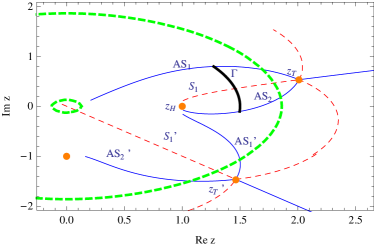
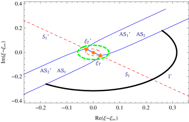
Figure 1: The Stokes diagram for $\omega=10(1-i)\pi T$ of the pure AdS black-hole background in the complex $z$ plane (left panel) and in the complex $\xi$ plane (right panel). We set $\pi T=1$. Anti-Stokes lines $AS_{1},AS_{2},AS_{3}$ are blue solid lines while Stokes lines $S_{1},S_{2},S_{3}$ are red dashed lines. The path $\Gamma$ connecting $AS_{1}$ and $AS_{2}$ is plotted as a thick black line. To determine the asymptotics (2), we connect the region $R_{2}$ (around $z=0$) and horizon $z_{H}$ via the path along $AS_{1},\Gamma$ and $AS_{2}$. We sketch the boundary of $R_{1}$ (where the WKB approximation applies) schematically using the green thick dashed lines. For completeness, we plot Stokes lines and anti-Stokes lines emanating from another turning point $z^{\prime}_{T}$ next to $z_{T}$.

We shall define point $\xi_{\infty}$ as the limit

$$\xi_{\infty}\equiv\mathop{\lim}\limits_{|\omega|\to\infty}\xi_{T}=\mathop{\lim}\limits_{|\omega|\to\infty}\int^{z_{T}}_{0}\frac{dz}{h(z)}$$ (37)

which exists if the integration in the above equation is convergent. To avoid ambiguity, we specify the path of the integration in Eq. (37) to be $AS_{1}$. Since, in the large $|\omega|$ limit, the region $R_{1}$ extends to the origin, the origin $z=0$ and the turning point $z_{T}$ are connected via $AS_{1}$ in that limit.

We now start using the WKB approximation to solve Eq. (26). Along $AS_{1}$, we can express $\Psi(\xi)$ using the standard WKB approximation:

$$\Psi_{B}(\xi)=\frac{B_{+}}{\sqrt{Q}}e^{i\int^{\xi}_{\xi_{\infty}}d\xi^{\prime}Q}+\frac{B_{-}}{\sqrt{Q}}e^{-i\int^{\xi}_{\xi_{\infty}}d\xi^{\prime}Q}\approx\frac{B_{+}}{\sqrt{Q}}e^{i\omega(\xi-\xi_{\infty})}+\frac{B_{-}}{\sqrt{Q}}e^{-i\omega(\xi-\xi_{\infty})}$$ (38)

as long as $\xi$ stays in region $R_{1}$. For convenience, we choose $\xi_{\infty}$ to be the lower limit of the “phase integration” in Eq. (38). A different choice of the lower limit of the integration would not affect our final results, but would complicate their derivation. Matching Eq. (38) with Eq. (34) in region $R_{2}$, we have:

$$\frac{A_{+}}{A_{-}}=\frac{B_{+}}{B_{-}}e^{-2i(\omega\xi_{\infty}-\delta_{0})}.$$ (39)

Similarly, along another anti-Stokes line $AS_{2}$ in region $R_{1}$, we could write $\Psi(\xi)$ as:

$$\Psi_{C}(\xi)\approx\frac{C_{+}}{\sqrt{Q}}e^{i\omega(\xi-\xi_{\infty})}+\frac{C_{-}}{\sqrt{Q}}e^{-i\omega(\xi-\xi_{\infty})}.$$ (40)

As both $\Psi_{B}(\xi)$ and $\Psi_{C}(\xi)$ represent the same solution of the Schrödinger equation (26) in different Stokes domains, $C_{\pm}$ can be expressed as a linear combination of $B_{\pm}$. To see that, we trace $\Psi_{B}(\xi)$ along a path $\Gamma$ connecting $AS_{1}$ and $AS_{2}$ while staying in $R_{1}$ as illustrated in Fig. 1. Along $\Gamma$, the “in-falling wave” term $e^{i\omega(\xi-\xi_{\infty})}$ is (exponentially) dominant over the second term $e^{-i\omega(\xi-\xi_{\infty})}$. Therefore $B_{+}$ must not change along $\Gamma$, no matter the value of $B_{-}$:

$$C_{+}=B_{+}.$$ (41)

On the other hand, if $B_{+}=0$, then $B_{-}$ cannot change along $\Gamma$, i.e., $C_{-}=B_{-}$ if $B_{+}=0$. As a result, we can express $C_{-}$ as:

$$C_{-}=B_{-}+SB_{+}$$ (42)

where the multiplier $S$ is the Stokes constant headingbook with respect to point $\xi_{\infty}$. The phenomenon that the coefficient of the subdominant solution is shifted by a product of $S$ and the coefficient of the (unchanged) dominant term is the well-known Stokes phenomenon.

In addition, near $z_{H}$, we have from Eq. (24): $\xi\approx-\log(z_{H}-z)/4$. Then selecting the solution $V_{-}(z)$ in Eq. (23) is equivalent to imposing the infalling wave condition:

$$C_{-}=0$$ (43)

along $AS_{2}$ Natario:2004jd . From Eq. (42), we obtain:

$$\frac{B_{+}}{B_{-}}=-\frac{1}{S}=e^{-\log S-i\pi}.$$ (44)

Substituting the above equation (44) in Eq. (39) and using the definition (31), we establish an asymptotic expression for $\mathcal{D}(\omega)$:

$$\omega\mathcal{D}(\omega)=\omega\xi_{\infty}-\frac{\pi}{4}(2\nu_{0}-1)-\frac{i}{2}\log S$$ (45)

and from Eq. (32) the asymptotic behavior of $\omega_{n}$ and $r_{n}$:

$$\omega_{n}=\left[n+\frac{i}{2\pi}\log S+\frac{1}{4}(2\nu_{0}-1)\right]{\omega_{0}},\qquad r_{n}=K\left({\omega_{0}}+\frac{i\omega^{2}_{0}}{2\pi S}\frac{\partial S}{\partial\omega}\Big{|}_{\omega=\omega_{n}}\right)$$ (46)

where

$$\omega_{0}=\pi/\xi_{\infty}.$$ (47)

3.4 The Stokes constant

To gain insight into how and whether $S$ should (or should not) depend on $\omega$, it is useful to think of the Stokes phenomenon in the following way meyer1989 . Both WKB solutions Eqs. (38) and (40), describe the same exact solution of the Schrödinger equation in two different Stokes sectors around the turning point. These approximate solutions are multivalued functions with a branching singularity at the turning point, $Q(\xi_{T})=0$. However, the exact solution of the Schrödinger equation is analytic at a regular point, such as the turning point. In order to match the absense of the branching singularity in the exact solution, the WKB solutions must compensate their discontinuity along a path winding around the turning point by a corresponding discontinuity in the coefficients $B$ and $C$. This is the essense of the Stokes phenomenon. For an isolated regular turning point this argument leads to the well-known value of $S=i$.

More importantly, this argument sheds light on the reason why the Stokes constant should have a different value in a special case when the turning point approaches a singularity of the Schrödinger potential in the limit $|\omega|\to\infty$, as it does in our case. Since, in this case, winding around the turning point, while staying in $R_{1}$, requires winding around the singularity also (as well as other turning points). If the singularity is a branching point of the exact solution, the discontinuity across the cut is reflected in the value of the Stokes constant, which thus depends on the nature of the singularity.

In fact, since we assume that, at large $z$, $U\sim z^{m}$ and $z/h$ vanishes to guarantee the convergence of the integration in Eq. (37), $\xi_{\infty}$ will always be a singular point of Eq. (26). If $\xi_{\infty}$ is a regular singular point of Eq. (26), $\Psi(\xi)$ can be expressed as a linear combination of two Frobenius series solutions: $(\xi-\xi_{\infty})^{f_{\pm}}(1+O(\xi-\xi_{\infty}))$ with $f_{\pm}$ being the indicial exponents and $f_{+}+f_{-}=1$. Taking the WKB solution around the point $\xi_{\infty}$ and matching the discontinuity of the exact solution, one finds the Stokes constant: $S=2i\cos[\pi(f_{+}-f_{-})/2]$ meyer1989 as we explain in detail in Appendix B. If the indicial exponents $f_{\pm}$ are independent of $\omega$, the resulting Stokes constant has no $\omega$ dependence either.

Even if $\xi_{\infty}$ is an irregular singular point of Eq. (26) one may still expect that determining $S$, though more involved, is still possible, perhaps along the lines of Ref. Meyer1983145 ; 10.1137/0514038 (see also Appendix B). From a more practical point of view, which we take in Sec. 4, even if one has not found an easy way to determine $S$ in that situation, one could attempt to fit asymptotic behavior of $\omega_{n}$ numerically using Eq. (49). If the quality of the fit is good and the resulting $\omega_{0}$ is close to the analytical expectation given by Eq. (37), then it is very likely that $S$ will approach a constant in large $|\omega|$ limit. In fact, that is what we observe for the soft-wall model at finite temperature (see Sec. (4) below).

In conclusion, we anticipate, on general grounds, that for a large class of theories the Stokes constant $S$ is a finite constant in the large $|\omega|$ limit. As a result, the asymptotics (2) are established.

Furthermore, to show that the summation over $(r_{n}-K\omega_{0})$ is convergent in the sum rule (4), we need to show that summation over $S^{-1}\partial S/\partial\omega$ terms is convergent. For sufficiently large $n$, we can replace the summation with integration. Then the existence of the large $|\omega|$ limit of $\log S$ would imply that the integration of $S^{-1}\partial S/\partial\omega$ is convergent and complete the derivation of the conductivity sum rule (4).

3.5 Examples and comparisons

The authors of Ref. Natario:2004jd have considered the cases that the Schrödinger Equation (26) takes the form:

$$\frac{d^{2}\Psi(\xi)}{d\xi^{2}}+\left[\omega^{2}-\frac{\nu^{2}_{\infty}-\frac{1}{4}}{(\xi-\xi_{\infty})^{2}}\right]\Psi(\xi)=0,\qquad\text{when}\qquad|z|\to\infty.$$ (48)

Then $f_{\pm}=\pm\nu_{\infty}-1/2$ and we have $S=2i\cos(\pi\nu_{\infty})$(see also Ref. headingbook ). Consequently, we read from Eq. (46) that:

$$\Delta=\left[\frac{i}{2\pi}\log(2i\cos(\pi\nu_{\infty}))+\frac{1}{4}(2\nu_{0}-1)\right]{\omega_{0}},$$ (49)

in complete agreement of the results of Ref. Natario:2004jd obtained by using the properties of the Bessel functions. For that reason, the first part of Eq. (46) is a generalization of the previous work. Although asymptotic behavior of $r_{n}$ can be calculated straightforwardly from the WKB approximations, the expression of $r_{n}$ in second part of Eq. (46), to the best of our knowledge, is new.

Finally, let us check the results obtained in this section in the case of pure thermal AdS black-hole background. In that case, $B(z)=-\log z$, $U(z)\approx-5z^{6}/4$ and $\xi\approx\xi_{\infty}+1/(3z^{3})$ when $|z|$ is large. In that limit, the Schrödinger equation (26) is reduced to Eq. (48) with $\nu_{\infty}=-1/3$. From Eq. (49) and recalling that $\nu_{0}=1$, we obtain $\Delta=0$ due to the cancellation between two terms in Eq. (49). Moreover, if $h(z)$ is a polynomial, as it is in the case at hand, $h(z)=1-z^{4}$, there is a simple way to evaluate $\xi_{\infty}$ in Eq. (37):

$$\xi_{\infty}=\frac{1}{2}\int^{z_{\infty}}_{-z_{\infty}}dz\frac{1}{h(z)}=\frac{1}{2}\oint_{\mathcal{C}}dz\frac{1}{h(z)}=-\pi i\sum_{z_{h}}\frac{1}{h^{\prime}(z_{h})}.$$ (50)

In the first equality we have used the property $h(z)=h(-z)$. The contour $\mathcal{C}$ is chosen to connect $\pm z_{\infty}$ by a straight line and a large semi-circle centered at the origin of the complex $z$ plane. As $|z_{\infty}|\to\infty$ when $|\omega|\to\infty$, the contribution from the integration along the semi-circle vanishes for $h(z)$ being a polynomial of $z^{2}$. Applying the Cauchy integral theorem to the integral, we obtain the rightmost expression in Eq. (50). The summation here denotes the summation over all $z_{h}$s, the zeros of $h(z)$, enclosed in the contour $\mathcal{C}$. In particular, for the pure AdS black-hole background, ${\rm Arg\,}z_{\infty}=\pi/12$ as can be seen in Fig. 1. Therefore $z=1,-i$ are the zeros of $h(z)$ enclosed in the contour $\mathcal{C}$. Consequently, $\xi_{\infty}=(1+i)/T$ thus $\omega_{0}=\pi/\xi_{\infty}=2(1-i)\pi T$ (we restored the units which were set by $\pi T=1$ in this Section). One can check that $\omega_{n},r_{n}$ given by Eq. (2) coincide with the quasi-normal spectrum of $\mathcal{N}=4$ SYM theory given by Eq. (17).

4 Examining the sum rule in the“soft-wall” model at finite temperature.

In this section, we will examine the sum rule (4) with the “soft-wall” model Karch:2006pv , a holographic QCD model, at finite temperature. With $\phi(z)=cz^{2}$ and $A(z)=-\log z$, the “soft-wall” model reproduces the Regge-like trajectory of the vector mesons, $m^{2}_{n}=4nc$, at zero temperature Karch:2006pv . Studying that model at finite temperature can provide a non-trivial check of the sum rule (4). It can also illustrate how the dissociation or “melting” of the bound-states is related to the increase in conductivity, the phenomenon which is relevant to the transport properties of sQGP.

Dimensionless ratios of physical quantities in the “soft-wall” model at finite temperature are fully controlled by the dimensionless parameter $\tilde{c}=c/(\pi T)^{2}$. To make the connection with the real world more tangible, we set the overall scale by taking $c=2.54$ GeV to fit the mass of the $J/\psi$ at zero temperature. Such a choice has been used in Ref. Fujita:2009ca ; Fujita:2009wc to study the thermal charmonium spectral functions.

Following Ref. Fujita:2009ca ; Fujita:2009wc ; Grigoryan:2010pj ; Herzog:2006ra ), we assume pure black-hole metric background, i.e, $h(z)=1-(z\pi T)^{4}$. We have calculated the first five quasi-normal modes $\omega_{n}$ and the corresponding rescaled residues $r_{n}$ numerically for temperature $T$ between $250$ MeV and $500$ MeV. For the soft-wall model at finite temperature, the point $\xi_{\infty}$ is an irregular singular point of Eq. (26). As we have explained in the previous section, we fit $\omega_{n}$ using Eq. (49) to obtain $\Delta$. Indeed, Eq. (49) provides a good fit for $\omega_{n}$s where $n=2,3,4,5$ and the resulting $\omega_{0}$ is close to the expected asymptotic value $2(1-i)\pi T$. To analyze separate contributions to the conductivity, we split the R.H.S of the sum rule (4) into two terms:

$$s_{1}=-{K}{\rm Im\,}(\omega_{0}),\qquad\text{and}\qquad s_{2}=-{2K}{\rm Im\,}\Delta+2\sum^{n_{\rm max}}_{n=1}{\rm Im\,}\left(r_{n}-K{\omega_{0}}\right).$$ (51)

where in practice we set $n_{\rm max}=5$. In Fig. 2, we plot $\sigma,s,s_{1},s_{2}$ and the total sum $s=s_{1}+s_{2}$ (normalized by $2\pi K$) versus $T$. We extract the conductivity via the analytic results of Ref. Iqbal:2008by (see also Ref. Grigoryan:2010pj ):

$$\sigma=2\pi KTe^{B(z_{H})}.$$ (52)

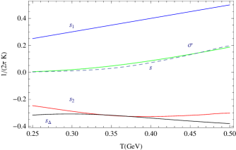
Figure 2: $\sigma$(Green), $s$(dashed), $s_{1}$(blue), and $s_{2}$(red) divided by the constant $2\pi K$ as a function of $T$. To evaluate $s_{2}$, we truncated the summation at $n=5$. We also plot the contribution from the $\Delta$ term to the total sum normalized by $2\pi K$: $s_{\Delta}=-2K{\rm Im\,}\Delta$ in black.

Obviously from the plot, the R.H.S of the sum rule (4) $s$ (dashed line), calculated numerically, is close to the conductivity $\sigma$(solid green line) given by Eq. (52) in the temperature range we are considering. We take that result as a numerical evidence that the sum rule (4) applies to the “soft-wall” model. Moreover, $s_{1}$ is linear in $T$ and has no $c$ dependence. Thus, we could interpret $s_{1}$ as the contribution to the conductivity from the thermal AdS background with no account of confinement effect introduced by parameter $c$. We also observe that $s_{2}$ is always negative. That can be thought of as a reflection of the physical fact that the presence of bound states reduces the number of the charge carriers in medium and lowers the conductivity. That effect is quantified by $s_{2}$. Finally, we note from Fig. 2 that $s_{2}$ in Eq. (51) is dominated by $s_{\Delta}=-2K{\rm Im\,}\Delta$ term in the range of the temperature we are studying. That would mean that in some cases, one may be able to use $-K{\rm Im\,}(\omega_{0}+2\Delta)$ as a reasonable estimate of $\sigma$.

5 Summary and discussion

We have shown that the current-current correlator in a theory with holographic dual description can be represented as a convergent infinite sum over the quasinormal mode poles Eq. (1). We have established the convergence by deriving the asymtpotic behavior of the quasinormal mode frequencies and residues Eq. (46) using the WKB, or phase integral, approach.

We have also established a sum rule relating conductivity $\sigma$ to the convergent infinite sum over quasinormal modes Eq. (4). We have checked this sum rule in the exactly solvable case of the ${\cal N}=4$ SUSY Yang-Mills theory. We studied the non-trivial example of the soft-wall holographic model numerically and found that the sum rule is in good agreement with analytically known value of the conductivity, and that the sum over the quasinormal modes is quickly saturated by a few lowest terms.

5.1 Spectral function

Using representation Eq. (1) for $G_{R}$ we can also obtain a corresponding convergent representation for the spectral function:

$$\rho(\omega)=\sigma\omega-\omega^{2}\sum_{n}{\rm Im\,}\left[\frac{r_{n}}{\omega-\omega_{n}}+\frac{\tilde{r}_{n}}{\omega-\tilde{\omega}_{n}}\right].$$ (53)

We have expressed the “gap” $\omega_{0}$ and “offset” $\Delta$ parameters of the quasinormal modes in terms of the singular point of the Schrödinger quation $\xi_{\infty}$ and the corresponding Stokes constant $S$, Eq. (46), (47). Further insight into the significance of $\xi_{\infty}$ (or $\omega_{0}$) and $S$ (or $\Delta$) may be obtained if one assumes that asymptotic expression of $\mathcal{D}(\omega)$ in Eq. (45) can be continued to the real axis ${\rm Arg}(\omega)=0$. Let us further assume that $U(z)$ and $h(z)$ are even functions of $z$. Then $\xi(z)$ defined by Eq. (24) is an odd function of $z$. Consequently, $U(\xi)$ is an even function of $\xi$. One can then argue that the corrections to Eq. (30) should be in even powers of $\omega^{-1}$. However, as $\rho(\omega)$ is an odd function of $\omega$, those power corrections may not affect the asymptotic behavior of $\rho(\omega)$. We could then use Eq. (30) and Eq. (45) to study the asymptotics of the spectral density:

$$\rho(\omega)\to\pi K\omega^{2}\left[1+2{\rm Im\,}(Se^{2i\omega\xi_{\infty}})\right]=\pi K\omega^{2}\left[1+2e^{-2\omega\xi_{I}}{\rm Im\,}(Se^{2i\omega\xi_{R}})\right]$$ (54)

where $\xi_{\infty}=\xi_{R}+i\xi_{I}$. The first term in the square brackets, $1$, on R.H.S of Eq. (54) is expected as $\rho(\omega)$ will asymptotically approach zero temperature limit. The next term explains the observation made on the basis of the numerical studies of Ref. Teaney:2006nc that “finite temperature result oscillates around the zero temperature result with exponentially decreasing amplitude.” The author of Ref. Teaney:2006nc argues that such behavior is intimately connected with the analytic structure stemming from the quasi-normal modes. Indeed, since ${\rm Im\,}\omega_{0}<0$ and thus $\xi_{I}>0$, Eq. (54) shows that $2\xi_{R}$ and $2\xi_{I}$ correspond to the oscillation frequency and the damping rate respectively. Our analysis suggests that such phenomenon is quite generic for theories with a gravity dual.

One can easily check the correctness of Eq. (54) with Eq. (16) for the $\mathcal{N}=4$ SYM in the strong coupling limit where the Green’s function is known analytically Myers2007 . In addition, one can extend our analysis to other channels, e.g., the shear channel, as well. For example, for $\mathcal{N}=4$ SYM in the strong coupling limit, again, $\xi_{\infty}=(1+i)/4T$, we then predict the damping rate of the corresponding spectral density to be $1/(2T)$ while by fitting numerics, the authors of Ref. Romatschke:2009ng obtained a damping rate of $.46/T$.

In passing, we also note that due to the asymptotic behavior in Eq. (54), the integral over $\omega^{2n-1}\delta\rho(\omega)$, where $\delta\rho(\omega)=\rho(\omega,T)-\rho(\omega,T=0)$, is convergent for any positive integer $n$. This suggests that for theories with a gravity dual, one could establish a family of f-sum rules forster1975hydrodynamic as discussed in Appendix C.

5.2 Conductivity

An insight into the meaning of the conductivity sum rule can be obtained by assuming a naive representation of the Green’s function $G_{R}(\omega)$ in terms of the quasinormal modes:

$$G_{R}(\omega)\stackrel{{\scriptstyle R}}{{=}}\sum_{n}\left[\frac{\omega_{n}^{2}r_{n}}{\omega-\omega_{n}}+\frac{\tilde{\omega}^{2}_{n}\tilde{r}_{n}}{\omega-\tilde{\omega}_{n}}\right]$$ (55)

This representation ignores the fact the the sum is divergent. In a certain sense, the convergent representation (1) is a regularized version of the naive representation (which is indicated by letter $R$ in (55)). Taking imaginary part in Eq. (55) and using Kubo formula (7) we would find

$$\sigma\stackrel{{\scriptstyle R}}{{=}}2{\rm Im\,}\sum_{n}r_{n}.$$ (56)

Again, this sum rule ignores divergence of the sum. We can think of Eq. (4) as the regularized form of this naive sum rule.

One could interpret the naive sum rule (56) as an expression of the following physical picture. Consider the behavior of quarkonia-like resonances as a function of temperature. As the temperature is increased the resonance poles in the Green’s function move into (the lower half of) the complex plane. The residues $r_{n}$, starting off as the real decay constants at $T=0$, acquire their imaginary parts at finite temperature and are thus related to the process of “melting” or dissociation of the resonances. As a bound state dissociates, the conductivity receives contribution from the freed charge carriers.

Although this picture is intuitive, its usefulness is limited, as the actual example we considered in Section  4 shows. We find that the dominant contribution to the conductivity comes from the first term $-K{\rm Im\,}(\omega_{0}+2\Delta)$ of the sum rule Eq. (4). This term could be thought of as the combined contribution of the whole tower of resonances as it is a result of the regularization of the divergent sum in Eq. (56).

Appendix A Redundant poles and $\omega=-2in\pi T$

We now discuss a subtle issue in the context of gauge/gravity dual on how to define $G_{R}(\omega)$ at following points:

$$\omega=-2ni\pi T,\qquad n=1,2,\ldots.$$ (57)

We consider the Frobenius power series expansion Eq. (58) near $z_{H}$:

$$V_{\pm}(z,\omega)=(z-z_{H})^{r_{\pm}}\sum^{\infty}_{j=0}c^{\pm}_{j}(\omega)(z-z_{H})^{j}$$ (58)

where the indicial exponents $r_{\pm}=\pm i\omega/4\pi T$ and coddingtonbook :

$$c^{-}_{j}(\omega)=\frac{F^{-}_{j}}{j(i\omega/(2\pi T)-j)}.$$ (59)

Here, $F^{-}_{j}$ is a linear combination of $c^{-}_{j-1},\ldots,c^{-}_{0}$ coddingtonbook :

$$F^{-}_{j}=\sum^{j-1}_{k=0}[(k+r_{-})\alpha_{j-k}+\omega^{2}\beta_{j-k}]c^{-}_{k}$$ (60)

and $\alpha_{j},\beta_{j}$ have no $\omega$ dependence coddingtonbook :

$$(z-z_{H})(B^{\prime}+\frac{h^{\prime}}{h})=\sum^{\infty}_{k=0}\alpha_{k}(z-z_{H})^{k},\qquad\frac{(z-z_{H})^{2}}{h^{2}}=\sum^{\infty}_{k=0}\beta_{k}(z-z_{H})^{k}.$$ (61)

As a result of Eq. (59,60,61), the coefficient $c^{-}_{j}(\omega)$ will be a meromorphic function of $\omega$ with simple poles at $\omega$ given by Eq. (57) for $j\geq n$. However, those singularities can be cured naturally by suitably choosing the overall constant $c^{-}_{0}$. For example, one may define:

$$c^{-}_{0}=\frac{1}{\Gamma(1-i\omega/(2\pi T))},$$ (62)

then the Frobenius solutions (58) are regular in the entire complex $\omega$ plane. Consequently, those points listed by Eq. (57) will not, in general, lead to any additional singularities of $G_{R}(\omega)$. Noting from Eq. (23) that $G_{R}(\omega)$ has no dependence on the overall normalization of the solution $V_{-}(\omega,z)$, a different choice of $c^{-}_{0}$ will not affect resulting $G_{R}(\omega)$.

In fact, those special points have been known as “redundant zeros (poles)” PhysRev.69.668 since long time ago in the context of the non-relativistic scattering. It has been shown Proc.Roy.Soc ; J.Math.Physic.1 that for the Schrödinger potential with the exponential tail:

$$U(\xi)\sim e^{-y\xi}\qquad\xi\to\infty$$ (63)

the infalling wave solutions $\Psi(\xi,\omega)$ will have simple poles at $\omega=-iny/2$. One can check from Eq. (27) and Eq. (24) that in our case, $y=4\pi T$, thus again we have Eq. (57). Historically, those poles are called “redundant poles” because they do not represent the true resonant states. In the context of the holographic correspondence, the name “redundant poles” may still be appropriate as they are not related to the singular points of the retarded Greens function $G_{R}(\omega)$. As a result, the singularities of $G_{R}(\omega)$ are only due to simple poles at $\omega_{n}(\tilde{\omega}_{n})$.

Appendix B The Stokes constant for a regular singular point

In this section, we will derive the Stokes constant with respect to a regular singular point of a Schrödinger-type equation

$$\frac{d^{2}\Psi}{dy^{2}}+\left(\lambda^{2}-U_{0}(y)\right)\Psi(y)=0.$$ (64)

Without losing generality, we set $y=0$ to be that regular singular point such that:

$$\mathop{\lim}\limits_{y\to 0}y^{2}U_{0}(y)=l^{2}$$ (65)

and $\lambda$ to be a real positive large parameter. Eq. (64) has two Frobenius series solutions:

$$\psi_{1}(y)=y^{f_{+}}g_{1}(y)$$ (66a)

$$\psi_{2}(y)=y^{f_{-}}g_{2}(y)$$ (66b)

where $g_{1}(y),g_{2}(y)$ are power series of $y$. The indicial exponents are the roots of the equation:

$$f^{2}-f-l^{2}=0.$$ (67)

One may note from Weda’s theorem that

$$f_{+}+f_{-}=1.$$ (68)

A solution of Eq. (64), $\Psi(y)$, can be expressed as a linear combination of $\Psi_{1}(y),\Psi_{2}(y)$, i.e.,

$$\Psi(y)=c_{1}\Psi_{1}(y)+c_{2}\Psi_{2}(y).$$ (69)

From Eq. (66), we also have:

$$\Psi(ye^{2\pi i})=c_{1}e^{2\pi if_{+}}\Psi_{1}(y)+c_{2}e^{2\pi if_{-}}\Psi_{2}(y);$$ (70a)

$$\Psi(ye^{-2\pi i})=c_{1}e^{-2\pi if_{+}}\Psi_{1}(y)+c_{2}e^{-2\pi if_{-}}\Psi_{2}(y).$$ (70b)

Multiplying Eq. (70a) and Eq. (70b) by $e^{-\pi i(f_{+}+f_{-})}$ and $e^{\pi i(f_{+}+f_{-})}$ respectively, then adding the results together, we have a connecting relation olver1974asymptotics :

$$2\cos[\pi(f_{+}-f_{-})]\Psi(y)=e^{-\pi i(f_{+}+f_{-})}\Psi(ye^{2\pi i})+e^{\pi i(f_{+}+f_{-})}\Psi(ye^{-2\pi i})=-[\Psi(ye^{2\pi i})+\Psi(ye^{-2\pi i})].$$ (71)

If we solve the Schrödinger equation (64) using WKB approximation, we find two turning points at $y=\pm l/\lambda$. For $\lambda\to\infty$ these points approach the singularity at $y=0$. In the region of $y$ not very close to the origin, where $\lambda^{2}\gg|U(y)|$, the solution $\Psi(y)$ can be approximated by a linear combination of two WKB solutions: $e^{\pm i\lambda y}$.

We plot the Stokes diagram schematically in Fig. 3. For large $\lambda$ the region where the WKB approximation breaks down shrinks to the origin. This region includes both turning points and the singularity at $y=0$. Since we are working outside that region, so that $\lambda^{2}\gg|U(y)|$, we can represent this non-WKB region by a single point at $y=0$. Only four anti-Stokes lines emanate from this region as shown in Fig. 3: two from each turning point, following the real axis in positive and negative directions.

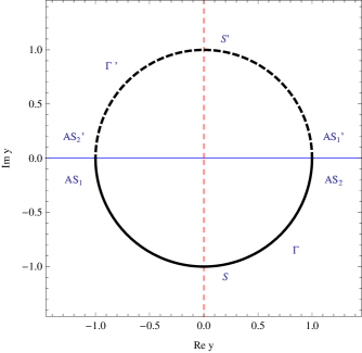
Figure 3: The schematic plot of the Stokes diagram for Eq. (64). One can compare it with Fig. 1. In large $|\omega|$, two turning points $\xi_{T},\xi_{T}^{\prime}$ are shrunk to $\xi_{\infty}$. What is more, the distance between $AS_{1}$ and $AS^{\prime}_{2}$(or $AS_{2}$ and $AS^{\prime}_{1}$) also vanishes. Therefore, schematically, we only draw two anti-Stokes lines in blue and two Stokes lines in red dashed line in this figure. We also plot the path $\Gamma$ in black thick line and $\Gamma^{\prime}$ black thick dashed line.

To determine the Stokes constant, we will consider a WKB solution defined by its value along the real axis:

$$\Psi_{0}(y)=e^{i\lambda y},\qquad\text{when Arg$\,y=0$}.$$ (72)

When continued counterclockwise from the positive real axis to the negative axis along $\Gamma^{\prime}$, $\Psi_{0}$ is unchanged as $e^{i\lambda y}$ is subdominant compared to $e^{-i\lambda y}$ in the upper half plane. If we go on continuing $\Psi_{0}(y)$ along $\Gamma$ from the negative real axis to the positive real axis, we will have:

$$\Psi_{0}(ye^{2\pi i})=e^{i\lambda y}+Se^{-i\lambda y}.$$ (73)

due to the Stokes phenomenon. Similar, when $\Psi_{0}(y)$ is continued clockwise from the positive real axis to the negative real axis along $\Gamma$, we have:

$$\Psi_{0}(ye^{-\pi i})=e^{i\lambda y}-Se^{-i\lambda y}.$$ (74)

Furthermore, when $\Psi_{0}(ye^{-\pi i})$ is continued clockwise from the negative real axis to the positive real axis along $\Gamma^{\prime}$, we obtain:

$$\Psi_{0}(ye^{-2\pi i})=(1+S^{2})e^{i\lambda y}-Se^{-i\lambda y}.$$ (75)

Substituting Eq. (73) and Eq. (75) in Eq. (71) and comparing the coefficient of $e^{\pm i\lambda y}$, we have:

$$S=\pm 2i\cos\left[\frac{\pi(f_{+}-f_{-})}{2}\right],$$ (76)

the desired Stokes constant.

As pointed out in Ref. olver1974asymptotics , if $y$ is an irregular singular point, in general, it is still true that there exist solutions with the properties:

$$\psi_{1}(ye^{2i\pi})=e^{2\pi if_{+}}\psi_{1}(y)$$ (77a)

$$\psi_{2}(ye^{2i\pi})=e^{2\pi if_{-}}\psi_{2}(y)$$ (77b)

with $f_{\pm}$ called “circuit exponents” olver1974asymptotics of the singularity, in analogy with indicial exponents. One then observes immediately the connecting relation (71) is also true for $y$ being an irregular singular point. Because of that, one may generalize the present approach to determine $S$ to the cases that $y$ is irregular as well.

Appendix C f-sum rules from holography

We now derive a family of f-sum rules  forster1975hydrodynamic for theories with a gravity dual. Due to the representation (1), we have the following dispersion relation:

$$\delta G_{R}(i\omega_{E})=\mathcal{P}(\omega)+\int^{\infty}_{-\infty}\frac{d\omega}{2\pi}\frac{\delta\rho(\omega)}{\omega-i\omega_{E}}$$ (78)

where $\mathcal{P}(\omega)$ is a polynomial of $\omega$. We denote by “$\delta$” the difference between the value of a function at temperature $T$ and the value of that function at zero temperature. For example, $\delta G_{R}(\omega,T)=G_{R}(\omega,T)-G_{R}(\omega,T=0)$. Applying the Borel transformation to Eq. (78), we have:

$$\hat{\mathcal{B}}_{1/t_{B}}\delta G_{R}(\omega_{E})=-2t_{B}\int^{\infty}_{0}\frac{d\omega}{2\pi}\delta\rho(\omega)\sin(\omega t_{B})$$ (79)

where we have used the fact that $\rho(\omega)$ is an odd function of $\omega$. We then consider the asymptotic expansion of $\delta G_{R}(i\omega_{E})$

$$\delta G_{R}(i\omega_{E})=\sum^{\infty}_{n=0}\frac{\delta h_{n}}{\omega_{E}^{2n}},\qquad\text{when}\qquad\omega_{E}\to\infty$$ (80)

where the coefficients $\delta h_{n}$ may be calculated from OPE. Applying the Borel transformation to Eq. (80), we have:

$$\hat{\mathcal{B}}_{1/t_{B}}\delta G_{R}(\omega_{E})=\sum^{\infty}_{n=0}\frac{\delta h_{n}}{(2n-1)!}t_{B}^{2n}.$$ (81)

Therefore $\delta h_{n}$ can be extracted by comparing the Taylor expansion coefficients of Eq. (81) with that of Eq. (79):

$$\delta h_{n}=\mathop{\lim}\limits_{t_{B}\to 0}\frac{d^{2n-1}}{dt_{B}^{2n-1}}\left[\int^{\infty}_{0^{+}}\frac{d\omega}{2\pi}\delta\rho(\omega)\sin(\omega t_{B})\right]=2(-1)^{n}\int^{\infty}_{0}\frac{d\omega}{2\pi}\omega^{2n-1}\delta\rho(\omega).$$ (82)

As the integral is convergent, we have interchanged the sequence of taking the limit and the integration. In literature, Eq. (82) is related to the f-sum rule. From the definition of $\rho(t)=\langle[J^{i}(t),J^{i}(0)]\rangle$ and Heinseberg’s equation of motion, we have:

$$\frac{d^{2n-1}}{dt^{2n-1}}\rho(t)=(-i)^{2n-1}\langle\underbrace{[\dots[}_{2n}J^{i}(t),J^{i}(0)],\underbrace{T^{00}(t)],\dots,T^{00}(t)]}_{2n-1}\rangle.$$ (83)

By the Fourier transformation and taking $t\to 0$ limit, we have:

$$\int^{\infty}_{-\infty}\frac{d\omega}{2\pi}\omega^{2n-1}\rho(\omega)=\langle\underbrace{[\dots[}_{2n}J^{i}(0),J^{i}(0)],\underbrace{T^{00}(0)],\dots,T^{00}(0)]}_{2n-1}\rangle.$$ (84)

Comparing sum rules (84,82), we have established an expression of $\delta h_{n}$:

$$\delta h_{n+1}=(-1)^{n}\delta\langle\underbrace{[\dots[}_{2n}J^{i}(0),J^{i}(0)],\underbrace{T^{00}(0)],\dots,T^{00}(0)]}_{2n-1}\rangle_{T}.$$ (85)

Finally, we list all the formulas of the Borel transformation that we have used

$$\hat{\mathcal{B}}_{1/t_{B}}\left(\frac{1}{\omega+s}\right)=t_{B}e^{-st_{B}},\qquad\hat{\mathcal{B}}_{1/t_{B}}\left(\frac{1}{\omega^{n}}\right)=\frac{1}{(n-1)!}t^{n}_{B},\qquad\hat{\mathcal{B}}_{1/t_{B}}\left(\log\omega\right)=-1$$ (86)

for reference. We have also used the property that $\hat{\mathcal{B}}$ gives zero when acting on polynomials of $\omega$.

References

- (1) PHENIX Collaboration, K. Adcox et. al., Formation of dense partonic matter in relativistic nucleus-nucleus collisions at rhic: Experimental evaluation by the phenix collaboration, Nucl.Phys. A757 (2005) 184–283, [nucl-ex/0410003].
- (2) B. Back, M. Baker, M. Ballintijn, D. Barton, B. Becker, et. al., The phobos perspective on discoveries at rhic, Nucl.Phys. A757 (2005) 28–101, [nucl-ex/0410022]. PHOBOS White Paper on discoveries at RHIC.
- (3) BRAHMS Collaboration, I. Arsene et. al., Quark gluon plasma and color glass condensate at rhic? the perspective from the brahms experiment, Nucl.Phys. A757 (2005) 1–27, [nucl-ex/0410020].
- (4) STAR Collaboration, J. Adams et. al., Experimental and theoretical challenges in the search for the quark gluon plasma: The star collaboration’s critical assessment of the evidence from rhic collisions, Nucl.Phys. A757 (2005) 102–183, [nucl-ex/0501009].
- (5) P. Petreczky and D. Teaney, Heavy quark diffusion from the lattice, Phys.Rev. D73 (2006) 014508, [hep-ph/0507318].
- (6) G. Aarts, C. Allton, J. Foley, S. Hands, and S. Kim, Spectral functions at small energies and the electrical conductivity in hot, quenched lattice qcd, Phys. Rev. Lett. 99 (2007) 022002, [hep-lat/0703008].
- (7) J. M. Maldacena, The large n limit of superconformal field theories and supergravity, Adv. Theor. Math. Phys. 2 (1998) 231–252, [hep-th/9711200].
- (8) S. S. Gubser, I. R. Klebanov, and A. M. Polyakov, Gauge theory correlators from non-critical string theory, Phys. Lett. B428 (1998) 105–114, [hep-th/9802109].
- (9) E. Witten, Anti-de sitter space and holography, Adv. Theor. Math. Phys. 2 (1998) 253–291, [hep-th/9802150].
- (10) D. R. Gulotta, C. P. Herzog, and M. Kaminski, Sum rules from an extra dimension, JHEP 01 (2011) 148, [arXiv:1010.4806].
- (11) E. Berti, V. Cardoso, and A. O. Starinets, Quasinormal modes of black holes and black branes, Class.Quant.Grav. 26 (2009) 163001, [arXiv:0905.2975].
- (12) G. T. Horowitz and V. E. Hubeny, Quasinormal modes of ads black holes and the approach to thermal equilibrium, Phys.Rev. D62 (2000) 024027, [hep-th/9909056].
- (13) A. Nunez and A. O. Starinets, Ads/cft correspondence, quasinormal modes, and thermal correlators in n = 4 sym, Phys. Rev. D67 (2003) 124013, [hep-th/0302026].
- (14) P. K. Kovtun and A. O. Starinets, Quasinormal modes and holography, Phys.Rev. D72 (2005) 086009, [hep-th/0506184].
- (15) A. O. Starinets, Quasinormal modes of near extremal black branes, Phys.Rev. D66 (2002) 124013, [hep-th/0207133].
- (16) D. Birmingham, I. Sachs, and S. N. Solodukhin, Conformal field theory interpretation of black hole quasi- normal modes, Phys. Rev. Lett. 88 (2002) 151301, [hep-th/0112055].
- (17) R. Baier, P. Romatschke, D. T. Son, A. O. Starinets, and M. A. Stephanov, Relativistic viscous hydrodynamics, conformal invariance, and holography, JHEP 04 (2008) 100, [arXiv:0712.2451].
- (18) J. Hong and D. Teaney, Spectral densities for hot qcd plasmas in a leading log approximation, Phys. Rev. C82 (2010) 044908, [arXiv:1003.0699].
- (19) D. Teaney, Finite temperature spectral densities of momentum and r- charge correlators in n = 4 yang mills theory, Phys. Rev. D74 (2006) 045025, [hep-ph/0602044].
- (20) I. Amado, C. Hoyos-Badajoz, K. Landsteiner, and S. Montero, Residues of correlators in the strongly coupled n=4 plasma, Phys.Rev. D77 (2008) 065004, [arXiv:0710.4458].
- (21) J. Natario and R. Schiappa, On the classification of asymptotic quasinormal frequencies for d-dimensional black holes and quantum gravity, Adv.Theor.Math.Phys. 8 (2004) 1001–1131, [hep-th/0411267].
- (22) A. Karch, E. Katz, D. T. Son, and M. A. Stephanov, Linear confinement and ads/qcd, Phys. Rev. D74 (2006) 015005, [hep-ph/0602229].
- (23) M. A. Shifman, A. Vainshtein, and V. I. Zakharov, Qcd and resonance physics. sum rules, Nucl.Phys. B147 (1979) 385–447.
- (24) R. C. Myers, A. O. Starinets, and R. M. Thomson, Holographic spectral functions and diffusion constants for fundamental matter, JHEP 0711 (2007) 091, [arXiv:0706.0162].
- (25) D. T. Son and A. O. Starinets, Minkowski space correlators in ads / cft correspondence: Recipe and applications, JHEP 0209 (2002) 042, [hep-th/0205051].
- (26) C. P. Herzog and D. T. Son, Schwinger-keldysh propagators from ads/cft correspondence, JHEP 03 (2003) 046, [hep-th/0212072].
- (27) J.Heading, An Introduction to Phase-integral Methods. Methuen, London, 1962.
- (28) R. E. Meyer, A simple explanation of the stokes phenomenon, SIAM Review 31 (1989), no. 3 pp. 435–445.
- (29) R. Meyer and J. Painter, Irregular points of modulation, Advances in Applied Mathematics 4 (1983), no. 2 145 – 174.
- (30) R. E. Meyer and J. F. Painter, Connection for wave modulation, .
- (31) M. Fujita, T. Kikuchi, K. Fukushima, T. Misumi, and M. Murata, Melting spectral functions of the scalar and vector mesons in a holographic qcd model, Phys. Rev. D81 (2010) 065024, [arXiv:0911.2298].
- (32) M. Fujita, K. Fukushima, T. Misumi, and M. Murata, Finite-temperature spectral function of the vector mesons in an ads/qcd model, Phys.Rev. D80 (2009) 035001, [arXiv:0903.2316].
- (33) H. R. Grigoryan, P. M. Hohler, and M. A. Stephanov, Towards the gravity dual of quarkonium in the strongly coupled qcd plasma, Phys.Rev. D82 (2010) 026005, [arXiv:1003.1138].
- (34) C. P. Herzog, A holographic prediction of the deconfinement temperature, Phys. Rev. Lett. 98 (2007) 091601, [hep-th/0608151].
- (35) N. Iqbal and H. Liu, Universality of the hydrodynamic limit in ads/cft and the membrane paradigm, Phys.Rev. D79 (2009) 025023, [arXiv:0809.3808].
- (36) S. Caron-Huot, Asymptotics of thermal spectral functions, Phys. Rev. D79 (2009) 125009, [arXiv:0903.3958].
- (37) P. Romatschke and D. T. Son, Spectral sum rules for the quark-gluon plasma, Phys. Rev. D80 (2009) 065021, [arXiv:0903.3946].
- (38) D. Forster, Hydrodynamic fluctuations, broken symmetry, and correlation functions. WA Benjamin, Inc., Reading, MA, 1975.
- (39) E. A.Coddington, An Introduction to Ordinary Differential Equations. Prentice-Hall, 1961.
- (40) S. T. Ma, Redundant zeros in the discrete energy spectra in heisenberg’s theory of characteristic matrix, Phys. Rev. 69 (Jun, 1946) 668.
- (41) R.E.Peierls, Complex eigenvalues in scattering theory, Proc.Roy.Soc(London).A 253 (1959) 16.
- (42) R.G.Newton, Analytic properties of radial wave functions, J.Math.Phys 1 (1960) 319.
- (43) F. Olver, Asymptotics and special functions. Academic Press, 1974.