Fully synchronous solutions and the synchronization phase transition for the finite-$N$ Kuramoto model

Abstract

We present a detailed analysis of the stability of synchronized solutions to the Kuramoto system of oscillators. We derive an analytical expression counting the dimension of the unstable manifold associated to a given stationary solution. From this we are able to derive a number of consequences, including: analytic expressions for the first and last frequency vectors to synchronize, upper and lower bounds on the probability that a randomly chosen frequency vector will synchronize, and very sharp results on the large $N$ limit of this model. One of the surprises in this calculation is that for frequencies that are Gaussian distributed the correct scaling for full synchrony is not the one commonly studied in the literature—rather, there is a logarithmic correction to the scaling which is related to the extremal value statistics of the random frequency vector.

1 Introduction

1.1 History of Kuramoto model

The study of synchronization of coupled nonlinear oscillators has a history that spans several centuries, starting with Huygens’ observation of synchronizing pendulum clocks [12, 3]. There has been a great body of work throughout this history studying such synchronization phenomena; for reviews see [25, 21, 30]. There are a wide variety of such models derived from a diverse collection of mathematical and scientific questions, including pulse-coupled [13, 20] and conservative [7, 8] models. These models arise in a number of contexts, including numerous biological applications [14, 17], and exhibit a diversity of behaviors.

A fundamental model of synchronization, however, is the case where we consider independent oscillators connected through dissipative coupling, and the fundamental question is [25, 26]: how do independent oscillators with different frequencies adjust themselves to produce a collective mode?

The system of coupled ordinary differential equations

$$\frac{d\theta_{i}}{dt}=\gamma\sum_{j}\sin(\theta_{j}-\theta_{i})$$

was first proposed by Kuramoto [15, 16] as a model for the synchronization of oscillators; this model, and variants, are widely known as the Kuramoto model. Since this time, the Kuramoto model has been a fundamental model for many types of systems exhibiting synchronization [2, 6, 27, 11] and related phenomena such as flocking [9, 10]. For reviews, see [26, 1]. Most work in this area has analyzed the Kuramoto model in the continuum limit, where the number is oscillators $N$ is formally allowed to go to infinity and the summation is replaced by an appropriate integral. Such formal calculations provide a tremendous amount of physical insight into the problem; however, it has proven to be difficult to make these approaches rigorous.

An alternative approach, attributed by Strogatz [26] to a series of lectures by Kopell, is to analyze the finite-$N$ problem carefully and then take the $N\to\infty$ limit. There have been a few papers which have established rigorous results on the existence and stability of synchronized solutions [28, 29, 19, 18] but to date this the finite-$N$ problem has been only partially understood. In this paper we carry out a substantial portion of this program. We focus on the case of full synchrony, where all of the oscillators rotate with the same angular frequency. We derive new characterizations of the stable regions, which permit a detailed understanding of the region in frequency space where full synchronization occurs. In particular we are able to identify a large subset of the stable region, in the form of the Voronoi cell of a well-understood high dimensional lattice. Using this we find upper and lower bounds on the probability that the system undergoes full synchronization.

1.2 Problem Formulation

The standard formation of the Kuramoto problem is as follows: Consider a weighted (directed) graph $G=(V,E)$ and denote $\gamma_{ij}>0$ as the weight of edge $i\to j$. For any $\omega\in\mathbb{R}^{N}$, define the dynamical system on $\theta\in\mathbb{T}^{N}$ by

$$\frac{d}{dt}\theta_{i}=\omega_{i}+\sum_{j}\gamma_{ji}\sin(\theta_{j}-\theta_{i}).$$ (1.1)

One of the more common choices of interaction graph is the symmetric all-to-all graph where we assume that all the $\gamma_{ij}$ are equal. We thus consider the system

$$\frac{d}{dt}\theta_{i}=\omega_{i}+\gamma\sum_{j}\sin(\theta_{j}-\theta_{i}),$$ (1.2)

or, defining the function ${\mathbf{f}}\colon\mathbb{T}^{n}\to\mathbb{R}^{n}$ coordinatewise as

$$f_{i}({\boldsymbol{\theta}})=\sum_{j}\sin(\theta_{j}-\theta_{i}),$$ (1.3)

we can write (1.2) as

$$\frac{d}{dt}{\boldsymbol{\theta}}={\boldsymbol{\omega}}+\gamma{\mathbf{f}}({\boldsymbol{\theta}}).$$ (1.4)

Remark 1.1

Note that we have not rescaled the coupling coefficient in (1.2); the typical scaling chosen for Kuramoto is $\gamma/N$. We will refer to this scaling below as the “classical scaling”. One of the results of this paper is that the classical scaling is only the correct scaling for certain problems, and not for others. For the problem where the frequencies $\omega_{i}$ are chosen from a Gaussian distribution, for instance, we shall see that the correct scaling differs from the classical one by a logarithmic term.

Remark 1.2

It is worth noting that this flow is a gradient flow, if one considers the angles as lying in the covering space ${\mathbb{R}}^{N}$ rather than ${\mathbb{T}}^{N}$. The flow can be written as

$$\frac{d{\boldsymbol{\theta}}}{dt}=\nabla L$$

where the energy $L$ is given by

$$L=\langle{\boldsymbol{\omega}},{\boldsymbol{\theta}}\rangle+\gamma\sum_{i,j}\cos(\theta_{i}-\theta_{j})-N.$$

Here the constant $-N$ is chosen for convenience and obviously doesn’t influence the dynamics. It is common to work with the “order parameter” $R$

$$R^{2}({\boldsymbol{\theta}})=\left(\sum_{i}\cos(\theta_{i})\right)^{2}+\left(\sum_{i}\sin(\theta_{i})\right)^{2}=N+\sum_{i,j}\cos(\theta_{i}-\theta_{j}),$$

which gives the energy function as

$$L=\langle{\boldsymbol{\omega}},{\boldsymbol{\theta}}\rangle+R^{2}({\boldsymbol{\theta}}).$$

Thus the Kuramoto flow tries to maximize an energy given by a sum of two terms. The first term acts to align the flow with the frequency vector ${\boldsymbol{\omega}},$ while the second acts to increase the order parameter. All of the structure that arises in Kuramoto model is due to a competition between these two effects.

The fundamental question we consider is the question of whether (1.2) admits a fully synchronous solution, as we now define:

Definition 1.1

For a given value of the frequency vector ${\boldsymbol{\omega}}$ we say that the Kuramoto model exhibits full synchrony if (1.2) with $\gamma=1$ admits a stationary solution ${\boldsymbol{\theta}}$ which is asymptotically stable, i.e. we have a solution to the equation

$${\mathbf{f}}({\boldsymbol{\theta}})=-{\boldsymbol{\omega}}$$ (1.5)

such that, if we define the Jacobian matrix

$$J=\nabla_{\boldsymbol{\theta}}f,$$ (1.6)

then $J$ is negative semi-definite with a one-dimensional kernel. If such a solution exists, we call it a fully synchronous solution.

Remark 1.1

It is not hard to see that, for fully synchronous solutions, we will have

$$\max_{i,j}\sup_{t\in[0,\infty)}\left\|{\theta_{i}(t)-\theta_{j}(t)}\right\|<\infty.$$

However, note that due to the continuous symmetry of (1.2), these fully synchronous solutions can be moving in the same co-rotating frame. The Kuramoto model also permits partially synchronous solutions where a large mass of the oscillators are fixed relative to each other, and some subset precesses relative to them. We do not consider such solutions in this work, q.v. the discussion in Section 6 below.

The results of the paper are organized as follows. In Section 2 we give an almost complete characterization of the ${\boldsymbol{\omega}}$ which give rise to fully synchronous solutions; in particular, we show that this set is convex, identify many important points on the boundary of this set, and explicitly determine the convex hull of these points. We would like to characterize “how easy” it is for a Kuramoto problem to fully synchronize, but there are many senses in which one can pose this problem; we consider two different cases below.

For example, we could pose the following question: given ${\boldsymbol{\omega}}\in\mathbb{R}^{N}$, define $\gamma^{\star}({\boldsymbol{\omega}})$ as the minimal $\gamma$ for which (1.4) has a fully synchronous solution. Of course the presence of synchrony is invariant under a rescaling in time, so one may as well assume that $\left|{{\boldsymbol{\omega}}}\right|=1$. The motivates the definition

Definition 1.2

Define the lower and upper critical couplings ${\gamma}_{{{\mathsf{min}}}}(N)$ and ${\gamma}_{{{\mathsf{max}}}}(N)$ in the following way:

$${\gamma}_{{{\mathsf{min}}}}(N):=\inf_{\begin{subarray}{c}{\boldsymbol{\omega}}\in\mathbb{R}^{N}\\ \left|{{\boldsymbol{\omega}}}\right|=1\end{subarray}}\gamma^{\star}({\boldsymbol{\omega}}),\quad{\gamma}_{{{\mathsf{max}}}}(N):=\sup_{\begin{subarray}{c}{\boldsymbol{\omega}}\in\mathbb{R}^{N}\\ \left|{{\boldsymbol{\omega}}}\right|=1\end{subarray}}\gamma^{\star}({\boldsymbol{\omega}})$$ (1.7)

Roughly ${\gamma}_{{{\mathsf{min}}}}(N)$ characterizes the minimal coupling constant we should choose to get full synchrony, and the values of ${\boldsymbol{\omega}}$ for which the infimum is attained (by symmetry there are many) can be thought of as the “most easily synchronizable frequency(s)”; analogously ${\gamma}_{{{\mathsf{max}}}}(N)$ characterizes the most difficult frequencies. to synchronize, and gives the largest necessary coupling constant. For coupling constants above this value all frequency vectors synchronize. The quantities ${\gamma}_{{{\mathsf{min}}}}$ and ${\gamma}_{{{\mathsf{max}}}}$ are closely related to the quantity $K_{c}$ studied by Verwoerd and Mason in their work[28, 29]: ${\gamma}_{{{\mathsf{min}}}}(N)$ is essentially the minimum of $K_{c}$ over the unit circle, and ${\gamma}_{{{\mathsf{max}}}}$ the maximum.

We study ${\gamma}_{{{\mathsf{min}}}}(N),{\gamma}_{{{\mathsf{max}}}}(N)$ in Section 3, and give bounds which show the different asymptotic scalings of these quantities. We will show that in the limit $N\to\infty$, ${\gamma}_{{{\mathsf{min}}}}(N)\sim N^{-3/2}$ and ${\gamma}_{{{\mathsf{max}}}}(N)\sim N^{-1}$. In particular, synchrony “turns on” much earlier than the classical scaling, although it “fills up” in a way consistent with the classical scaling.

A different method of choosing ${\boldsymbol{\omega}}$, which is very common in the literature, is to assume that the entries of ${\boldsymbol{\omega}}$ are chosen independently from some probability distribution, i.e. that the $\omega_{n}$ are iid random variables. In Section 4 we consider this question; stated precisely, we proceed as follows. Fix $\gamma>0$ and $N$, and choose $\omega_{n}$ independently from a Gaussian distribution with mean zero and unit variance, i.e. the $\omega_{n}$ are independent $N(0,1)$. Define $\mathcal{P}_{{{\mathsf{sync}}}}(\gamma,N)$ as the probability of (1.2) having a fully synchronous solution. Define $\varphi(N):=\sqrt{2\ln(N)}/(N+1)$, and what we show below in Theorem 4.1 is

$$\lim_{N\to\infty}\mathcal{P}_{{{\mathsf{sync}}}}(\delta\varphi(N),N)=\begin{cases}0,&\delta<1,\\ 1,&\delta>2.\end{cases}$$ (1.8)

In particular, this implies that $\mathcal{P}_{{{\mathsf{sync}}}}(\gamma/N,N)\to 0$ for any $\gamma$, so that in the classical scaling the probability of full synchrony is zero. In fact, we will show in Proposition 4.5 that the probability of full synchrony decays to zero exponentially fast as $N\to\infty$. We show that this anomalous scaling is closely related to the extreme value statistics for a Gaussian distribution, and is to be expected for any distribution of frequencies which is not of compact support.

Finally, in Section 6 we finish with some comments about the different choices of scaling and why they arise and present a few open questions.

2 Characterization of the Stable Set

In this section we write down a relatively complete description of the set of ${\boldsymbol{\omega}}$ for which (1.2) admits a stable fully synchronous solution. We do this by proving an index theorem which counts the dimension of the unstable manifold to any stationary solution. The stable synchronous solutions are then those for which the unstable manifold is zero dimensional.

2.1 Notation

We consider the finite $N$ Kuramoto model with uniform sine coupling on the complete graph, which we repeat

$$\frac{d}{dt}{\boldsymbol{\theta}}={\boldsymbol{\omega}}+\gamma{\mathbf{f}}({\boldsymbol{\theta}})$$ (1.4)

Note that

$$\sum_{i=1}^{N}f_{i}({\boldsymbol{\theta}})=0$$

for all ${\boldsymbol{\theta}}$, due to a telescoping sum. Therefore we have

$$\frac{d}{dt}\sum\theta_{i}=\sum\omega_{i}=:\Omega.$$ (2.1)

This means that, if $\Omega\neq 0$, the center of mass of the system precesses around the circle with a constant velocity. Using the change of variables $\tilde{\theta}_{i}=\theta_{i}-N^{-1}\Omega t$ puts us into a corotating frame and allows us to assume without loss of generality that $\sum_{i}\omega_{i}=0$.

The function ${\mathbf{f}}\colon\mathbb{T}^{n}\to\mathbb{R}^{n}$ is a natural map from the configuration space ${\mathbb{T}}^{n}$ to the frequency space ${\mathbb{R}}^{n}$. Assuming some convexity conditions which will be established later, the frequency vector ${\boldsymbol{\omega}}$ is the convex dual variable to the angle vector ${\boldsymbol{\theta}}$. It will also be convenient to think of this as a map ${\mathbf{f}}\colon\mathbb{T}^{n-1}\to\mathbb{R}^{n-1}\cong\mathbb{R}^{n}/\{1,1,\dots,1\}$ — this can be done, for example, by fixing a single $\theta_{n}$.

The Jacobian of this mapping controls the stability of the synchronized state, and it is crucial to have a good understanding of set of parameter values for which the Jacobian is negative semi-definite. This motivates the following definition:

Definition 2.1

We define ${\mathcal{S}}_{\theta}$ to be the set of configurations for which the Jacobian $\frac{\partial{\mathbf{f}}}{\partial{\bf\theta}}$ is negative semi-definite with a one dimensional kernel. The boundary of this set is obviously the set of configurations for which the Jacobian $\frac{\partial{\mathbf{f}}}{\partial{\bf\theta}}$ is negative semi-definite with a kernel of dimension two or more.

Throughout the paper calligraphic capital letters will denote sets of particular interest, with a subscript of $\theta$ denoting sets in the configuration space $\mathbb{T}^{n-1}$ and a subscript $\omega$ denoting the corresponding sets in the frequency space. For instance if $\mathcal{S}_{\boldsymbol{\theta}}$ denotes the set of asymptotically stable stationary configurations then $\mathcal{S}_{\boldsymbol{\omega}}$, the set of frequencies admitting an asymptotically stable stationary configuration, is simply the image of $\mathcal{S}_{\boldsymbol{\theta}}$ under the map ${\mathbf{f}}$:

$${\mathbf{f}}:\mathcal{S}_{\boldsymbol{\theta}}\mapsto\mathcal{S}_{\boldsymbol{\omega}}$$

It is clear that $\mathcal{S}_{\boldsymbol{\omega}}$ is the important object for studying synchronization: all questions about the probability of (full) synchrony are questions about the size of $\mathcal{S}_{\boldsymbol{\omega}}$ in some measure. One of the key ingredients in this is a good characterization of $\mathcal{S}_{\boldsymbol{\omega}}$.

2.2 Index Theorem

In this section we prove an index theorem which counts the dimension of the unstable manifold to the synchronized state. The basic idea of this section is that the Jacobian takes a relatively simple form, as it can be written as a rank two perturbation of a diagonal matrix. An application of a rank-two perturbation formula gives a straightforward count of the number of positive eigenvalues.

Definition 2.2

Given a matrix $A$, we define the three quantities $n_{+}(A),n_{-}(A),n_{0}(A)$ as the number of eigenvalues of $A$ with positive, negative, and zero real parts, respectively. We will refer to these as the indices of $A$. (Given a vector field ${\mathbf{f}}$ with fixed point ${\boldsymbol{\theta}}^{*}$, we will abuse notation and refer to the indices of ${\boldsymbol{\theta}}^{*}$ when we mean the indices of the Jacobian of the vector field at ${\boldsymbol{\theta}}$.)

A straightforward calculation gives the following expression for the Jacobian matrix

$$J_{ij}({\boldsymbol{\theta}}):=\displaystyle\frac{\partial{f_{i}}}{\partial{\theta_{j}}}({\boldsymbol{\theta}})=\begin{cases}\cos(\theta_{i}-\theta_{j}),&i\neq j\\ -\sum_{k\neq i}\cos(\theta_{k}-\theta_{i}),&i=j.\end{cases}$$ (2.2)

Using the cosine angle addition formula, we have

$$J=-D+{\mathbf{v}}\otimes{\mathbf{v}}+{\mathbf{w}}\otimes{\mathbf{w}}$$ (2.3)

where the vectors ${\mathbf{v}}$ and ${\mathbf{w}}$ are defined by

$${\mathbf{v}}=\left(\begin{array}[]{c}\sin(\theta_{1})\\ \sin(\theta_{2})\\ \vdots\\ \sin(\theta_{n})\\ \end{array}\right),\qquad{\mathbf{w}}=\left(\begin{array}[]{c}\cos(\theta_{1})\\ \cos(\theta_{2})\\ \vdots\\ \cos(\theta_{n})\\ \end{array}\right),$$ (2.4)

$D$ is the diagonal matrix

$$D_{ij}=\delta_{ij}\sum_{k}\cos(\theta_{k}-\theta_{i}),$$ (2.5)

and $\otimes$ denotes the usual outer product $\left({\bf a}\otimes{\bf b}\right)_{ij}=a_{i}b_{j}.$

The Jacobian is a positive semi-definite rank two perturbation of a diagonal matrix, a fact which figured in the analysis of [19]. The spectrum of a low rank perturbation of an operator can be computed explicitly in terms of the spectrum of the unperturbed operator together with some information about the inverse of the (unperturbed) operator, a fact usually known as the Aronszajn-Krein formula [24]. Here the unpertubed operator is diagonal and can thus be trivially inverted, and one can get a reasonably complete description of the spectrum.

Thus we proceed as follows. Since the full Jacobian is a rank two perturbation of the diagonal, the indices of $J$ and $D$ can differ by at most two. We will first compute the index of $D$, then compute the difference of indices explicitly.

Definition 2.3

Given a configuration ${\boldsymbol{\theta}}$, we define the complex order parameter

$$Re^{i\psi}=\frac{1}{N}\sum_{n=1}^{N}e^{i\theta_{n}}.$$ (2.6)

Proposition 2.1

Using the $O(1)$ invariance, rotate the configuration so that the order parameter is on the positive real axis. Then we have

$$n_{+}(-D)=\#\left\{\theta_{i}|\cos(\theta_{i})<0\right\}$$

Proof. Since $D$ is diagonal we just have to count the number of negative entries on the diagonal. We have

$$D_{ii}=\sum_{k}\cos(\theta_{k}-\theta_{i})=\cos(\theta_{i})\sum_{k}\cos(\theta_{k})+\sin(\theta_{k})\sum\sin(\theta_{i})$$ (2.7)

which we recognize as the $(1,0)$ component of the order parameter rotated through angle $\theta_{i}$. The number of times this is negative is the number of angles in the range $(\pi/2,3\pi/2)$. $\blacksquare$

Remark 2.1

Proposition 2.1 is equivalent to the calculations done in Section 4 of [19].

Since the perturbation is rank two, and one of the eigenvalues of the Jacobian is zero, if $D$ is negative-definite then there is only one eigenvalue whose sign is to be determined.

Theorem 2.2

Suppose $D$ is invertible. Define the following quantity:

$$\tau=\sum_{i}\frac{1}{\sum_{j}\cos(\theta_{j}-\theta_{i})}=\left\langle{{{\mathbf{v}}}},{{D^{-1}{\mathbf{v}}}}\right\rangle+\left\langle{{{\mathbf{w}}}},{{D^{-1}{\mathbf{w}}}}\right\rangle=\left\langle{{\mathbf{1}}},{{D^{-1}\mathbf{1}}}\right\rangle.$$ (2.8)

Then we have

$$n_{+}(J)=n_{+}(-D)+\begin{cases}0,&\tau<2,\\ 1,&\tau>2.\end{cases}$$ (2.9)

Proof. We proceed by a homotopy argument in the spirit of the Birman–Schwinger Principle (see, for instance, the discussion on page 98 of Volume 4 of the text of Reed and Simon [22]). Consider the one parameter family of operators

$$J_{\eta}=-D+\eta({\mathbf{v}}\otimes{\mathbf{v}}+{\mathbf{w}}\otimes{\mathbf{w}})$$ (2.10)

Clearly $J_{0}=-D$ and $J_{1}=J$. Since ${\mathbf{v}}\otimes{\mathbf{v}}+{\mathbf{w}}\otimes{\mathbf{w}}$ is non-negative, all eigenvalues are non-decreasing functions of $\eta$. We can detect eigenvalues crossing from the left half-plane to the right half-plane by detecting changes in the dimension of the kernel of $J_{\eta}$. $J_{\eta}$ has non-trivial kernel if there is a vector ${\mathbf{{x}}}$ with $J_{\eta}{\mathbf{{x}}}=\mathbf{0}$, or

$$-D{\mathbf{{x}}}+\eta(\left\langle{{{\mathbf{v}}}},{{{\mathbf{{x}}}}}\right\rangle{\mathbf{v}}+\left\langle{{{\mathbf{w}}}},{{{\mathbf{{x}}}}}\right\rangle{\mathbf{w}})=0.$$

Solving for ${\mathbf{{x}}}$ gives

$${\mathbf{{x}}}=\eta(\left\langle{{{\mathbf{v}}}},{{{\mathbf{{x}}}}}\right\rangle D^{-1}{\mathbf{v}}+\left\langle{{{\mathbf{w}}}},{{{\mathbf{{x}}}}}\right\rangle D^{-1}{\mathbf{w}}).$$ (2.11)

Taking the inner product with ${\mathbf{v}}$ and ${\mathbf{w}}$ gives

$$\left\langle{{{\mathbf{v}}}},{{{\mathbf{{x}}}}}\right\rangle =\eta(\left\langle{{{\mathbf{v}}}},{{{\mathbf{{x}}}}}\right\rangle\left\langle{{{\mathbf{v}}}},{{D^{-1}{\mathbf{v}}}}\right\rangle+\left\langle{{{\mathbf{w}}}},{{{\mathbf{{x}}}}}\right\rangle\left\langle{{{\mathbf{v}}}},{{D^{-1}{\mathbf{w}}}}\right\rangle),$$ (2.12)

$$\left\langle{{{\mathbf{w}}}},{{{\mathbf{{x}}}}}\right\rangle =\eta(\left\langle{{{\mathbf{v}}}},{{{\mathbf{{x}}}}}\right\rangle\left\langle{{{\mathbf{w}}}},{{D^{-1}{\mathbf{v}}}}\right\rangle+\left\langle{{{\mathbf{w}}}},{{{\mathbf{{x}}}}}\right\rangle\left\langle{{{\mathbf{w}}}},{{D^{-1}{\mathbf{w}}}}\right\rangle).$$ (2.13)

This can be thought of as a linear system for the quantities

$$a_{1}=\left\langle{{{\mathbf{v}}}},{{{\mathbf{{x}}}}}\right\rangle,\quad a_{2}=\left\langle{{{\mathbf{w}}}},{{{\mathbf{{x}}}}}\right\rangle,$$ (2.14)

which can be written in matrix form as

$$M_{\eta}\left(\begin{array}[]{c}a_{1}\\ a_{2}\\ \end{array}\right):=\left(\begin{array}[]{cc}\eta\left\langle{{{\mathbf{v}}}},{{D^{-1}{\mathbf{v}}}}\right\rangle-1&\eta\left\langle{{{\mathbf{v}}}},{{D^{-1}{\mathbf{w}}}}\right\rangle\\ \eta\left\langle{{{\mathbf{w}}}},{{D^{-1}{\mathbf{v}}}}\right\rangle&\eta\left\langle{{{\mathbf{w}}}},{{D^{-1}{\mathbf{w}}}}\right\rangle-1\\ \end{array}\right)\left(\begin{array}[]{c}a_{1}\\ a_{2}\\ \end{array}\right)=\left(\begin{array}[]{c}0\\ 0\\ \end{array}\right).$$ (2.15)

There exists a nontrivial solution to (2.15) (i.e., $M_{\eta}$ has a nontrivial kernel) if and only if $J_{\eta}$ itself has a nontrivial kernel. Thus we want to count zeroes of $\det(M_{\eta})$ for $\eta\in(0,1)$. Initially $M_{0}=-{\bf I}_{2\times 2}$ has two negative eigenvalues. At $\eta=1$ we have that $M_{1}$ is singular so that one of the eigenvalues is zero. $M$ is a linear matrix value function of $\eta$, and the linear term

$$\left(\begin{array}[]{cc}\left\langle{{{\mathbf{v}}}},{{D^{-1}{\mathbf{v}}}}\right\rangle&\left\langle{{{\mathbf{v}}}},{{D^{-1}{\mathbf{w}}}}\right\rangle\\ \left\langle{{{\mathbf{w}}}},{{D^{-1}{\mathbf{v}}}}\right\rangle&\left\langle{{{\mathbf{w}}}},{{D^{-1}{\mathbf{w}}}}\right\rangle\\ \end{array}\right)$$

is positive definite, so the eigenvalues of $M$ are increasing functions of $\eta$. This implies that all eigenvalue crossings are transverse left to right and so the number of positive eigenvalues of the full matrix is determined by the non-zero eigenvalue of $M_{1}.$ If this is negative there have been no eigenvalue crossings, and if this is positive there has been one. Since one eigenvalue is zero the other is equal to the trace, which is

$$\mathop{\rm Tr}\nolimits(M_{1})=-1+\left\langle{{{\mathbf{v}}}},{{D^{-1}{\mathbf{v}}}}\right\rangle-1+\left\langle{{{\mathbf{w}}}},{{D^{-1}{\mathbf{w}}}}\right\rangle=\left\langle{{\mathbf{1}}},{{D^{-1}\mathbf{1}}}\right\rangle-2=\tau-2.$$

Thus if this quantity is positive a single eigenvalue has crossed into the right half-plane and $n_{+}(-D)=n_{+}(J)+1$. If this quantity is negative then no eigenvalues have crossed and the count is the same, $n_{+}(-D)=n_{+}(J)$.

$\blacksquare$

Remark 2.1

Since the Jacobian matrix for the Kuramoto model is of the form of a graph Laplacian, the Kirchoff matrix tree theorem can be applied. This expresses the product of the non-zero eigenvalues in terms of a sum over spanning trees of a product over edges in the spanning tree of the edge weights. In our case the edge weights may not be positive, but the standard proofs of the matrix tree theorem still hold in this case. Our formula above suggests that the product over the non-zero eigenvalues of the Jacobian should be proportional to the quantity

$$\mathop{\rm Tr}\nolimits(M_{1})=\tau-2.$$

One can check that this is the case, and actually compute the constant of proportionality. This gives the following unusual combinatorial identity

$$\sum_{{\mathcal{T}}\in{\mathcal{S}}}\prod_{e\in{\mathcal{T}}}\cos(\theta_{e})=\frac{2\prod_{i}\sum_{j}\cos(\theta_{i}-\theta_{j})-\sum_{k}\prod_{i\neq k}\sum_{j}\cos(\theta_{i}-\theta_{j})}{\sum_{i,j}\cos(\theta_{i}-\theta_{j})}.$$ (2.16)

Here ${\mathcal{S}}$ is the set of all spanning trees on $N$ points (of which there are $N^{N-2}$), ${\mathcal{T}}$ is an element of ${\mathcal{S}}$, a spanning tree, $e$ is an edge in the spanning tree, and if the edge $e$ connects vertices $l$ and $m$ then $\theta_{e}=\theta_{l}-\theta_{m}.$ The left-hand side of (2.16) comes from the matrix tree theorem, and the righthand side comes from directly evaluating the product of the non-zero eigenvalues using arguments similar to those given above. This identity is not used in the current paper — we really only need the formula derived in Theorem 2.2 — but the existence of such a formula is extremely interesting. It suggests that there may be much more algebraic structure in this problem than is readily apparent.

Having a concise index count for the Jacobian makes it possible to begin to make an analytical description of this region. Our first observation is:

Lemma 2.3

Let $\mathcal{S}_{\boldsymbol{\theta}}$ denote the region in configuration space where the there exists a stable synchronized solution. This region is simply connected and is given by the connected component of $\tau^{-1}([1,2))$ that contains the origin.

Proof. To see that the stability region is simply connected, and that it is the component containing the origin, we give an explicit stability-preserving retraction of any stable steady state onto the stable steady state ${\boldsymbol{\theta}}=\mathbf{0}$. Consider, for example, the retraction ${\boldsymbol{\theta}}(\zeta)=\zeta{\boldsymbol{\theta}}$. When $\zeta=1$, we have the original steady state ${\boldsymbol{\theta}}$, and when $\zeta=0$, we have the stable steady state $\theta_{i}=0$.

The derivative of the Jacobian with respect to the homotopy parameter is given by

$$\left(\frac{\partial J}{\partial\zeta}\right)_{ij}=\left\{\begin{array}[]{c}(\theta_{j}-\theta_{i})\sin(\zeta(\theta_{j}-\theta_{i}))\qquad i\neq j\\ -\sum_{k}(\theta_{k}-\theta_{i})\sin(\zeta(\theta_{k}-\theta_{i})).\qquad i=j\end{array}\right.$$

A necessary condition for stability is that $|\theta_{i}-\theta_{j}|\leq\pi$ for all $i,j.$ This implies that $(\theta_{j}-\theta_{i})\sin(\zeta(\theta_{j}-\theta_{i}))$ is a positive quantity thus that $\frac{\partial J}{\partial\zeta}$ is positive definite. Thus as the homotopy parameter $\zeta$ is decreased from $1$ to $0$ the eigenvalues of the Jacobian decrease, and all stable stationary states are contractible onto the state ${\bf\theta}=0$ in a way that increases stability. This establishes the simple connectedness of $\mathcal{S}_{\boldsymbol{\theta}}$ and thus, by continuity, $\mathcal{S}_{\boldsymbol{\omega}}$.

$\blacksquare$

We need something stronger than Lemma 2.3. In order to derive lower bounds on quantities related to the probability of stabilization we would like a much stronger result: namely that the stable region is a convex set. This is the content of the next few results.

Definition 2.4

Define $\kappa_{i}({\boldsymbol{\theta}})=\sum_{j}\cos(\theta_{j}-\theta_{i})$. Define $\mathcal{S}_{\boldsymbol{\theta}}$ as the subset of $\mathbb{T}^{n}$ for which we have $\kappa_{i}\geq 0$ and $\tau=\sum_{i=1}^{n}\kappa_{i}^{-1}\leq 2$, and $\mathcal{S}_{\boldsymbol{\omega}}$ as the image of $\mathcal{S}_{\boldsymbol{\theta}}$ under the map ${\bf f}.$

Remark 2.2

Note that by Proposition 2.1 and Theorem 2.2, $\mathcal{S}_{\boldsymbol{\omega}}$ is precisely the set of ${\boldsymbol{\omega}}$ such that ${\boldsymbol{\omega}}={\mathbf{f}}({\boldsymbol{\theta}})$ for some ${\boldsymbol{\theta}}$, and the Jacobian (2.3) is negative semi-definite; in short, those ${\boldsymbol{\omega}}$ for which we have fully synchronous solutions.

The above characterization of the stable region is difficult to use in practice, since one needs to find the image under a reasonably complicated map of a region defined by a transcendental equation. The following lemma shows that the boundary of this region is actually a connected piece of an algebraic variety.

Lemma 2.4

The stable frequency set $\mathcal{S}_{\boldsymbol{\omega}}$ can be defined algebraically as follows: It is the solution set of

$$\kappa_{i}^{2}+\omega_{i}^{2} =\sum_{j}\kappa_{j}$$ (2.17)

$$\kappa_{i} >0$$ (2.18)

$$\sum\frac{1}{\kappa_{i}} <2$$ (2.19)

$$\sum\omega_{i} =0$$ (2.20)

Since all $\kappa_{i}>0$, (2.19) implies $\kappa_{i}>\frac{1}{2}$ for all $i$. Also note that summing the first equation over $i$ shows

$${\boldsymbol{\kappa}}^{2}+{\boldsymbol{\omega}}^{2}=N\langle{\bf 1},{\boldsymbol{\kappa}}\rangle$$

or, equivalently

$$|{\boldsymbol{\kappa}}-N{\bf 1}|^{2}+{\boldsymbol{\omega}}^{2}=\frac{N^{3}}{4}$$

and thus the entire stable region lies in a sphere of radius ${\boldsymbol{\omega}}\leq\frac{N^{\frac{3}{2}}}{2}$.

Proof. The main observation is the following: squaring $\kappa_{i}$ and $\omega_{i}$ and adding them gives

$$\kappa_{i}^{2}+\omega_{i}^{2} =\sum_{j,j^{\prime}}\cos(\theta_{j}-\theta_{i})\cos(\theta_{j^{\prime}}-\theta_{i})+\sin(\theta_{j}-\theta_{i})\sin(\theta_{j^{\prime}}-\theta_{i})$$

$$=\sum_{j,j^{\prime}}\cos(\theta_{j}-\theta_{j^{\prime}}),$$

or

$${\bf F}_{i}(\kappa,\omega):=\kappa_{i}^{2}+\omega_{i}^{2}-\sum_{j=1}^{n}\kappa_{j}=0,\mbox{ for all }i.$$ (2.21)

Computing the Jacobian of the function ${\bf F}$ we find that

$$\frac{\partial{\bf F}}{\partial{\bf\kappa}}=\left(\begin{array}[]{ccccc}2\kappa_{1}-1&-1&-1&\ldots&-1\\ -1&2\kappa_{2}-1&-1&\ldots&-1\\ \vdots&\vdots&\ddots&\ddots&-1\\ -1&-1&-1&\ldots&2\kappa_{n}-1\end{array}\right)$$ (2.22)

It is straightforward to check that the determinant of this Jacobian is

$$\det(\frac{\partial{\bf F}}{\partial{\bf\kappa}})=2^{n-1}\prod_{i=1}^{N}\kappa_{i}\left(2-\sum\frac{1}{\kappa_{i}}\right)$$

All of the principal minors are of the same form, so it is easy to check that this matrix is positive definite in the stable region $\sum\frac{1}{\kappa_{i}}<2$, so an implicit function argument shows that we can define ${\bf\kappa}$ as a function of $\bf\omega.$ The second equation is equivalent to the condition $n_{-}(D)=0$, while the third condition is equivalent to to the condition that $n_{-}(D)=n_{-}(-J)$. Finally the last equation restricts to the subspace $\langle{\bf\omega},{\bf 1}\rangle=0$. $\blacksquare$

Given this algebraic representation of the stable set it is relatively straightforward to check that the region is convex.

Theorem 2.5

The set $\mathcal{S}_{\boldsymbol{\omega}}$ is convex.

Proof. We will first show that the Hessian of $\kappa_{i}$ (with respect to ${\boldsymbol{\omega}}$!) is negative definite for each $i$. This implies that $\frac{1}{\kappa_{i}}$ is a convex function. This implies that $\tau,$ being a sum of convex functions, is convex. Finally, the region $\mathcal{S}_{\boldsymbol{\omega}}=\{{\boldsymbol{\omega}}\mid\tau({\boldsymbol{\omega}})\leq 2\}$, is bounded by a level set of a convex function and is therefore a convex set.

Differentiating (2.21) twice gives

$$2\kappa_{i}\displaystyle\frac{\partial^{2}{\kappa_{i}}}{\partial{\omega_{k}}\partial{\omega_{l}}}+2\displaystyle\frac{\partial{\kappa_{i}}}{\partial{\omega_{k}}}\displaystyle\frac{\partial{\kappa_{i}}}{\partial{\omega_{l}}}+2\delta_{k,i}\delta_{k,l}=\sum_{j=1}^{N}\displaystyle\frac{\partial^{2}{\kappa_{j}}}{\partial{\omega_{k}}\partial{\omega_{l}}}$$ (2.23)

Recalling the definition of $\mathbf{M}$ in (2.22), (2.23) can be written as a matrix equation in the form

$$\mathbf{M}(\kappa)h_{kl}=2\displaystyle\frac{\partial{\kappa_{i}}}{\partial{\omega_{k}}}\displaystyle\frac{\partial{\kappa_{i}}}{\partial{\omega_{l}}}+2\delta_{k,i}\delta_{k,l},$$ (2.24)

where we have the unknown $N$-vector

$$h_{kl}:=\left\{\displaystyle\frac{\partial^{2}{\kappa_{i}}}{\partial{\omega_{k}}\partial{\omega_{l}}}\right\}_{i=1}^{N}.$$

To clear up a potential confusion: here we think of (2.23) as an equation where we fix $k,l$ which determines a vector where we vary the functions $\kappa_{i}$ in the entries of the vector.

If $\mathbf{M}(\kappa)$ is invertible, then

$$h_{kl}=\mathbf{M}^{-1}\left(2\displaystyle\frac{\partial{\kappa_{i}}}{\partial{\omega_{k}}}\displaystyle\frac{\partial{\kappa_{i}}}{\partial{\omega_{l}}}+2\delta_{k,i}\delta_{k,l}\right).$$ (2.25)

We have already shown that $\mathbf{M}$ is invertible in the proof of Lemma 2.4 above, and now we compute the inverse exactly. Write $\mathbf{M}=\mathbf{D}+\mathbf{1}\otimes\mathbf{1}^{t}$, where $\mathbf{D}$ is the diagonal matrix whose $i$th entry is $-2\kappa_{i}$. Using the Aronszajn-Krein formula , or checking directly, we have that

$$\mathbf{M}^{-1}=\mathbf{D}^{-1}-\frac{(\mathbf{D}^{-1}\mathbf{1})\otimes(\mathbf{D}^{-1}\mathbf{1})^{t}}{1+\left\langle{{\mathbf{1}}},{{\mathbf{D}^{-1}\mathbf{1}}}\right\rangle}.$$ (2.26)

In this case, we have

$$\left((\mathbf{D}^{-1}\mathbf{1})\otimes(\mathbf{D}^{-1}\mathbf{1})^{t}\right)_{ij}=\frac{1}{4\kappa_{i}\kappa_{j}},\quad 1+\left\langle{{\mathbf{1}}},{{\mathbf{D}^{-1}\mathbf{1}}}\right\rangle=1+\sum_{i=1}^{n}\frac{1}{2\kappa_{i}},$$ (2.27)

so that

$$\left(\mathbf{M}^{-1}\right)_{ij}=-\frac{\delta_{ij}}{2\kappa_{i}}-\frac{1}{1+\sum_{i=1}^{n}\frac{1}{2\kappa_{i}}}\frac{1}{4\kappa_{i}\kappa_{j}}.$$

In particular, every element of $\mathbf{M}^{-1}$ is negative for $\kappa\in\mathcal{S}_{\boldsymbol{\omega}}$ by (2.19). Then we can write

$$\frac{\partial^{2}{\kappa_{i}}}{\partial{\omega_{k}}\partial{\omega_{l}}}=2\delta_{kl}(\mathbf{M}^{-1})_{ik}+\sum_{j=1}^{N}(\mathbf{M}^{-1})_{ij}\left(2\displaystyle\frac{\partial{\kappa_{i}}}{\partial{\omega_{k}}}\displaystyle\frac{\partial{\kappa_{i}}}{\partial{\omega_{l}}}\right).$$ (2.28)

This is a negative definite matrix: it is given by linear combination of $N+1$ matrices with negative coefficients, and each of these matrices are manifestly positive definite — the first is diagonal with positive entries, and the rest are of the form $(\nabla\kappa_{j})\otimes(\nabla\kappa_{j})$.

Finally, we note that if $\kappa_{i}$ has a negative definite Hessian, then $\kappa_{i}^{-1}$ has a positive definite Hessian. To see this, write $\nu_{i}=1/\kappa_{i}$, and we have

$$\frac{\partial^{2}{\nu_{i}}}{\partial{\theta_{\alpha}}\partial{\theta_{\beta}}}({\boldsymbol{\theta}})=\frac{-\kappa_{i}({\boldsymbol{\theta}})\displaystyle\frac{\partial^{2}{\kappa_{i}}}{\partial{\theta_{\alpha}}\partial{\theta_{b}}}({\boldsymbol{\theta}})+2\displaystyle\frac{\partial{\kappa_{i}}}{\partial{\theta_{\alpha}}}({\boldsymbol{\theta}})\displaystyle\frac{\partial{\kappa_{i}}}{\partial{\theta_{\beta}}}({\boldsymbol{\theta}})}{\kappa_{i}({\boldsymbol{\theta}})^{3}}.$$ (2.29)

Since $\kappa_{i}>0$, this implies that the Hessian of $\nu_{i}$ is positive definite. Since $\tau=\sum\kappa_{i}^{-1}$ is convex the stable set $\mathcal{S}_{\boldsymbol{\theta}}$, which is bounded by a level set of $\tau$, is convex. $\blacksquare$

2.3 Lower Bounds on the stable set

We next characterize a subregion of $\mathcal{S}_{\boldsymbol{\theta}}$ for which we are guaranteed stability. The first region takes the form of a curvilinear polytope, and is the image of a cube under the map $\bf f$. We will show that the vertices of this polytope actually lie on the boundary of $\mathcal{S}_{\boldsymbol{\theta}}$ as well. This region is more difficult to deal with analytically, so we introduce a second (flat) polytope which is determined by the convex hull of the vertices of the curvilinear polytope. This polytope is the Voronoi cell of the root lattice $A_{n}$ and as such its properties are well-studied . This allows us to get very good estimates geometric quantities such as the volume, the probability that a random vector lies in the stable synchronous region, etc.

Definition 2.5

We define the stable cube $\mathcal{C}$ to be

$${\mathcal{C}}:=\left\{{\boldsymbol{\theta}}\mid{\boldsymbol{\theta}}\in[0,\pi/2]^{N}\right\}.$$ (2.30)

and the set $\mathcal{V}$ to be the vertex set of the the cube with two vertices removed:

$$\mathcal{V}:=\{{\boldsymbol{\theta}}|\forall i,\theta_{i}\in\{0,\pi/2\}\}/\{(0,0,0,\ldots,0),(\frac{\pi}{2},\frac{\pi}{2},\frac{\pi}{2},\ldots,\frac{\pi}{2})\}.$$ (2.31)

Remark 2.3

One can consider vertices of the $n$-cube as representing the partition of the $n$ oscillators into two sets. In this interpretation $\mathcal{V}$ represents the partition of the $n$ oscillators into two non-empty sets. We will see below that the set $\mathcal{V}$ represents points in ${\mathbb{T}}^{N}$ that map to points on the boundary of $\mathcal{S}_{\boldsymbol{\omega}}$. The points $(0,0,0,\ldots,0)$ and $(\frac{\pi}{2},\frac{\pi}{2},\frac{\pi}{2},\ldots,\frac{\pi}{2})$ map to the interior of $\mathcal{S}_{\boldsymbol{\omega}}$ (in fact to the origin - the most stable configuration).

Lemma 2.6

The Jacobian is positive semi-definite on the cube $\mathcal{C}$. Moreover,

$$\dim(\ker(J))=\begin{cases}1,&{\boldsymbol{\theta}}\in{\mathcal{C}}/{\mathcal{V}},\\ 2,&{\boldsymbol{\theta}}\in{\mathcal{V}}.\end{cases}$$ (2.32)

Proof. If $\theta_{i}\in(0,\pi/2)$, then $\theta_{i}-\theta_{j}\in(-\pi/2,\pi/2)$ for all $i,j$ and thus $\cos(\theta_{i}-\theta_{j})>0$ for all $i,j$. Then the Jacobian matrix (1.6) takes the form of a weighted graph Laplacian on the complete graph with positive weights. (Said another way, $J$ has zero row sums and positive off-diagonal entries.) The dimension of the kernel of a graph Laplacian is equal to the number of connected components of the graph . Since none of the weights vanish, the dimension of the kernel is equal to $1$.

When ${\boldsymbol{\theta}}$ is on the boundary of $\mathcal{C}$, some of the weights may vanish, if the corresponding angles differ by exactly $\pi/2$. At the level of the graph, this amounts to decomposing the vertex set of the graph into two sets (one corresponding to $\theta_{i}=0$ and the other to $\theta_{i}=\frac{\pi}{2}$) and breaking all connections between the two sets. For the complete graph on $N$ nodes, this will disconnect the graph only if all points belong to one of these sets and neither one is empty. These configurations correspond exactly to points in $\mathcal{V}$. $\blacksquare$

We have defined a cube in configuration space where the stationary solutions are at least marginally stable, and the vertices of this region actually lie on the stability boundary. Next we characterize the shape of the corresponding region in frequency space.

Proposition 2.7

The image of $\mathcal{V}$ under the map ${\mathbf{f}}$ gives $2^{N}-2$ distinct frequency vectors. These vectors form (up to scaling) the vertices of $V(A_{n})$, the Voronoi cell of the root lattice $A_{N}$. Equivalently $V(A_{N})$ is the projection of the cube $[-\frac{\gamma N}{2},\frac{\gamma N}{2}]^{N}$ onto the $(N-1)$-dimensional plane normal to $\mathbf{1}$ in $R^{N}$.

Proof. It is easy to check directly that the image of $\mathcal{V}$ under the map ${\bf f}$ consists of vectors of the following form: if the vertex has $i$ angles of $0$ and $j$ angles of $\frac{\pi}{2}$ then the image is a permutation of the vector

$${\bf\omega}=\gamma(\underbrace{i,i,i,\ldots,i}_{j~{}~{}{\rm times}},\underbrace{-j,-j,-j,\ldots,-j}_{i~{}~{}{\rm times}})$$

where $i+j=N$. It is a reasonably well-known fact (see, for instance, Conway and Sloane [5] Chapter 21.3B) that the Voronoi cell around the origin of the root lattice $A_{N}$ has vertices given by vectors of the form

$${\bf v}=(\underbrace{\frac{i}{N},\frac{i}{N},\frac{i}{N},\ldots,\frac{i}{N}}_{j~{}~{}{\rm times}},\underbrace{-\frac{j}{N},-\frac{j}{N},-\frac{j}{N},\ldots,-\frac{j}{N}}_{i~{}~{}{\rm times}})$$

and is the projection of the unit cube $[-\frac{1}{2},\frac{1}{2}]^{N}$ onto the $(N-1)$-plane of mean zero vectors.

$\blacksquare$

Remark 2.4

The root lattice $A_{N}$ and the associated polytope arise in a surprising number of areas of mathematics including Lie algebras and root systems, Coxeter groups, coding theory, etc. The appearance here is perhaps not so surprising since the symmetry group of the Kuramoto problem, $S_{N}\times S_{2}$ (corresponding to permutation of the oscillators and ${\bf\theta}\mapsto-{\bf\theta}$), is the same as the symmetry group of the $A_{N}$ lattice.

Corollary 2.8

$\mathrm{cl}(\mathcal{S}_{\boldsymbol{\omega}})$ contains $V(A_{n})$ and the image of the vertex set ${\mathbf{f}}(\mathcal{V})$ lies on the boundary of $\mathcal{S}_{\boldsymbol{\omega}}$.

Proof. This is clear from the proposition above: a convex polytope is equal to the convex hull of its vertices, and the convexity of $\mathcal{S}_{\boldsymbol{\omega}}$ implies that the convex hull of a collection of boundary points is contained in the closure. $\blacksquare$

It is worth noting that there is a relatively easily computable set of points lying on the boundary on the stability region. While we have not had occasion to use this fact in the present paper this fact may prove useful for improving the current bounds, and is presented here.

Proposition 2.9

The stable region contains the (suitably scaled) dual polytope to the Voronoi cell $V(A_{N})$. The vertices of this dual polytope are given by the vectors

$$\pm\omega_{N}(1,0,0,\ldots,-1)$$

and all permutations, where $\omega_{N}$ is the number

$$\omega_{N}:=\frac{1}{16\sqrt{2}}\left(\sqrt{32+(N-1)^{2}}+3(N-1)\right)\sqrt{16+(N-1)\sqrt{32+(N-1)^{2}}-(N-1)^{2}}$$

Proof. The configurations which correspond to these frequencies are those with a group of $N-2$ angles at the origin and two others offset symmetrically from these:

$$\theta_{i}=\begin{cases}-x,&i=0,\\ 0,&i\in(2,N-1),\\ x,&i=N\end{cases}$$

The corresponding frequency vector is

$$\omega_{i}=((N-1)\sin(x)+\sin(2x),0,0,\ldots,0,-(N-1)\sin(x)-\sin(2x)).$$

If one maximizes the length of this frequency vector over all $x$ then one finds the expression above.

$\blacksquare$

3 Upper and Lower Bounds on $\gamma$

We first consider a formal argument as to the sizes of the vertex set in frequency space, i.e. the set ${\mathbf{f}}(\mathcal{V})$.

Definition 3.1

We define the frequency vectors ${{\boldsymbol{\omega}}}_{{{\mathsf{min}}}},{{\boldsymbol{\omega}}}_{{{\mathsf{max}}}}$ as follows:

$${{\boldsymbol{\omega}}}_{{{\mathsf{min}}}}:=\pm(1,1,\dots,1,-(N-1))^{t}$$ (3.1)

for all $N$. We define ${{\boldsymbol{\omega}}}_{{{\mathsf{max}}}}$ differently if $N$ is even or odd. If $N$ is even, we define ${{\boldsymbol{\omega}}}_{{{\mathsf{max}}}}$ as that vector whose first $N/2$ components are $N/2$, and whose last $N/2$ components are $-N/2$. If $N$ is odd, we define ${{\boldsymbol{\omega}}}_{{{\mathsf{max}}}}$ to be the vector with the first $(N-1)/2$ entries are $(N+1)/2$, and whose remaining entries are $-(N-1)/2$. In summary,

$${{\boldsymbol{\omega}}}_{{{\mathsf{max}}}}:=\begin{cases}(\underbrace{N/2,N/2,\dots,N/2}_{N/2},\underbrace{-N/2,-N/2,\dots,-N/2}_{N/2}),&N\mbox{ even,}\\ \underbrace{(N+1)/2,\dots,(N+1)/2}_{(N-1)/2},\underbrace{-(N-1)/2,\dots,-(N-1)/2}_{(N+1)/2},&N\mbox{ odd.}\end{cases}$$ (3.2)

Lemma 3.1

We have

$$\min_{{\boldsymbol{\theta}}\in\mathcal{V}}\left\|{{\mathbf{f}}({\boldsymbol{\theta}})}\right\|^{2}=N(N-1),\quad\max_{{\boldsymbol{\theta}}\in\mathcal{V}}\left\|{{\mathbf{f}}({\boldsymbol{\theta}})}\right\|^{2}=\begin{cases}N^{3}/4,&N\mbox{ even,}\\ N(N^{2}-1)/4,&N\mbox{ odd.}\end{cases}$$ (3.3)

Moreover, the ${\boldsymbol{\omega}}$ which minimize (resp. maximize) in (3.3) are permutations of ${{\boldsymbol{\omega}}}_{{{\mathsf{min}}}}$ (resp. ${{\boldsymbol{\omega}}}_{{{\mathsf{max}}}}$).

Proof. First note that $\left|{\mathcal{V}}\right|=2^{N}-2$ since we choose all vertices of the cube except two. Given ${\boldsymbol{\theta}}\in\mathcal{V}$, let $i\in 1,\dots,N-1$ be the number of entries of ${\boldsymbol{\theta}}$ which are equal to $0$ and $j=N-i$ be the number which are equal to ${\pi}/{2}$. Everything is the same up to permutation, so replace ${\boldsymbol{\theta}}$ with the vector

$${\boldsymbol{\theta}}^{*}=(\underbrace{0,0,\dots,0}_{i},\underbrace{\pi/2,\pi/2,\dots,\pi/2}_{j})^{t}.$$

Then

$${\boldsymbol{\omega}}^{*}={\mathbf{f}}({\boldsymbol{\theta}}^{*})=(\underbrace{j,j,\dots,j}_{i},\underbrace{-i,-i,\dots,-i}_{j})^{t}$$ (3.4)

We have

$$\left\|{{\boldsymbol{\omega}}^{*}}\right\|^{2}=i^{2}j+ij^{2}=ijN.$$

Clearly, to minimize this, we choose $i=N-1$ and $j=1$ (or vice-versa), and this gives ${\boldsymbol{\omega}}^{*}={{\boldsymbol{\omega}}}_{{{\mathsf{min}}}}$, and $\left\|{{{\boldsymbol{\omega}}}_{{{\mathsf{min}}}}}\right\|^{2}=N(N-1)$.

To maximize this, it depends on the parity of $N$; if $N$ is even, we choose $i=j=N/2$, and if $N$ is odd, we choose $i=\lfloor{N/2}\rfloor=(N-1)/2$. In either case we obtain ${{\boldsymbol{\omega}}}_{{{\mathsf{max}}}}$ as defined above. We calculate that for $N$ even, $\left\|{{{\boldsymbol{\omega}}}_{{{\mathsf{max}}}}}\right\|^{2}=N^{3}/4$, and for $N$ odd, $\left\|{{{\boldsymbol{\omega}}}_{{{\mathsf{max}}}}}\right\|^{2}=N(N^{2}-1)/4$.

$\blacksquare$

Remark 3.1

Notice that, for all $N$, $\left\|{{{\boldsymbol{\omega}}}_{{{\mathsf{max}}}}}\right\|^{2}=N^{3}/4+o(N^{3})$. The ${\boldsymbol{\theta}}$’s corresponding to ${{\boldsymbol{\omega}}}_{{{\mathsf{min}}}},{{\boldsymbol{\omega}}}_{{{\mathsf{max}}}}$ have a relatively simple characterization. The minimum vertex can be described as “a herd of sheep and a lone wolf”: $(N-1)$ oscillators at $\theta_{i}=0$ and $1$ oscillator at $\theta_{i}=\frac{\pi}{2}.$ The maximum vertex can be described as the state of “two competing cliques”. Finally, note that in any case, the vertices are really only distinguished by the size of the partitions $i$ and $j$, and thus there are $\lfloor\frac{N+1}{2}\rfloor$ different types of vertex.

Lemma 3.2

We have

$${\gamma}_{{{\mathsf{min}}}}(N)=\frac{1}{\sup_{{\boldsymbol{\theta}}\in\mathcal{S}_{\boldsymbol{\theta}}}\left\|{{\mathbf{f}}({\boldsymbol{\theta}})}\right\|},\quad{\gamma}_{{{\mathsf{max}}}}(N)=\frac{1}{\inf_{{\boldsymbol{\theta}}\in\mathcal{S}_{\boldsymbol{\theta}}}\left\|{{\mathbf{f}}({\boldsymbol{\theta}})}\right\|},\quad$$ (3.5)

Proof. Recall the definition of ${\gamma}_{{{\mathsf{min}}}}(N),{\gamma}_{{{\mathsf{max}}}}(N)$:

$${\gamma}_{{{\mathsf{min}}}}(N):=\inf_{\begin{subarray}{c}{\boldsymbol{\omega}}\in\mathbb{R}^{N}\\ \left|{{\boldsymbol{\omega}}}\right|=1\end{subarray}}\gamma^{\star}({\boldsymbol{\omega}}),\quad{\gamma}_{{{\mathsf{max}}}}(N):=\sup_{\begin{subarray}{c}{\boldsymbol{\omega}}\in\mathbb{R}^{N}\\ \left|{{\boldsymbol{\omega}}}\right|=1\end{subarray}}\gamma^{\star}({\boldsymbol{\omega}})$$ (1.7)

Moreover, notice that multiplying the right-hand side of 1.2 by a scalar does not change anything about the existence or stability of a fixed point. Choose $\left\|{{\boldsymbol{\omega}}}\right\|=1$, and if we try to solve

$$\gamma{\mathbf{f}}({\boldsymbol{\theta}})=-{\boldsymbol{\omega}},$$

we have to have $\gamma\left\|{{\mathbf{f}}({\boldsymbol{\theta}})}\right\|=1$, or

$$\gamma\geq\frac{1}{\sup_{{\boldsymbol{\theta}}\in\mathcal{S}_{\boldsymbol{\theta}}}\left\|{{\mathbf{f}}({\boldsymbol{\theta}})}\right\|}.$$

Since $\mathcal{S}_{\boldsymbol{\theta}}$ is open, this bound is saturated and gives us ${\gamma}_{{{\mathsf{min}}}}(N)$. The opposite argument works for ${\gamma}_{{{\mathsf{max}}}}(N)$. $\blacksquare$

Theorem 3.3

Recall the definition of ${\gamma}_{{{\mathsf{min}}}},{\gamma}_{{{\mathsf{max}}}}$ in (1.7) above. Then

$${\gamma}_{{{\mathsf{min}}}}(N)=\begin{cases}2N^{-3/2},&N\mbox{ even,}\\ 2N^{-3/2}+O(N^{-5/2}),&N\mbox{ odd,}\end{cases}$$ (3.6)

and

$$\frac{1}{\sqrt{N(N-1)}}\leq{\gamma}_{{{\mathsf{max}}}}(N)\leq\frac{\sqrt{2}}{\sqrt{N(N-1)}}$$ (3.7)

Proof. We start with ${\gamma}_{{{\mathsf{min}}}}(N)$. Recall the identity (2.21); summing both sides of this equation over $i$ gives us

$$\sum_{i=1}^{N}\omega_{i}^{2}=N\sum_{i=1}^{N}\kappa_{i}-\sum_{i=1}^{N}\kappa_{i}^{2}=\sum_{i=1}^{N}(N\kappa_{i}-\kappa_{i}^{2}).$$ (3.8)

The right-hand side of (3.8) is maximized when we choose $\kappa_{i}=N/2$ and therefore we have the global bound $\left\|{{\boldsymbol{\omega}}}\right\|^{2}\leq N^{3}/4$. From Lemma 3.2, we can deduce that ${\gamma}_{{{\mathsf{min}}}}(N)\geq 2/N^{-3/2}$.

If $N$ is even, then this bound is obtained at ${{\boldsymbol{\omega}}}_{{{\mathsf{max}}}}$, and therefore

$$\sup_{{\boldsymbol{\omega}}\in\mathcal{S}_{\boldsymbol{\omega}}}\left\|{{\boldsymbol{\omega}}}\right\|^{2}=\frac{N^{3}}{4},$$ (3.9)

and thus ${\gamma}_{{{\mathsf{min}}}}(N)=2N^{-3/2}$.

If $N$ is odd, then ${{\boldsymbol{\omega}}}_{{{\mathsf{max}}}}$ does not attain the $N^{3}/4$ bound. However, because of ${{\boldsymbol{\omega}}}_{{{\mathsf{max}}}}$, we know that

$$\sup_{{\boldsymbol{\theta}}\in\mathcal{S}_{\boldsymbol{\theta}}}\left\|{{\mathbf{f}}({\boldsymbol{\theta}})}\right\|^{2}\geq\frac{N^{3}-N}{4},$$

and therefore

$${\gamma}_{{{\mathsf{min}}}}(N)\leq\frac{4}{N^{3}-N}=\frac{4}{N^{3}}\frac{1}{1-1/N^{2}}=\frac{4}{N^{3}}(1+O(N^{-2})).$$

In a similar vein, we have that

$$\inf_{{\boldsymbol{\theta}}\in\mathcal{S}_{\boldsymbol{\theta}}}\left\|{{\mathbf{f}}({\boldsymbol{\theta}})}\right\|\leq\min_{{\boldsymbol{\theta}}\in\mathcal{V}}\left\|{{\mathbf{f}}({\boldsymbol{\theta}})}\right\|=\sqrt{N(N-1)},$$

and so ${\gamma}_{{{\mathsf{max}}}}(N)\geq 1/(\sqrt{N(N-1)})$. The upper bound comes from the fact that the stability region $\mathcal{S}_{\boldsymbol{\omega}}$ contains the Voronoi polytope. It is straightforward to calculate the radius of the sphere inscribed in the Voronoi polytope: it is $\frac{1}{\sqrt{2}}$ independent of dimension $n$. This gives a lower bound for $\inf_{\theta}{\bf f}({\bf\omega})$, and thus an upper bound on ${\gamma}_{{{\mathsf{max}}}}$ of

$${\gamma}_{{{\mathsf{max}}}}(N)\leq\frac{\sqrt{2}}{N(N-1)}$$

$\blacksquare$

Remark 3.2

While the above estimates give the correct order of magnitude, and in certain cases the exact value, of ${\gamma}_{{{\mathsf{min}}}}$ and ${\gamma}_{{{\mathsf{max}}}}$ we believe that the following are the exact values.

$${\gamma}_{{{\mathsf{max}}}}(N) =\frac{1}{\sqrt{N(N-1)}}$$

$${\gamma}_{{{\mathsf{min}}}}(N) =\begin{cases}\dfrac{2}{N^{\frac{3}{2}}},&N~{}~{}{\rm even},\\ \dfrac{8\sqrt{2(N-1)}}{\left(\sqrt{8N^{2}-16N+9}+3\right)\sqrt{4N^{2}-8N+3+\sqrt{8N^{2}-16N+9}}},&N~{}~{}{\rm odd}.\\ \end{cases}$$

We conjecture that the configuration with $N-1$ oscillators having angle $\theta_{i}=0$ and one having angle $\theta_{i}=\frac{\pi}{2}$ is a global minimizer of the frequency $\omega$ over the marginally stable set. It is easy to check that it is a local minimum, and numerical results indicate that (at least for small N) it is a global minimum. For ${\gamma}_{{{\mathsf{min}}}}$ the even case is tight, from the calculation above. The conjectured value for $N$ odd requires some comment. For the case $N$ odd there is a configuration which is not a vertex which has a larger value of $\omega$ than any vertex. The configuration which gives this is as follows: a single oscillator at $\theta=0$, a two groups of $\frac{N-1}{2}$ placed symmetrically on either side at angle $x$. This gives the magnitude of the frequency as the solution to the following maximization problem

$$\omega^{*}=\sup_{x}\sqrt{N-1}(\sin(x)+\frac{N-1}{2}\sin(2x))$$

whose solution is

$$\omega^{*}=\frac{\left(\sqrt{8N^{2}-16N+9}+3\right)\sqrt{4N^{2}-8N+3+\sqrt{8N^{2}-16N+9}}}{8\sqrt{2(N-1)}}.$$

It is straightforward to check that for large $N$ this is asymptotically $\frac{N^{\frac{3}{2}}}{2}+O(N^{\frac{1}{2}})$, and would give ${\gamma}_{{{\mathsf{min}}}}(N)=2N^{-3/2}+O(N^{-5/2})$, consistent with Theorem 3.3.

4 Large $N$ limit

In many of the problems of interest one is interested in the case where the number of oscillators is large, and the frequencies are chosen from a specific probability distribution. In this section we establish rigorously that the interesting scaling for the Kuramoto problem when the frequencies are chosen independently is not the classical scaling $N^{-1}$, but actually the scaling $\varphi(N):=\frac{\sqrt{2\ln(N)}}{N+1}$. More specifically, we prove the following:

Theorem 4.1

Suppose that the frequencies $\omega_{i}$ are independent identically distributed (i.i.d.) Gaussian random variables with unit variance, i.e. we assume that the $\omega_{i}$ are chosen independently, and that

$$\mathbb{P}(\omega_{i}\in(a,b))=\frac{1}{\sqrt{2\pi}}\int_{a}^{b}e^{-x^{2}/2}\,dx.$$ (4.1)

Let $\mathcal{P}_{{{\mathsf{sync}}}}(\gamma,N)$ denote the probability that the system (1.2) has a stable state with all oscillators locked. Then we have the following dichotomy:

• If $\delta<1$ then $\lim_{N\rightarrow\infty}\mathcal{P}_{{{\mathsf{sync}}}}(\delta\varphi(N),N)=0$.

• If $\delta\geq 2$ then $\lim_{N\rightarrow\infty}\mathcal{P}_{{{\mathsf{sync}}}}(\delta\varphi(N),N)=1$.

The basic strategy is straightforward: given our previous results on the shape of the stability domain we establish upper and lower bounds on the probability that a Gaussian random frequency will lie in the stable region. We prove each of these statements separately in two lemmas.

Lemma 4.2

Suppose that the components of the frequency are i.i.d Gaussian as in (4.1). The probability that the system will exhibit stable synchronization satisfies the upper bound

$$\mathcal{P}_{{{\mathsf{sync}}}}(\gamma,N)\leq\sqrt{N}\left(\mathop{\rm erf}\nolimits(\gamma N/\sqrt{2})\right)^{N-1}.$$ (4.2)

Proof. The vector ${\boldsymbol{\omega}}$ is distributed according to the multivariate Gaussian measure

$$\mathbb{P}({\boldsymbol{\omega}}\in A)=(2\pi)^{-\frac{N+1}{2}}\int_{A}\exp(-\left|{{\mathbf{{x}}}}\right|^{2}/2)\,d{\mathbf{{x}}}.$$ (4.3)

Since we have moved to the co-rotating frame and we have assumed that $\sum\omega_{i}=0$, we make the following (non-orthogonal!) change of variables. First choose $\chi_{i}$ as in (4.3) above, then write

$$\omega_{i}=\chi_{i}-v,\quad v:=\frac{1}{N}\sum_{i=1}^{N}\chi_{i},\quad i=1,\dots,N.$$ (4.4)

Note then that

$$\omega_{N}=-\sum_{i=1}^{N-1}\omega_{i},\mbox{ or, }\chi_{N}=v-\sum_{i=1}^{N-1}\omega_{i}.$$ (4.5)

Note that we’ve written the $\chi$’s in terms of $\omega_{i}$ with $i=1,\dots,N-1$ and $v$; these will be the new variables. As we prove in Lemma 4.3 below, the Jacobian of this change of variables is $N$. Moreover, the quadratic form transforms as

$$\begin{split}\sum_{i=1}^{N}\chi_{i}^{2}&=\sum_{i=1}^{N-1}(\omega_{i}+v)^{2}+\chi_{N}^{2}\\ &=\sum_{i=1}^{N-1}\omega_{i}^{2}+2v\sum_{i=1}^{N-1}\omega_{i}+(N-1)v^{2}+\left(v-\sum_{i=1}^{N-1}\omega_{i}\right)^{2}\\ &=\sum_{i=1}^{N-1}\omega_{i}^{2}+Nv^{2}+\left(\sum_{i=1}^{N-1}\omega_{i}\right)^{2}.\end{split}$$ (4.6)

Therefore, for any set $A$, if we denote the transformation in (4.4, 4.5) as $q$, then we have

$$\int_{q(A)}e^{-\left|{{\boldsymbol{\chi}}}\right|^{2}/2}\,d{\boldsymbol{\chi}}=\int_{A}e^{-\frac{1}{2}\left[\sum_{i=1}^{N-1}\omega_{i}^{2}+Nv^{2}+\left(\sum_{i=1}^{N-1}\omega_{i}\right)^{2}\right]}\,N\,d{\boldsymbol{\omega}},$$ (4.7)

where the $N$ comes from the Jacobian of the transformation. To determine the domain of integration $A$, note that if we have a fixed point,

$$\left|{\omega_{i}}\right|=\gamma\left|{\sum_{j=1}^{N}\sin(\theta_{j}-\theta_{i})}\right|\leq\gamma N,$$ (4.8)

so we take our domain to be

$$A:=\left|{\omega_{i}}\right|<\gamma N\mbox{ for }i=1,\dots,N-1,\quad v\in\mathbb{R},$$ (4.9)

and it is a necessary condition for synchronization that $\boldsymbol{\chi}\in A$. Thus we compute an upper bound on the probability for synchronization:

$$\mathcal{P}_{{{\mathsf{sync}}}}(\gamma,N) \leq(2\pi)^{-N/2}\int_{[-\gamma N,\gamma N]^{N-1}\times{\mathbb{R}}}e^{-\frac{1}{2}\left[\sum_{i=1}^{N-1}\omega_{i}^{2}+\left(\sum_{i=1}^{N-1}\omega_{i}\right)^{2}+Nv^{2}\right]}\,N\prod_{i=1}^{N}d\omega_{i}\,dv$$

$$\leq(2\pi)^{-N/2}N\int_{[-\gamma N,\gamma N]^{N-1}\times{\mathbb{R}}}e^{-\frac{1}{2}\left[\sum_{i=1}^{N-1}\omega_{i}^{2}+Nv^{2}\right]}\,\prod_{i=1}^{N}d\omega_{i}\,dv$$

$$=\sqrt{N}\prod_{i=1}^{N-1}\left(\frac{1}{\sqrt{2\pi}}\int_{-\gamma N}^{\gamma N}e^{-\omega_{i}^{2}/2}\,d\omega_{i}\right)\times\left(\frac{\sqrt{N}}{\sqrt{2\pi}}\int_{-\infty}^{\infty}e^{-Nv^{2}}\,dv\right)$$

$$=\sqrt{N}\prod_{i=1}^{N-1}\mathop{\rm erf}\nolimits(\gamma N/\sqrt{2})\times 1=\sqrt{N}\left(\mathop{\rm erf}\nolimits(\gamma N/\sqrt{2})\right)^{N-1}.$$

$\blacksquare$

Lemma 4.3

If we define the transformation as in (4.4, 4.5), then its Jacobian is

$$\left|{\frac{\partial(\chi_{1},\ldots,\chi_{N})}{\partial(\omega_{1},\ldots,\omega_{N-1},v)}}\right|=N.$$ (4.10)

Proof. We compute

$$\displaystyle\frac{\partial{\chi_{i}}}{\partial{\omega_{j}}} =\delta_{ij},\quad\displaystyle\frac{\partial{\chi_{i}}}{\partial{v}}=1,\quad i,j=1,\dots,N-1,$$

$$\displaystyle\frac{\partial{\chi_{N}}}{\partial{\omega_{i}}} =-1,\quad\displaystyle\frac{\partial{\chi_{N}}}{\partial{v}}=1.$$

Thus this Jacobian (which we will call $G_{N}$) is the constant matrix which we write in block-diagonal form:

$$G_{N}=\left(\begin{array}[]{cc}I_{N-1}&1_{(N-1)\times 1}\\ -1_{1\times(N-1)}&1\\ \end{array}\right),$$ (4.11)

where $I_{k}$ is the $k\times k$ identity matrix, $1_{a\times b}$ is the $a\times b$ matrix of all ones, etc. By elementary row operations (adding the sum of the first $N-1$ rows to the last) the Jacobian can be reduced to

$$\left(\begin{array}[]{cc}I_{N-1}&1_{(N-1)\times 1}\\ 0_{1\times(N-1)}&N\\ \end{array}\right).$$

This matrix is upper-triangular and we can read off the determinant as $N$. $\blacksquare$

The next proposition gives a lower bound for the probability by identifying a region where a sufficient condition for stability holds, over which the Gaussian integral can be evaluated rather explicitly. The proof of this is straightforward but requires some facts about polytopes in ${\mathbb{R}}^{N}$

Lemma 4.4

The probability of synchronization satisfies the following lower bound:

$$\mathcal{P}_{{{\mathsf{sync}}}}(\gamma,N)\geq\left(\mathop{\rm erf}\nolimits\left(\frac{\gamma N}{2\sqrt{2}}\right)\right)^{N}.$$ (4.12)

Proof. The proof here uses the fact that the polytope $V(A_{N})$, which we know to be contained in the (closure of) the stable region, is the projection onto the mean zero hyper-plane of the cube in one higher dimension. This, together with the orthogonal invariance of the Gaussian, give the result.

We use the notation of the previous lemma, that ${\boldsymbol{\chi}}\in{\mathbb{R}}^{N}$ a frequency vector which is not assumed to have zero mean, and ${\boldsymbol{\omega}}={\boldsymbol{\chi}}-\frac{\langle{\bf 1},\boldsymbol{\chi}\rangle}{N}$ is the orthogonal projection onto the mean zero subspace. By the orthogonal invariance of the Gaussian we have that

$$\int_{V(A_{N})\times{\mathbb{R}}}(2\pi)^{-\frac{N}{2}}e^{-\frac{\|\boldsymbol{\chi}\|^{2}}{2}}\,d\boldsymbol{\chi}=\int_{V(A_{N})}(2\pi)^{-\frac{N-1}{2}}e^{-\frac{\|\boldsymbol{\omega}\|^{2}}{2}}\,d\boldsymbol{\omega}.$$

Since the stability region contains the polytope $V(A_{n})$, we have the inequality

$$\mathcal{P}_{{{\mathsf{sync}}}}(\gamma,N)\geq\int_{V(A_{N})\times{\mathbb{R}}}(2\pi)^{-\frac{N}{2}}e^{-\frac{\|\boldsymbol{\chi}\|^{2}}{2}}\,d\boldsymbol{\chi}=\int_{V(A_{N})}(2\pi)^{-\frac{N-1}{2}}e^{-\frac{\|\boldsymbol{\omega}\|^{2}}{2}}\,d\boldsymbol{\omega}.$$

Next note that since the polytope $V(A_{N})$ is the projection of the cube $\left[-\frac{N\gamma}{2},\frac{N\gamma}{2}\right]^{N}$ onto the $(N-1)$- dimensional plane normal to ${\bf 1}$, we necessarily have that the cube is contained in $V(A_{N})\times{\mathbb{R}}$, the cylinder in ${\mathbb{R}}^{N}$ with cross-section $V(A_{N})$:

$$\left[-\frac{\gamma}{2},\frac{\gamma}{2}\right]^{N}\subset V(A_{N})\times{\mathbb{R}}.$$

This in turn shows that

$$\mathcal{P}_{{{\mathsf{sync}}}}(\gamma,N)\geq\int_{V(A_{N})\times{\mathbb{R}}}(2\pi)^{-\frac{N}{2}}e^{-\frac{\|\boldsymbol{\chi}\|^{2}}{2}}\,d\boldsymbol{\chi}\geq\int_{[-\frac{N\gamma}{2},\frac{N\gamma}{2}]^{N}}(2\pi)^{-\frac{N}{2}}e^{-\frac{\|\boldsymbol{\chi}\|^{2}}{2}}\,d\boldsymbol{\chi}=(\mathop{\rm erf}\nolimits(\frac{N\gamma}{2\sqrt{2}})^{N}.$$

$\blacksquare$

Proof of Theorem 4.1. Assume that $\gamma=\delta\varphi(N)$, with $\delta<1$. Using Lemma 4.2, we have that

$$\mathcal{P}_{{{\mathsf{sync}}}}(\gamma,N)\leq\sqrt{N}\left(\mathop{\rm erf}\nolimits(\gamma N/\sqrt{2})\right)^{N-1}.$$ (4.2)

The standard asymptotic expansion for the error function gives , for large $x$:

$$\mathop{\rm erf}\nolimits(x)=1-\frac{e^{-x^{2}}}{x\sqrt{\pi}}(1+O(x^{-2})),$$ (4.13)

so we have

$$\mathop{\rm erf}\nolimits(\gamma N/\sqrt{2})=\mathop{\rm erf}\nolimits(\delta\sqrt{\ln(N)})=1-\frac{\exp(-\delta^{2}\ln(N))}{\delta\sqrt{\pi\ln(N)}}(1+O(\ln(N)^{-1})).$$ (4.14)

This means that there exist $C_{1}\in(0,1),\delta<\tilde{\delta}<1$ such that, for $N$ sufficiently large,

$$\mathop{\rm erf}\nolimits(\gamma N/\sqrt{2})=1-C_{2}\exp(-{\tilde{\delta}}^{2}\ln(N))\leq 1-C_{2}N^{-\tilde{\delta}^{2}}$$

A straightforward application of L’Hôpital’s Rule shows that, if $\tilde{\delta}<1$, then

$$\left(1-C_{2}N^{-\tilde{\delta}^{2}}\right)^{N}\asymp\exp(-C_{3}N^{1-\tilde{\delta}^{2}}),$$

and therefore, if $\delta<1$, in the limit as $N\to\infty$, the right-hand side of (4.2) goes to zero as $N\to\infty$. (The $\sqrt{N}$ in front and one power of $\mathop{\rm erf}\nolimits$ in the back will not change anything for large $N$.)

Now assume $\gamma=\delta\varphi(N)$ with $\delta>2$, and the argument is similar. Using Lemma 4.4, we have

$$\mathcal{P}_{{{\mathsf{sync}}}}(\gamma,N)\geq\mathop{\rm erf}\nolimits\left(\frac{\gamma N}{2\sqrt{2}}\right)^{N}.$$ (4.12)

Again using (4.13), we plug $\gamma=\delta\varphi(N)$ into a single term and obtain

$$\mathop{\rm erf}\nolimits(\gamma N/(2\sqrt{2}))=\mathop{\rm erf}\nolimits(\delta\sqrt{\ln(N)}/2)=1-\frac{\exp(-\frac{\delta^{2}}{4}\ln(N))}{\frac{\delta}{2}\sqrt{\pi\log(N)}}\left(1+O(\ln(N)^{-1})\right).$$

This means that there exists $C>0,2<\delta<\tilde{\delta}$ such that for $N$ sufficiently large,

$$\mathop{\rm erf}\nolimits(\gamma N/(2\sqrt{2}))\geq 1-CN^{-\tilde{\delta}^{2}/4}.$$

Again using l’Hôpital’s Rule, we have that if $\tilde{\delta}>2$, then this goes to 1 as $N\to\infty$.

$\blacksquare$

Finally, we prove that, in the standard scaling, the probability of choosing a fully synchronous solution is zero and, moreover, that it goes to zero exponentially fast. Specifically, we prove:

Proposition 4.5

For all $\delta>0$, there exist $C_{1},C_{2}\in\mathbb{R}$ with

$$\mathcal{P}_{{{\mathsf{sync}}}}(\delta/N,N)\leq C_{1}e^{-C_{2}(\delta)N}.$$ (4.15)

Proof. Using Lemma 4.2, we have that

$$\mathcal{P}_{{{\mathsf{sync}}}}(\delta/N,N)\leq\sqrt{N}\mathop{\rm erf}\nolimits(\delta/\sqrt{2})^{N-1}$$

Choose $\mathop{\rm erf}\nolimits(\delta/\sqrt{2})<\alpha<1$, and write $\beta=\alpha/\mathop{\rm erf}\nolimits(\delta/\sqrt{2})$. Then a calculus argument shows that if we define $C_{1}>(2e\log(1/\beta))^{-1/2}$, then $C_{1}>\sqrt{N}\beta^{N-1}$ for all $N$, or

$$\sqrt{N}\mathop{\rm erf}\nolimits(\delta/\sqrt{2})^{N}<C_{1}\alpha^{N-1}.$$

Choose $C_{2}=-\log\alpha$ and pull a power of $\alpha$ into $C_{1}$, and we are done.

$\blacksquare$

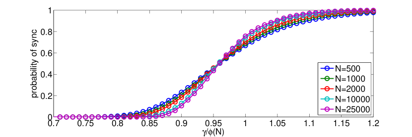
Figure 1: A numerical simulation of the probability of full synchrony in the Kuramoto model in the newly identified scaling.

Finally we close this section with some numerical simulations. The figure 1 depicts a Monte-Carlo simulation of the Kuramoto problem with $N=1000$, $N=2000$, $N=10,000$ and $N=25,000$ oscillators. The figures were generated as follows: for each realization a direction was generated uniformly on the $N-1$-dimensional sphere, and the distance to the boundary of the stability region was computed. In this situation the formulation of Mirollo and Strogatz was found to be more computationally efficient, and this was solved numerically using a bisection method. For each such direction, given the distance to the stability boundary the conditional probability that a Gaussian random vector in that direction would lie within the stability region could be calculated, and averaging over all realizations gives a numerical approximation to the probability of synchronization. For each of the graphs $5000$ realizations were used.

The numerics agree well with the analytical results. We have shown analytically that in the limit of large $N$ the probability of full synchrony is $0$ for $\gamma<1$. The numerics suggest that

$$\lim_{N\rightarrow\infty}P(\gamma\varphi(N),N)=\left\{\begin{array}[]{c}0\qquad\gamma<\gamma^{*}\\ 1\qquad\gamma>\gamma^{*}\end{array}\right.$$

with a critical coupling constant of roughly $\gamma^{*}\approx 1$. This statement is consistent with, but sharper than, the conclusion of Theorem 4.1.

5 Examples

5.1 Comprehensive example for three oscillators

For $N=3$ there are $2^{3}-2=6$ vertices. The corresponding frequency vectors are given by

$$\vec{\omega}_{1}=(1,1,-2)^{t}$$

$$\vec{\omega}_{2}=(1,-2,1)^{t}$$

$$\vec{\omega}_{3}=(-2,1,1)^{t}$$

$$\vec{\omega}_{4}=(-1,-1,2)^{t}$$

$$\vec{\omega}_{5}=(-1,2,-1)^{t}$$

$$\vec{\omega}_{6}=(2,-1,-1)^{t}.$$

The plane orthogonal to the vector $(1,1,1)$ is spanned by the vectors

$${\bf e}_{1}=(1,0,-1)/\sqrt{2},\quad{\bf e}_{2}=(1,-2,1)/\sqrt{6}.$$

In this basis the frequency vectors have the representations $\pm\sqrt{6}{\bf e}_{2},\sqrt{6}(\pm\frac{\sqrt{3}}{2}{\bf e}_{1}\pm\frac{1}{2}{\bf e}_{2})$, which are obviously the vertices of a regular hexagon of side length $\sqrt{6}.$ As shown in the lemma, these represent local minima of distance on the surface of marginal stability.

The phase diagram for three oscillators is summarized in Figure 3. Since the map from the configuration space ${\mathbb{T}}^{n-1}$ to the frequency space ${\mathbb{R}}^{n-1}$ has degree zero it follows that the number of preimages of a given point $\omega$ (the number of configurations with a given frequency) is even, half of which have positive (reduced) Jacobian determinant and half of which have negative Jacobian determinant. The latter are, of course, always unstable. The former have even index but may not be stable. Outside the shaded region there are no fully synchronized solutions. As one crosses the stability boundary a pair of synchronized solutions are created: one is stable (index zero) and one is unstable (index one). The guaranteed stable region, the image of the cube $[0,\frac{\pi}{2}]^{3}$ under the frequency map, is also plotted: it is a dark curve just inside the stable region.

As shown earlier we can derive expressions for the frequency vectors which are hardest and easiest to synchronize. The hardest vectors to synchronize have $(n-1)$ oscillators traveling together with no phase shift and $1$ oscillator leading (or trailing) by phase $\frac{\pi}{2}.$ These solutions have frequency vectors

$$\boldsymbol{\omega}=(\pm 1,\pm 1,\mp 2)$$

and permutations. These points are marked by the six dots on the boundary. These points lie on a circle of radius $\sqrt{6}$. The solutions which are easiest to synchronize have one oscillator at phase $0$, one leading by $x$ and one trailing by $x$ with corresponding frequency vector

$$\boldsymbol{\omega}=\left(\pm(\sin(x)+\sin(2x)),0,\mp(\sin(x)+\sin(2x))\right)$$

plus permutations. The maximum length frequency vector of this form is attained at

$$x=\arccos(\frac{1}{8}(\sqrt{33}-1))$$

which gives a frequency vector of length

$$|{{\boldsymbol{\omega}}}_{{{\mathsf{max}}}}(3)|=\frac{\sqrt{2}}{16}(3+\sqrt{33})\sqrt{\frac{1}{2}\left(15+\sqrt{33}\right)}\approx 2.49$$

It is interesting that, in the case of three oscillators the stability region is very close to a circle and the phase transition to the fully-synchronized state is quite sharp: there are no fully synchronized solutions for $\omega>\frac{\sqrt{2}}{16}(3+\sqrt{33})\sqrt{\frac{1}{2}\left(15+\sqrt{33}\right)}\approx 2.49$ and all solutions synchronize for $\omega<\sqrt{6}\approx 2.45$, a relative frequency shift of about $1.6\%$.

On the interior of the stability region there are two more secondary bifurcation curves, which look like a pair of curvilinear triangles rotated through angle $\frac{2\pi}{6}$ relative to one another. As one crosses these curves a pair of unstable solutions are created, one of index $1$ and one of index $2$. Thus the frequency plane can be subdivided as follows:

• Region 1: Two solutions, one of index $0$ and one of index $1$.

• Region 2: Four solutions, one of index $0$, two of index $1$, one of index $2$.

• Region 3: Six solutions, one of index $0$, three of index $1$, two of index $2$.

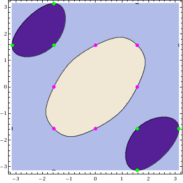
Figure 2: A plot of the stability regions for the three particle system. In the light beige central region the Jacobian is of index 0. In the surrounding pale blue region the Jacobian is of index 1. In the two dark blue islands the Jacobian is of index 2. The marked points depict special points. The six central magenta ones depict the last frequencies to be stabilized, while the six green ones represent points on the boundary between the regions of index 2 and index three.

Also shown is a related figure in the the configuration space. Here the configuration space is colored according to the stability of the given configuration (note that by the $O(1)$ symmetry the first oscillator can be chosen at $\theta_{1}=0$). The light-colored central region represents the stable solutions. It is, as was shown, convex. The surrounding gray region represents the index $1$ solutions, i.e. those with a single unstable direction. Both of these regions cover the range of the frequency map. Finally the two darkest regions represent the two triangular regions where there exist solutions of index two.

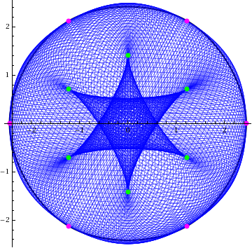
Figure 3: The frequency map. The magenta points correspond to the analogous points in the previous plot: the boundary of the region between the region of index zero and the region of index one corresponds to the boundary of the range. These points denote the last frequency vectors to exhibit synchrony. The green points denote similarly distinguished points on the boundary between the regions of index 1 and index 2. Also shown is the guaranteed stable region, which is tangent to the boundary at the magenta.

5.2 Example for four oscillators

The case of four oscillators is the first with different types of vertices. The vertices are of two types: the first are vertices of the form

$$\vec{\omega}=(\pm 1,\pm 1,\pm 1,\mp 3)$$

and permutations, which have length $\sqrt{12}$. These are local minima of the length of the frequency vector constrained to the surface of marginal stability, and represent the hardest frequencies to stabilize. There are eight such vertices. The second type of vertex has frequency vectors of the form

$$\vec{\omega}=(\pm 2,\pm 2,\mp 2,\mp 2)$$

and permutations, which have length $4$. There are six such vertices and these represent the easiest vectors to stabilize. These points together form the vertices of a polytope known as the rhombic dodecahedron. It is the Voronoi cell for the $A_{3}$ lattice - the face centered cubic lattice.

The figure depicts the region of guaranteed stability - the image of the cube $[0,\frac{\pi}{2}]$ under the frequency projection map. Since this is a symmetric nonlinear projection of the cube in ${\mathbb{R}}^{4}$ into ${\mathbb{R}}^{3}$ it is perhaps not surprising that it takes the form of a curvilinear rhombic dodecahedron, since the corresponding linear projection gives the (flat) rhombic dodecahedron. The vertices typified by the frequency $\omega=(1,1,1,-3)$ are those where three of the curvilinear rhombic faces come together, while those vertices typified by frequencies like $(2,2,-2,-2)$ are those where four rhombic faces meet. The actual stability region (not depicted) is somewhat larger, and resembles an octahedron which is tangent to the region of guaranteed stability at the fourteen vertices listed above.

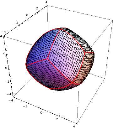
Figure 4: A region of guaranteed stability for the Kuramoto problem with four oscillators. The region is a rhombic dodecahedron with curvilinear faces. The vertices are all points of marginal stability, where there is a zero eigenvalue of multiplicity two or more.

6 Scaling and Extreme Value Statistics

In the preceeding section we showed that the critical scaling for full synchronization differs from the classical scaling by a logarithmic factor: that one should consider

$$\frac{d{\bf\theta}}{dt}={\bf\omega}+\frac{\gamma\sqrt{\log(N^{2})}}{N}$$

rather than the more usual $\frac{1}{N}$ scaling. In this section we give a short heuristic argument as to why this is the correct scaling, which is connected with the extreme value statistics of the frequencies[23, 4].

Let us recall the basics of extreme value statistics. Give a collection of idenpendent and identically distributed random variables $\omega_{i}$ the extreme values statistics concerns the distribution of the quantity $M_{N}=\max(\omega_{1},\omega_{2},\omega_{3},\ldots\omega_{N}).$ The Fisher-Tippett-Gnedenko theorem[23] characterizes the rescaled distribution of such a quantity. It says that if the distribution of a suitably rescaled $M_{N}$ converges to a non-degenerate distribution $G(z)$:

$${\mathbb{P}}(M_{N}-b_{N})/a_{N}\leq z){\rightarrow}G(z)\mbox{ as }{N\rightarrow\infty}$$

then $G(z)$ is one of the following three distributions, the Gumbell, Frechet and Weibull distributions.

$$G_{1}(z) =\exp(\exp(-z)),$$ (6.1)

$$G_{2}(z) =\begin{cases}0,&z\leq 0,\\ \exp(-z^{-\alpha}),&z>0,\\ \end{cases}$$ (6.2)

$$G_{3}(z) =\begin{cases}\exp(-z^{\alpha}),&z<0,\\ 1,&z>0.\end{cases}$$ (6.3)

We claim that the preceeding calculation shows that the probability of full synchrony for the Kuramoto models is bounded above and below by extreme value statistics for the Gaussian, and that the slightly anomolous scaling seen in this problem is a reflection of the extreme value statistics.

It is easy to see that for the Kuramoto problem one has the following obvious estimate for synchronous solutions. From the formula for the frequencies in the classical scaling one has

$$\omega_{i}-\omega_{j}=\frac{1}{N}\sum_{k}\sin(\theta_{k}-\theta_{i})-\sin(\theta_{k}-\theta_{j})$$

leading to the easy estimate

$$\max_{i}(\omega_{i})-\min_{i}(\omega_{i})\leq 2$$

that must hold in order for there to be a fully synchronous solution. This gives an upper bound for the probability in terms of the distribution of

$$\max_{i}(\omega_{i})-\min_{i}(\omega_{i}),$$

a kind of mean adjusted extreme value statistic. This holds for any choice of distribution of the frequencies. For the Gaussian case it is clear that the correct scaling is for this statistic is

$$\max_{i}(\omega_{i})-\min_{i}(\omega_{i})\propto\sqrt{\log{N}}.$$ (6.4)

This gives a motivation for the modified scaling necessary for full synchrony. For Gaussian distibutions of frequencies the lower bound is also of the same form. The lower bound we proved in the preceeding section estimates the probability of synchrony in terms of the probability that the frequency lies in a Voronoi cell of the $A_{N}$ lattice.

So then might pose the question of where the standard scaling might be applicable? We note that the anomalous scaling occurs because of the fact that while the typical sample of a Gaussian is $O(1)$, the maximum of a sample of size $N$ (the first order statistic) is significantly larger than this, being $O(\sqrt{\log N})$. So one could modify the original question: instead of requiring full synchrony for all oscillators, which leads to a condition like (6.4), we could ask the question of whether or not we have “all but one” oscillator synchronize, or even “all but $k$” oscillators synchronize. This would then be governed by the typical size of the second order statistic or the $k+1$st order statistic. However, for fixed $k$ and $N\to\infty$, these all have the same scaling, so we conjecture that for these problems we would also obtain the scaling seen here.

However, if we modified even further and asked for solutions such that some fixed fraction of oscillators synchronized (e.g. for large $N$, we require that $0.9N$ oscillators synchronized), then this would come from the typical size of the 90th percentile of the sample, and this is $O(1)$. Thus we further conjecture that this type of question would lead to the classical scaling. We will consider these questions in future work.

References

• [1] J.A. Acebrรณn, L.L. Bonilla, C.J.P. Vicente, F.ย Ritort, and R.ย Spigler. The Kuramoto model: A simple paradigm for synchronization phenomena. Reviews of modern physics, 77(1):137, 2005.
• [2] Neilย J. Balmforth and Roberto Sassi. A shocking display of synchrony. Phys. D, 143(1-4):21โ€“55, 2000. Bifurcations, patterns and symmetry.
• [3] Matthew Bennett, Michaelย F. Schatz, Heidi Rockwood, and Kurt Wiesenfeld. Huygensโ€™s clocks. R. Soc. Lond. Proc. Ser. A Math. Phys. Eng. Sci., 458(2019):563โ€“579, 2002.
• [4] Eric Bertin and Maxime Clusel. Generalized extreme value statistics and sum of correlated variables. J. Phys. A, 39(24):7607โ€“7619, 2006.
• [5] J.ย H. Conway and N.ย J.ย A. Sloane. Sphere packings, lattices and groups, volume 290 of Grundlehren der Mathematischen Wissenschaften [Fundamental Principles of Mathematical Sciences]. Springer-Verlag, New York, third edition, 1999. With additional contributions by E. Bannai, R. E. Borcherds, J. Leech, S. P. Norton, A. M. Odlyzko, R. A. Parker, L. Queen and B. B. Venkov.
• [6] G.ย Bard Ermentrout. Synchronization in a pool of mutually coupled oscillators with random frequencies. J. Math. Biol., 22(1):1โ€“9, 1985.
• [7] E.ย Fermi, J.ย Pasta, and S.ย Ulam. Studies of nonlinear problems. Los Alamos document LA 1940, 1955.
• [8] J.ย Ford. The Fermi-Pasta-Ulam problem: Paradox turns discovery. Physics Reports, 213(5):271โ€“310, 1992.
• [9] Seung-Yeal Ha, Eunhee Jeong, and Moon-Jin Kang. Emergent behaviour of a generalized Viscek-type flocking model. Nonlinearity, 23(12):3139โ€“3156, 2010.
• [10] Seung-Yeal Ha, Corrado Lattanzio, Bruno Rubino, and Marshall Slemrod. Flocking and synchronization of particle models. Quart. Appl. Math., 69(1):91โ€“103, 2011.
• [11] D.ย Hansel and H.ย Sompolinsky. Synchronization and computation in a chaotic neural network. Phys. Rev. Lett., 68(5):718โ€“721, Feb 1992.
• [12] C.ย Huygens. Horoloquium Oscilatorium. Parisiis, Paris, 1673.
• [13] B.ย W. Knight. Dynamics of encoding in a population of neurons. Journal of General Physiology, 59(6):734โ€“766, 1972.
• [14] N.ย Kopell and G.ย B. Ermentrout. Symmetry and phaselocking in chains of weakly coupled oscillators. Comm. Pure Appl. Math., 39(5):623โ€“660, 1986.
• [15] Y.ย Kuramoto. Chemical oscillations, waves, and turbulence, volumeย 19 of Springer Series in Synergetics. Springer-Verlag, Berlin, 1984.
• [16] Y.ย Kuramoto. Collective synchronization of pulse-coupled oscillators and excitable units. Physica D, 50(1):15โ€“30, May 1991.
• [17] Georgiย S. Medvedev and Nancy Kopell. Synchronization and transient dynamics in the chains of electrically coupled FitzHugh-Nagumo oscillators. SIAM J. Appl. Math., 61(5):1762โ€“1801 (electronic), 2001.
• [18] Renatoย E. Mirollo and Stevenย H. Strogatz. Synchronization of pulse-coupled biological oscillators. SIAM J. Appl. Math., 50(6):1645โ€“1662, 1990.
• [19] Renatoย E. Mirollo and Stevenย H. Strogatz. The spectrum of the locked state for the Kuramoto model of coupled oscillators. Phys. D, 205(1-4):249โ€“266, 2005.
• [20] C.ย S. Peskin. Mathematical aspects of heart physiology. Courant Institute of Mathematical Sciences New York University, New York, 1975. Notes based on a course given at New York University during the year 1973/74, see http://math.nyu.edu/faculty/peskin/heartnotes/index.html.
• [21] A.ย Pikovsky, M.ย Rosenblum, and J.ย Kurths. Synchronization: A Universal Concept in Nonlinear Sciences. Cambridge University Press, 2003.
• [22] Michael Reed and Barry Simon. Methods of modern mathematical physics. IV. Analysis of operators. Academic Press [Harcourt Brace Jovanovich Publishers], New York, 1978.
• [23] Sidneyย I. Resnick. Extreme values, regular variation and point processes. Springer Series in Operations Research and Financial Engineering. Springer, New York, 2008. Reprint of the 1987 original.
• [24] Barry Simon. Spectral analysis of rank one perturbations and applications, 1993. Lectures at the Vancouver Summer School in Mathematical Physics.
• [25] Steven Strogatz. Sync: The Emerging Science of Spontaneous Order. Hyperion, 2003.
• [26] Stevenย H. Strogatz. From Kuramoto to Crawford: exploring the onset of synchronization in populations of coupled oscillators. Phys. D, 143(1-4):1โ€“20, 2000. Bifurcations, patterns and symmetry.
• [27] Dane Taylor, Edward Ott, and Juanย G. Restrepo. Spontaneous synchronization of coupled oscillator systems with frequency adaptation. Phys. Rev. E (3), 81(4):046214, 8, 2010.
• [28] Mark Verwoerd and Oliver Mason. Global phase-locking in finite populations of phase-coupled oscillators. SIAM J. Appl. Dyn. Syst., 7(1):134โ€“160, 2008.
• [29] Mark Verwoerd and Oliver Mason. On computing the critical coupling coefficient for the Kuramoto model on a complete bipartite graph. SIAM J. Appl. Dyn. Syst., 8(1):417โ€“453, 2009.
• [30] Arthurย T. Winfree. The geometry of biological time, volumeย 12 of Interdisciplinary Applied Mathematics. Springer-Verlag, New York, second edition, 2001.