TCD-MATH-11-14 HMI-11-05

Hubbard-Shastry lattice models

Sergey Frolov   and Eoin Quinn

School of Mathematics and Hamilton Mathematics Institute,
Trinity College, Dublin 2, Ireland

Abstract

We consider two lattice models for strongly correlated electrons which are exactly-solvable in one dimension. Along with the Hubbard model and the $\mathfrak{su}(2|2)$ spin chain, these are the only parity-invariant models that can be obtained from Shastry’s R-matrix. One exhibits itinerant ferromagnetic behaviour, while for the other the electrons form bound pairs and at half-filling the model becomes insulating. We derive the TBA equations for the models, analyze them at various limits, and in particular obtain zero temperature phase diagrams. Furthermore we consider extensions of the models, which reduce to the Essler-Korepin-Schoutens model in certain limits.

1 Introduction and Summary

There exist a range of materials whose behaviour is strongly correlated and for which a proper understanding has yet to be established. Prominent in this list are the high-T_c superconductors, itinerant ferromagnets and heavy fermion systems. In this paper we present models which we believe capture some of the features of the first two, and will also briefly comment on a possible connection to the third.

The complete description of a solid is a complex many body problem. Simplifications and exact methods are crucial for progress to be made. In particular, exactly solvable models provide a bedrock on which more realistic models can be constructed and examined. The most important such model is that of free particles. It can be solved in any dimension for both bosons and fermions. The physics of the majority of metals is understood by considering the effects of interaction perturbatively on an exact free solution.

Strongly correlated materials however are those which cannot be understood by reducing the complexity to a non-interacting picture. The collective behaviour of the constituents can drive the material into unexpected phases and interacting exactly solvable models are invaluable for getting insight into such effects. The Hubbard model [2] is a prominent example. Indeed it has become a cornerstone of investigations into strongly correlated electronic behaviour. The model is integrable in one dimension, and describes a Mott insulator [3], which can be seen through its exact solution [4]. The book [5] provides an extensive review of the one-dimensional Hubbard model.

The primary focus of this paper is to investigate two models closely related to the Hubbard model, we call them the A-model and the B-model. Like the Hubbard model they describe spin-1/2 electrons interacting on a lattice and in one dimension can be obtained from Shastry’s R-matrix [6]. For this reason we refer to them as Hubbard-Shastry models, and by construction they are exactly solvable in one dimension. Normally an R-matrix depends on two spectral parameters through their difference, and is thus invariant under shifts of the spectral parameters. Shastry’s R-matrix is special however as it is of a non-difference form and so the actual value of the spectral parameters are important. This was noted in particular by [7, 8], who used this extra variable to construct a one-parameter extension of the Hubbard model. Their extension is hermitian for purely imaginary values of this parameter and is in fact also hermitian along another line for complex values of the parameter. The model is parity invariant however only for special distinct values of the parameter and these correspond, in addition to the Hubbard model, to the A- and B-models, and the $\mathfrak{su}(2|2)$ spin chain.

The A- and B-models have symmetries that are similar to those of the Hubbard model but the phases they exhibit are different. The A-model ground state contains spin-polarised electrons and thus describes itinerant ferromagnetism. For the B-model the electrons form bound pairs and at half-filling it becomes insulating. This is reminiscent of the behaviour of the supersymmetric $t$-$J$ model [9], and has relevance for the modelling of high temperature superconductivity.

The A- and B-models are more involved than the Hubbard model. Both have correlated hopping terms, where the magnitude of the hopping parameters depend on the occupation of the sites by other electrons, and take into account processes such as nearest neighbour Coulomb interaction, spin exchange of two neighbouring electrons of opposite spin, and the pair hopping of two electrons from one site to a neighbouring site. The relative contributions of these terms are strongly constrained by the integrability of the models. Like the Hubbard model they both have one free coupling constant $\mathfrak{u}$ after one normalises the Hamiltonian so that hopping amplitudes are of order 1.

The A-model does not have a free fermion limit, rather the weak coupling $\mathfrak{u}\rightarrow 0$ limit is a model of graded permutations, the $\mathfrak{su}(2|2)$-spin chain [10]. In the strong coupling limit the Hubbard on-site interaction is the dominant term in the Hamiltonian. The model behaves as a ferromagnetic $t$-$J$ model however, in contrast with the antiferromagnetic behaviour of the Hubbard model in this limit.

The B-model does describe free spin-1/2 fermions in the weak coupling limit. As the coupling is increased the hopping becomes correlated and all of the interactions mentioned above begin to contribute. The Hubbard interaction appears in the Hamiltonian but there is no range of $\mathfrak{u}$ for which it is dominant. In the strong coupling limit all terms are of the same order of magnitude, and the model appears to be equivalent to the Essler-Korepin-Schoutens (EKS) model [11] with coupling $U=4$. Furthermore, the model possesses a hidden $\mathfrak{su}(2|2)$ fermionic symmetry for arbitrary coupling.

The integrability of the models is used to study their exact solution in one dimension. As for the Hubbard model, this can be done for arbitrary chemical potential $\mu$ and applied magnetic field $B$. Our formalism allows us to study the Hubbard, A- and B-models in parallel. We restrict our attention to the parameter region $\mu\leq 0$ and $B\geq 0$ (results for the other regions can be obtained using symmetries), here the electron number density ranges from 0 (empty lattice) to 1 (half-filling) and the magnetisation is non-negative. The TBA equations of the models are derived and we analyze them for various limits. Particular focus is paid to obtaining the zero temperature phase diagram in the thermodynamic limit, as this provides the most insight into their properties. Diagonalising the models using the Bethe ansatz technique, taking the thermodynamic limit, and going to zero temperature, the ground states are found to be composed of

• $y$-particles: spin-up electrons,

• $w$-particles: each change the spin of the state by -1,

• $1|vw$-strings: each is a bound state of one spin-up and one spin-down electron.

It is well established [5] that for the Hubbard model there are no $1|vw$-strings in the ground state. In contrast for the B-model there are no $w$-particles, and with no applied magnetic field there are only $1|vw$-strings. The ground state of the A-model is composed only of $y$-particles. The phase diagrams for the A- and B-models are presented in Figure 1. The phases identified are: I. empty band, II. partially filled and spin polarised band, III. half-filled and spin-polarised band, IV. partially filled and partially spin polarised band, V. half-filled and partially spin polarised band.

The ground state of the A-model is spin polarised as it contains only spin-up electrons for $B>0$. The electron number density increases for increasing chemical potential, the lines separating phases I and II and phases II and III depend on the coupling constant respectively as $\mu_{1}=-2-2\sqrt{1+\mathfrak{u}^{2}}-B$ and $\mu_{2}=2-2\sqrt{1+\mathfrak{u}^{2}}-B$. For $B<0$ the phase diagram is mirrored except that here the ground state is polarised with spin-down electrons. Thus we see that the A-model, which describes itinerant electrons on a one-dimensional lattice, is ferromagnetic.

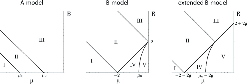
Figure 1: Zero temperature phase diagrams in the $\mu B$-plane for the A- and B- and extended B-models. The phases identified are: I. empty band, II. partially filled and spin polarised band, III. half-filled and spin-polarised band, IV. partially filled and partially spin polarised band, V. half-filled and partially spin polarised band. The dependence of $\mu_{0},\mu_{1},\mu_{2}$ on $\mathfrak{u}$ is given in the text, $\mu_{c}=-2+2\log 2$, and $\mathfrak{g}$ is the coupling constant of the extended B-model.

The phase diagram of the B-model is richer. In the weak coupling limit the point $\mu_{0}$, whose dependence on $\mathfrak{u}$ is given by eq.(6.6), approaches 0, phase V shrinks to a portion of the $B$-axis, and the phase diagram reduces to that of free electrons just as the Hamiltonian does. As the coupling constant is increased to its strong coupling limit the point $\mu_{0}$ decreases monotonically to the value $\mu_{c}=-2+2\log 2\approx-0.6137$. Let us first examine the phase diagram as $\mu$ increases along the line $B=0$. Here the ground state has zero magnetisation and contains only bound pairs of spin-up and spin-down electrons (the $1|vw$-strings). For $\mu<-2$ the cost of having particles in the ground state is too high and the band is empty. The ground state then fills up with the $1|vw$-strings as $\mu$ is increased from $-2$ to $\mu_{0}$, and so is a liquid of singlet pairs. When $\mu$ reaches $\mu_{0}$ the ground state is half-filled and remains half-filled for a range of $\mu$. Thus a gap opens for charge excitations of the ground state and phase V is insulating. Consider now $B>0$. As $B$ is increased spin-up electrons enter the ground state and the model becomes magnetised. This increases the value of $\mu$ that separates phases IV and V and eventually spin-polarises the model, breaking up all of the bound pairs.

It is possible to extend both the A- and B-models by adding the Hubbard interaction term to their Hamiltonians. This decouples the Hubbard interaction from the other terms and in particular for the B-model it allows strong onsite Coulomb repulsion of electrons to be introduced. When the extension dominates the B-model reduces to the $t$-$J$ model with coupling $J$ interpolating between $0$ and $2$ as $\mathfrak{u}$ changes from 0 to $\infty$.

In general the extension destroys the integrability of the models but it happens that there are special values of the coupling constant $\mathfrak{u}$ for which it does not. If $\mathfrak{u}=0$ the extended B-model is just the Hubbard model. In addition the EKS model for arbitrary $U$ can be obtained from the B-model when the coupling constant goes to infinity. Similarly the extended A-model reduces to the EKS model up to the sign of the Hamiltonian after taking $\mathfrak{u}$ to 0. Our formalism can be naturally adapted to the EKS model, and we derive the simplified TBA equations and analyze the zero temperature phase diagram including the dependence on applied magnetic field, see Figure 1.

The plan of the paper is as follows. In section 2 the models are introduced on the level of Hamiltonians and their symmetries are presented. The Bethe equations for the Hubbard-Shastry models are discussed in section 3, and the parity invariant models are identified. Section 4 outlines our formalism for the TBA analysis of the thermodynamic properties of the models, in particular the string hypothesis is formulated, and the TBA equations and free energy are presented. In section 5 we investigate the TBA equations in various limits, namely the weak coupling, strong coupling, strong magnetic field, large chemical potential and infinite temperature limits. The zero temperature limit is discussed in detail in section 6 where the phase diagrams for the A- and B-models are obtained. In section 7 the integrable extensions of the A- and B-models, equivalent to the EKS model, are studied. In Conclusion we discuss future directions. In the appendix A.1 our conventions, definitions and notations are summarised. The derivation of the free energy and the canonical and simplified TBA equations is outlined in appendix A.2. The relation between repulsive and attractive models is discussed in appendix A.3 on the level of the TBA equations. The algebraic limit of the TBA equations is solved in appendix A.4. Finally in appendix A.5 the effect of strong Hubbard interaction on the A-model and the extended B-model is shown to give respectively the ferromagnetic and antiferromagnetic $t$-$J$ models.

2 Lattice models based on Shastry’s R-matrix

2.1 The Hubbard model

The one-dimensional Hubbard model describes spin-1/2 electrons propagating along a lattice with the following nearest-neighbour Hamiltonian

$${\mathbf{H}} = \sum_{j=1}^{L}\,{\mathbf{H}}_{j,j+1}=\sum_{j=1}^{L}\,\left({\mathbf{T}}_{j,j+1}+4\,\mathfrak{u}\,{\mathbf{V}}^{H}_{j,j+1}\right)\,,$$ (2.1)

where $L$ is the length of the chain and the kinetic (hopping) and potential terms are given by

$${\mathbf{T}}_{j,k} = -\sum_{\sigma=\uparrow,\downarrow}\big{(}{\mathbf{c}}^{\dagger}_{j,\sigma}\mathbf{c}_{k,\sigma}+{\mathbf{c}}^{\dagger}_{k,\sigma}\mathbf{c}_{j,\sigma}\big{)}\,,$$ (2.2)

$${\mathbf{V}}^{H}_{j,k} = {1\over 2}\,\big{(}\mathbf{n}_{j,\uparrow}-{1\over 2}\big{)}\big{(}\mathbf{n}_{j,\downarrow}-{1\over 2}\big{)}+{1\over 2}\,\big{(}\mathbf{n}_{k,\uparrow}-{1\over 2}\big{)}\big{(}\mathbf{n}_{k,\downarrow}-{1\over 2}\big{)}-{1\over 4}\,.$$ (2.3)

Here the canonically anticommuting fermionic operators ${\mathbf{c}}^{\dagger}_{j,\sigma}$ create and $\mathbf{c}_{j,\sigma}$ annihilate electrons of spin $\sigma=\uparrow$ or $\sigma=\downarrow$ at the $j$-th site of the lattice. The operator $\mathbf{n}_{j,\sigma}={\mathbf{c}}^{\dagger}_{j,\sigma}\mathbf{c}_{j,\sigma}$ is the local particle number operator for electrons of spin $\sigma$ at site $j$, and in what follows we also use $\mathbf{n}_{j}=\mathbf{n}_{j,\uparrow}+\mathbf{n}_{j,\downarrow}$. The coupling constant $\mathfrak{u}$ is $\mathfrak{u}=U/4t$, and the hopping parameter $t$ is set to 1. We also assume that $\mathfrak{u}$ is positive.

The Hamiltonian (2.1) is very symmetric. Beyond possessing parity and translational invariance it is invariant under a spin $\mathfrak{su}(2)$ and a charge $\mathfrak{su}(2)$, the generators of which are given respectively by

$$\begin{array}[]{cclcclccl}{\mathbf{S}}^{+}&=&\sum_{j=1}^{L}{\mathbf{S}}_{j}^{+}\,,&{\mathbf{S}}^{-}&=&\sum_{j=1}^{L}{\mathbf{S}}_{j}^{-}\,,&{\mathbf{S}}^{z}&=&\sum_{j=1}^{L}{\mathbf{S}}_{j}^{z}\,,\vspace{0.2cm}\\ {\boldsymbol{\eta}}^{+}&=&\sum_{j=1}^{L}(-1)^{j}{\boldsymbol{\eta}}_{j}^{+}\,,&{\boldsymbol{\eta}}^{-}&=&\sum_{j=1}^{L}(-1)^{j}{\boldsymbol{\eta}}_{j}^{-}\,,&{\boldsymbol{\eta}}^{z}&=&\sum_{j=1}^{L}{\boldsymbol{\eta}}_{j}^{z}\,.\end{array}$$ (2.4)

where

$$\begin{array}[]{cclcclccl}{\mathbf{S}}_{j}^{+}&=&{\mathbf{c}}^{\dagger}_{j,\uparrow}\mathbf{c}_{j,\downarrow},&{\mathbf{S}}_{j}^{-}&=&{\mathbf{c}}^{\dagger}_{j,\downarrow}\mathbf{c}_{j,\uparrow},&{\mathbf{S}}_{j}^{z}&=&\frac{1}{2}(\mathbf{n}_{j,\uparrow}-\mathbf{n}_{j,\downarrow})\,,\vspace{0.2cm}\\ {\boldsymbol{\eta}}_{j}^{+}&=&{\mathbf{c}}^{\dagger}_{j,\downarrow}{\mathbf{c}}^{\dagger}_{j,\uparrow},&{\boldsymbol{\eta}}_{j}^{-}&=&\mathbf{c}_{j,\uparrow}\mathbf{c}_{j,\downarrow},&{\boldsymbol{\eta}}_{j}^{z}&=&\frac{1}{2}(\mathbf{n}_{j}-1)\,.\end{array}$$ (2.5)

Often one considers the more general Hamiltonian

$${\mathbf{H}}-\mu\,{\mathbf{N}}-2\,B\,{\mathbf{S}}^{z}$$ (2.6)

with ${\mathbf{N}}=\sum_{j=1}^{L}\mathbf{n}_{j}=2{\boldsymbol{\eta}}^{z}+L$. The chemical potential $\mu$ and magnetic field $B$ break the charge and spin $\mathfrak{su}(2)$ respectively, leaving only the two $\mathfrak{u}(1)$ subalgebras unbroken as $[{\mathbf{H}},{\mathbf{N}}]=0$ and $[{\mathbf{H}},{\mathbf{S}}^{z}]=0$. Note that

$${\mathbf{V}}^{\rm H}\equiv\sum_{j=1}^{L}\,{\mathbf{V}}^{H}_{j,j+1}=\sum_{j=1}^{L}\,\mathbf{n}_{j,\uparrow}\mathbf{n}_{j,\downarrow}-{1\over 2}{\bf N}\,.$$ (2.7)

The Hubbard Hamiltonian is most commonly presented in a form that hides the charge $\mathfrak{su}(2)$ symmetry with $\mu=-2\mathfrak{u}$ and $B=0$ in (2.6).

There have been various attempts to extend the Hubbard model by introducing correlated hopping and adding various extra terms to the interaction of the Hamiltonian (also by introducing next-nearest-neighbour hopping but this shall not be considered here). In general one would expect these to explicitly break the symmetries of the model. It is also possible however that certain extensions realise different symmetries, e.g. [11]-[16], and we see this below in the A- and B-models.

2.2 Construction

The Hubbard-Shastry Hamiltonian can be obtained by using Shastry’s R-matrix [6] and the standard techniques of integrable spin chains [17, 5]. It was found recently [18] that Shastry’s R-matrix is equivalent to the $\mathfrak{su}(2|2){{}_{\cal C}}$-invariant R-matrix [19] which appears as a building block of the ${\rm AdS}_{5}\times{\rm S}^{5}$ scattering S-matrix playing an important role in the AdS/CFT spectral problem, see [20, 21] for a review. Moreover, the $\mathfrak{su}(2|2){{}_{\cal C}}$ invariance together with the physical unitarity condition is sufficient to fix an R-matrix satisfying the Yang-Baxter equation up to a phase [19].

The Hilbert space for each site of the one dimensional Hubbard model is a four dimensional graded vector space because a site can be either empty or doubly occupied, or can have a single electron of either spin. The fundamental representation of $\mathfrak{su}(2|2){{}_{\cal C}}$ is also a four dimensional graded vector space ${\mathscr{V}}$, see [18] for detail. The Hilbert space for the model on a lattice of length $L$ is thus naturally identified with $\otimes_{j=1}^{L}{\mathscr{V}}_{j}$:

$$|0\rangle\leftrightarrow|e_{j,1}\rangle,\quad{\mathbf{c}}^{\dagger}_{j,\uparrow}{\mathbf{c}}^{\dagger}_{j,\downarrow}|0\rangle\leftrightarrow|e_{j,2}\rangle,\quad{\mathbf{c}}^{\dagger}_{j,\uparrow}|0\rangle\leftrightarrow|e_{j,3}\rangle,\quad{\mathbf{c}}^{\dagger}_{j,\downarrow}|0\rangle\leftrightarrow|e_{j,4}\rangle\,.$$ (2.8)

The identification is not unique as one can perform canonical transformations on $\mathbf{c}_{j,\sigma}\,,{\mathbf{c}}^{\dagger}_{j,\sigma}$.

A representation of $\mathfrak{su}(2|2){{}_{\cal C}}$ depends on the values of the central elements. These can be conveniently parametrized by variables $x^{\pm}$ satisfying

$$x^{+}+\frac{1}{x^{+}}-x^{-}-\frac{1}{x^{-}}=4\,i\,\mathfrak{u}\,.$$ (2.9)

The constraint defines a torus with $\mathfrak{u}$ a free parameter that characterises its elliptic modulus and that we will interpret as a coupling constant. Indeed in the setting where one obtains the Hubbard model this is precisely the coupling constant that appears in the Hubbard Hamiltonian (2.1). The $\mathfrak{su}(2|2){{}_{\cal C}}$-invariant R-matrix ${\mathbf{R}}(x^{\pm}_{1},x^{\pm}_{2})$ depends on two spectral parameters which from the point of view of the $\mathfrak{su}(2|2){{}_{\cal C}}$ algebra parametrize the two 4-dim fundamental representations upon which the R-matrix acts. We restrict our attention to homogeneous spin chains, that the variables $x^{\pm}$ of each of the representations of $\mathfrak{su}(2|2){{}_{\cal C}}$ comprising the chain are the same at each site. Then $x^{\pm}$ play the role of extra coupling constants of the model and the density of the nearest neighbour Hubbard-Shastry Hamiltonian is obtained in the standard way through the formula

$${\mathbf{H}}_{j,j+1}\sim i\,{\mathbf{P}}_{j,j+1}\partial_{1}{\mathbf{R}}_{j,j+1}(x^{\pm}_{1},x^{\pm})|_{x^{\pm}_{1}=x^{\pm}}\,,$$ (2.10)

where ${\mathbf{P}}_{j,j+1}$ is the permutation matrix, see appendix A.1 for precise definitions.

Any point $x^{\pm}$ on the torus can be used to obtain a homogeneous integrable spin chain model. In general however the corresponding Hamiltonian will be neither hermitian nor parity invariant. One can show by using the properties of the R-matrix that it is hermitian if either $x^{+}/x^{-}$ or $x^{+}x^{-}$ is a phase. In the next section we examine the Bethe equations of the models and find that there are just four distinct points on the torus, up to symmetries, that give rise to hermitian parity invariant models. The Hubbard model is obtained when $x^{-}=1/x^{+}$. Two of the models have not been singled out before, one at $x^{-}=-1/x^{+}$ which we call the A-model, and one at $x^{-}=-x^{+}$ which we call the B-model. Completing the picture is the point $x^{-}=x^{+}$. Here the central extension of the algebra vanishes and one obtains the $\mathfrak{su}(2|2)$ spin chain. It is singular from our perspective as the coupling $\mathfrak{u}$ drops out.

Given a Hamiltonian one can study either the model determined by ${\mathbf{H}}$ or $-{\mathbf{H}}$. For example instead of the Hubbard model one could consider

$${\mathbf{H}}^{\rm attr.H}=\sum_{j=1}^{L}\,\left(-{\mathbf{T}}_{j,j+1}-4\,\mathfrak{u}\,{\mathbf{V}}^{H}_{j,j+1}\right)\,.$$ (2.11)

This is the attractive Hubbard model and its physical properties are very different from the repulsive case, see e.g. [5]. For the A- and B-models, which were constructed not on physical grounds but to have rich symmetry and act on the Hubbard lattice, one has a choice for the sign of the Hamiltonian. With the hope that they capture some interesting physics the sign is chosen so that there is a cost for a doubly occupied site relative to a singly occupied site, mirroring Coulomb repulsion. Note however that although properties depend strongly on the choice of sign the two cases are closely related. This is discussed in appendix A.3 at the level of the TBA equations.

Let us comment on the sign of the kinetic term in (2.11). Under the unitary transformation generated by

$${\mathbf{U}}_{1}(\alpha)=\exp\Big{(}i\,\alpha\,\sum_{j=1}^{L}j\,(\mathbf{n}_{j,\uparrow}+\mathbf{n}_{j,\downarrow})\Big{)}$$ (2.12)

with $\alpha$ an arbitrary real parameter, the kinetic term transforms as ($k=j+1$)

$${\mathbf{T}}_{j,k}\rightarrow{\mathbf{U}}_{1}^{\dagger}(\alpha){\mathbf{T}}_{j,k}{\mathbf{U}}_{1}(\alpha)=-\sum_{\sigma=\uparrow\downarrow}\big{(}e^{i\alpha}{\mathbf{c}}^{\dagger}_{j,\sigma}\mathbf{c}_{k,\sigma}+e^{-i\alpha}{\mathbf{c}}^{\dagger}_{k,\sigma}\mathbf{c}_{j,\sigma}\big{)}$$ (2.13)

while the interaction ${\mathbf{V}}^{H}$ is invariant. Thus the Hamiltonian (2.11) is unitary equivalent to

$$\sum_{j=1}^{L}\,\left({\mathbf{T}}_{j,j+1}-4\,\mathfrak{u}\,{\mathbf{V}}^{H}_{j,j+1}\right)\,$$ (2.14)

under ${\mathbf{U}}_{1}(\pi)$. In momentum space $\sum_{j=1}^{L}\,{\mathbf{T}}_{j,j+1}$ is diagonalised as $-2\sum_{p}\cos p\,(\mathbf{n}_{p,\uparrow}+\mathbf{n}_{p,\downarrow})$ and the transformation ${\mathbf{U}}_{1}(\alpha)$ corresponds to a shift $p\rightarrow p^{\prime}=p+\alpha$. This is why the attractive Hubbard model is conventionally written as (2.14), as states with $p^{\prime}=0$ then minimize the kinetic part of the Hamiltonian. In general for a Hamiltonian ${\mathbf{H}}$ we define the Hamiltonian $\widetilde{\mathbf{H}}$ which has the opposite spectrum

$$\widetilde{\mathbf{H}}=-{\mathbf{U}}_{1}^{\dagger}(\pi)\,{\mathbf{H}}\,{\mathbf{U}}_{1}(\pi).$$ (2.15)

For this reason in what follows we refer to $\widetilde{\mathbf{H}}$ as the opposite Hamiltonian.

The direct calculation from the R-matrix at $x^{-}=1/x^{+}$ does not give the Hubbard Hamiltonian (2.1) but rather one must perform the unitary transformation generated by ${\mathbf{U}}_{1}(-\pi/2)$ to obtain it, which also twists the charge $\mathfrak{su}(2)$ generators. To obtain the Hamiltonians for the A- and B-models (2.3, 2.19) one must apply ${\mathbf{U}}_{1}(\pi)$ and ${\mathbf{U}}_{1}(-\pi/2)$ respectively to the corresponding results from the R-matrix calculation. These twists can be understood also at the level of the Bethe equations, see the relations (3.5).

2.3 The A- and B-models

Both the A- and B-models have correlated hopping kinetic terms and we will discuss these soon in turn. The interactions of the models are combinations of several common terms. In addition to the Hubbard interaction ${\mathbf{V}}^{H}$, these are

$${\mathbf{V}}_{j,k}^{CC} = \,{\boldsymbol{\eta}}_{j}^{z}\,{\boldsymbol{\eta}}_{k}^{z}-\frac{1}{4}\ =\ \frac{1}{4}\left(\mathbf{n}_{j}-1)(\mathbf{n}_{k}-1\right)-\frac{1}{4}\ \,,$$

$${\mathbf{V}}_{j,k}^{SS} = \frac{1}{2}({\mathbf{S}}_{j}^{+}\,{\mathbf{S}}_{k}^{-}+{\mathbf{S}}_{j}^{-}\,{\mathbf{S}}_{k}^{+})+{\mathbf{S}}_{j}^{z}\,{\mathbf{S}}_{k}^{z}$$

$$= \frac{1}{2}({\mathbf{c}}^{\dagger}_{j,\uparrow}\mathbf{c}_{j,\downarrow}{\mathbf{c}}^{\dagger}_{k,\downarrow}\mathbf{c}_{k,\uparrow}+{\mathbf{c}}^{\dagger}_{j,\downarrow}\mathbf{c}_{j,\uparrow}{\mathbf{c}}^{\dagger}_{k,\uparrow}\mathbf{c}_{k,\downarrow})+\frac{1}{4}\left(\mathbf{n}_{j,\uparrow}-\mathbf{n}_{j,\downarrow}\right)\left(\mathbf{n}_{k,\uparrow}-\mathbf{n}_{k,\downarrow}\right)\,,$$

$${\mathbf{V}}_{j,k}^{PH} = \frac{1}{2}({\boldsymbol{\eta}}_{j}^{+}\,{\boldsymbol{\eta}}_{k}^{-}+{\boldsymbol{\eta}}_{j}^{-}\,{\boldsymbol{\eta}}_{k}^{+})\ =\ \frac{1}{2}({\mathbf{c}}^{\dagger}_{j,\uparrow}{\mathbf{c}}^{\dagger}_{j,\downarrow}\mathbf{c}_{k,\downarrow}\mathbf{c}_{k,\uparrow}+{\mathbf{c}}^{\dagger}_{k,\uparrow}{\mathbf{c}}^{\dagger}_{k,\downarrow}\mathbf{c}_{j,\downarrow}\mathbf{c}_{j,\uparrow})\,.$$

The charge-charge interaction ${\mathbf{V}}^{CC}$ has the interpretation of nearest neighbour Coulomb repulsion. Physically one should think of a site as having charge +1, and so a site with one electron on it has neutral charge, a site with electron density less than one is positively charged and a site with electron density greater than one is negatively charged. The spin-spin interaction ${\mathbf{V}}^{SS}$ is the familiar spin-exchange term of the Heisenberg XXX spin chain. Finally the pair hopping interaction ${\mathbf{V}}^{PH}$ relates to the simultaneous hopping of two electrons from one site to a neighbouring site.

Now we discuss the A- and B-models in turn. The presentation of the Hamiltonians is much cleaner if the coupling constant $\mathfrak{u}$ is re-expressed through

$$\mathfrak{u}=\sinh\nu\,.$$

A-model

The model at $x^{+}x^{-}=-1$ has the Hamiltonian

$${\mathbf{H}}^{\rm A} = \sum_{j=1}^{L}\,\Big{(}{\mathbf{T}}_{j,j+1}^{\rm A}+\frac{2\cosh 2\nu}{\cosh\nu}\,{\mathbf{V}}^{H}_{j,j+1}+{2\over\cosh\nu}\,\big{(}{\mathbf{V}}_{j,j+1}^{CC}-{\mathbf{V}}_{j,j+1}^{SS}+{\mathbf{V}}_{j,j+1}^{PH}\big{)}\Big{)}\,,~{}~{}~{}~{}~{}~{}$$

$${\mathbf{T}}_{j,k}^{\rm A} = -\sum_{\sigma}\Big{[}\big{(}{\mathbf{c}}^{\dagger}_{j,\sigma}\mathbf{c}_{k,\sigma}+{\mathbf{c}}^{\dagger}_{k,\sigma}\mathbf{c}_{j,\sigma}\big{)}\big{(}1-\mathbf{n}_{j,-\sigma}-\mathbf{n}_{k,-\sigma}\big{)}$$

$$\qquad\qquad-i\tanh\nu\big{(}{\mathbf{c}}^{\dagger}_{j,\sigma}\mathbf{c}_{k,\sigma}-{\mathbf{c}}^{\dagger}_{k,\sigma}\mathbf{c}_{j,\sigma}\big{)}\big{(}\mathbf{n}_{j,-\sigma}-\mathbf{n}_{k,-\sigma}\big{)}^{2}{\Big{]}}.$$

It is easy to check that it is hermitian but its parity invariance is more subtle. Note that the transformation

$${\mathbf{c}}^{\dagger}_{j,\sigma}\rightarrow{\mathbf{c}}^{\dagger}_{L-j+1,\sigma}\,,\qquad\mathbf{c}_{j,\sigma}\rightarrow\mathbf{c}_{L-j+1,\sigma}\,,$$ (2.17)

is not a symmetry but is instead equivalent to a replacement $\nu\rightarrow-\nu$ in the Hamiltonian. This however is just a unitary transformation. More generally, the Hamiltonian (2.3) is unitary equivalent to the following one

$${\mathbf{H}}^{\rm A}(\alpha) \equiv {\mathbf{U}}_{2}^{\dagger}(\alpha)\,{\mathbf{H}}^{\rm A}\,{\mathbf{U}}_{2}(\alpha)\,,\quad{\mathbf{U}}_{2}(\alpha)\equiv\exp\left(i\,\alpha\,\sum_{j=1}^{L}\mathbf{n}_{j,\uparrow}\mathbf{n}_{j,\downarrow}\right)\,,$$

$${\mathbf{H}}^{\rm A}(\alpha) = \sum_{j=1}^{L}\,\Big{(}{\mathbf{T}}_{j,j+1}^{\rm A}(\alpha)+\frac{2\cosh 2\nu}{\cosh\nu}\,{\mathbf{V}}^{H}_{j,j+1}+{2\over\cosh\nu}\,\big{(}{\mathbf{V}}_{j,j+1}^{CC}-{\mathbf{V}}_{j,j+1}^{SS}+{\mathbf{V}}_{j,j+1}^{PH}\big{)}\Big{)}\,,$$

$${\mathbf{T}}_{j,k}^{\rm A}(\alpha) = -\sum_{\sigma}\Big{[}\big{(}{\mathbf{c}}^{\dagger}_{j,\sigma}\mathbf{c}_{k,\sigma}+{\mathbf{c}}^{\dagger}_{k,\sigma}\mathbf{c}_{j,\sigma}\big{)}\big{(}1-\mathbf{n}_{j,-\sigma}-\mathbf{n}_{k,-\sigma}-\sin\alpha\tanh\nu\,(\mathbf{n}_{j,-\sigma}-\mathbf{n}_{k,-\sigma})\big{)}$$ (2.18)

$$\qquad\qquad-i\cos\alpha\tanh\nu\big{(}{\mathbf{c}}^{\dagger}_{j,\sigma}\mathbf{c}_{k,\sigma}-{\mathbf{c}}^{\dagger}_{k,\sigma}\mathbf{c}_{j,\sigma}\big{)}\big{(}\mathbf{n}_{j,-\sigma}-\mathbf{n}_{k,-\sigma}\big{)}^{2}{\Big{]}}\,,$$

where $\alpha$ is an arbitrary real parameter. If one chooses $\alpha=\pi$ one gets

$${\mathbf{H}}^{\rm A}(\pi)={\mathbf{H}}^{\rm A}\ \ {\rm with}\ \ \nu\to-\nu\,,$$

and so the parity transformation (2.17) should be supplemented with the change of basis generated by ${\mathbf{U}}_{2}(\pi)$. Note also that with the choice $\alpha=\pm\pi/2$ one removes the imaginary term from the Hamiltonian.

The kinetic part of the Hamiltonian is of a complicated correlated hopping type. It is instructive to see how it acts in various cases. For an electron of spin $\sigma$ to hop between two sites $j$ and $k$ they must not contain other electrons of that spin but they can contain electrons of the opposite spin. We consider individually the four possibilities as illustrated in Figure 2 for a mobile spin-up electron. The kinetic density ${\mathbf{T}}_{j,k}^{\rm A}(\alpha)$ acting on each of the cases takes the form

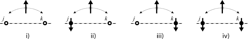
Figure 2: The four cases of an electron hopping between sites $j$ and $k$: i) no electrons of the opposite spin on either site, ii) an electron of the opposite spin on site $j$ only, iii) an electron of the opposite spin on site $k$ only, iv) electrons of the opposite spin on both sites.

1. i)     $-{\mathbf{c}}^{\dagger}_{j,\sigma}\mathbf{c}_{k,\sigma}-\,{\mathbf{c}}^{\dagger}_{k,\sigma}\mathbf{c}_{j,\sigma}$,

2. ii)     $-ie^{-i\alpha}\tanh\nu\,{\mathbf{c}}^{\dagger}_{j,\sigma}\mathbf{c}_{k,\sigma}+ie^{i\alpha}\tanh{\nu}\,{\mathbf{c}}^{\dagger}_{k,\sigma}\mathbf{c}_{j,\sigma}$,

3. iii)     $-ie^{i\alpha}\tanh\nu\,{\mathbf{c}}^{\dagger}_{j,\sigma}\mathbf{c}_{k,\sigma}+ie^{-i\alpha}\tanh{\nu}\,{\mathbf{c}}^{\dagger}_{k,\sigma}\mathbf{c}_{j,\sigma}$,

4. iv)     ${\mathbf{c}}^{\dagger}_{j,\sigma}\mathbf{c}_{k,\sigma}+\,{\mathbf{c}}^{\dagger}_{k,\sigma}\mathbf{c}_{j,\sigma}$.

Note the different sign between cases i) and iv), while in the case of free electrons all the cases would be the same as case i). This reflects the strong electron correlation in the A-model which cannot be reduced to free electrons for any coupling.

Like all the models we consider, the A-model inherits spin and charge $\mathfrak{su}(2)$ symmetries from the $\mathfrak{su}(2|2){{}_{\cal C}}$ structure. The spin $\mathfrak{su}(2)$ generators take the same form as those for the Hubbard model (2.4) whereas the charge $\mathfrak{su}(2)$ generators take a untwisted form.

The weak coupling $\nu\rightarrow 0$ limit of the A-model is not described by free electrons but rather the Hamiltonian reduces to the ${\mathfrak{su}(2|2)}$ spin chain. This has received much study due to an interesting generalisation found in [11]. A key observation is that ${\mathbf{V}}^{\rm H}$ commutes with ${\mathbf{H}}^{\rm A}\big{|}_{\nu=0}$ and so one can extend the model, as will be discussed in section 2.4. In the strong coupling $\nu\rightarrow\infty$ limit only the term $4\,\mathfrak{u}{\mathbf{V}}^{\rm H}$ in the Hamiltonian survives and it thus shares the strict strong coupling limit of the Hubbard model. In section 5.2 we show that at half-filling and strong coupling the model behaves as a ferromagnetic XXX spin chain. The strong coupling limit of the less than half-filled model is analysed in appendix A.5 and is found to be a ferromagnetic t-J model.

B-model

The model at $x^{+}/x^{-}=-1$ has the Hamiltonian

$${\mathbf{H}}^{\rm B} = \sum_{j=1}^{L}\,\Big{(}{\mathbf{T}}_{j,j+1}^{\rm B}+2\tanh\nu\,\big{(}{\mathbf{V}}_{j,j+1}^{H}-{\mathbf{V}}_{j,j+1}^{CC}+{\mathbf{V}}_{j,j+1}^{SS}+{\mathbf{V}}_{j,j+1}^{PH}\big{)}\Big{)}\,,$$ (2.19)

$${\mathbf{T}}_{j,k}^{\rm B} = -\sum_{\sigma}\big{(}{\mathbf{c}}^{\dagger}_{j,\sigma}\mathbf{c}_{k,\sigma}+{\mathbf{c}}^{\dagger}_{k,\sigma}\mathbf{c}_{j,\sigma}\big{)}\Big{(}1-\big{(}1-{1\over\cosh\nu}\big{)}\big{(}\mathbf{n}_{j,-\sigma}-\mathbf{n}_{k,-\sigma}\big{)}^{2}\Big{)}.$$

Let us begin the analysis by examining the correlated hopping kinetic term for the four cases illustrated in Figure 2. The model is clearly parity invariant and so cases ii) and iii) are identical. The kinetic density ${\mathbf{T}}_{j,k}^{\rm B}(\alpha)$ acting on each of the cases takes the form

• i), iv)     $-{\mathbf{c}}^{\dagger}_{j,\sigma}\mathbf{c}_{k,\sigma}-\,{\mathbf{c}}^{\dagger}_{k,\sigma}\mathbf{c}_{j,\sigma}$,

• ii), iii)      $-{1\over\cosh\nu}({\mathbf{c}}^{\dagger}_{j,\sigma}\mathbf{c}_{k,\sigma}+\,{\mathbf{c}}^{\dagger}_{k,\sigma}\mathbf{c}_{j,\sigma})$.

In cases i) and iv) hopping is of the standard form, while in cases ii) and iii) its contribution is proportional to $\mbox{sech}\,\nu$ and decreases to zero in the strong coupling limit. Both cases i) and iv) preserve the number of doubly occupied sites, while for hopping in cases ii) and iii) the number will be either increased or decreased by 1.

The B-model describes free electrons in the weak coupling $\nu\rightarrow 0$ limit. In the strong coupling $\nu\rightarrow\infty$ limit note that $[{\mathbf{H}}^{\rm B}\,,{\mathbf{V}}^{\rm H}]=0$, as for the weak coupling limit of the A-model. This allows one to decouple the coefficient of the Hubbard interaction from the other terms while preserving the integrability, see section 2.4.

The B-model possesses a rich symmetry structure. Its spin and charge $\mathfrak{su}(2)$ generators take the same form as for the Hubbard model (2.4). Moreover the model inherits a hidden $\mathfrak{su}(2|2)$ fermionic symmetry for arbitrary coupling constant $\nu$ from Shastry’s R-matrix. There are eight supercharges, four of which ${\mathbf{Q}}^{\dagger}_{0,\sigma}$, ${\mathbf{Q}}_{0,\sigma}$ create/annihilate an electron with momentum $p=0$, and the other four ${\mathbf{Q}}^{\dagger}_{\pi,\sigma}$, ${\mathbf{Q}}_{\pi,\sigma}$ create/annihilate an electron with momentum $p=\pi$. Explicitly they are

$${\mathbf{Q}}_{\alpha,\sigma} = \sum_{j=1}^{L}e^{i\,\alpha\,j}(\gamma_{\alpha}\,\mathbf{c}_{j,\sigma}-\beta\,\mathbf{n}_{j,-\sigma}\mathbf{c}_{j,\sigma})\,,\quad{\mathbf{Q}}^{\dagger}_{\alpha,\sigma}=({\mathbf{Q}}_{\alpha,\sigma})^{\dagger}\,,\quad\alpha=0,\pi\,,~{}~{}~{}~{}$$

with $$\gamma_{\alpha}={1\over 2}\left(\beta+{e^{i\,\alpha}\over\beta}\right)\mbox{ and }\beta=\sqrt{\tanh{\nu\over 2}}\,,$$

and they satisfy the $\mathfrak{su}(2|2)$ algebra with central charge $\coth\nu$:

$$\{{\mathbf{Q}}_{0,\downarrow},{\mathbf{Q}}^{\dagger}_{0,\uparrow}\} = -\,\{{\mathbf{Q}}_{\pi,\downarrow},{\mathbf{Q}}^{\dagger}_{\pi,\uparrow}\}\,=\,{\mathbf{S}}^{+}\,,\quad\{{\mathbf{Q}}_{0,\uparrow},{\mathbf{Q}}^{\dagger}_{0,\downarrow}\}\,=\,-\,\{{\mathbf{Q}}_{\pi,\uparrow},{\mathbf{Q}}^{\dagger}_{\pi,\downarrow}\}\,=\,{\mathbf{S}}^{-}\,,$$

$$\{{\mathbf{Q}}^{\dagger}_{0,\downarrow},{\mathbf{Q}}^{\dagger}_{\pi,\uparrow}\} = -\,\{{\mathbf{Q}}^{\dagger}_{0,\uparrow},{\mathbf{Q}}^{\dagger}_{\pi,\downarrow}\}\,=\,{\boldsymbol{\eta}}^{+}\,,\quad\,\{{\mathbf{Q}}_{0,\downarrow},{\mathbf{Q}}_{\pi,\uparrow}\}\,=\,-\,\{{\mathbf{Q}}_{0,\uparrow},{\mathbf{Q}}_{\pi,\downarrow}\}\,=\,{\boldsymbol{\eta}}^{-}\,,$$

$$\{{\mathbf{Q}}_{0,\uparrow},{\mathbf{Q}}^{\dagger}_{0,\uparrow}\} = {\mathbf{S}}^{z}-{\boldsymbol{\eta}}^{z}+\coth\nu\,,\qquad\quad\{{\mathbf{Q}}_{0,\downarrow},{\mathbf{Q}}^{\dagger}_{0,\downarrow}\}\,=\,-\,{\mathbf{S}}^{z}-{\boldsymbol{\eta}}^{z}+\coth\nu\,,$$

$$\{{\mathbf{Q}}_{\pi,\uparrow},{\mathbf{Q}}^{\dagger}_{\pi,\uparrow}\} = -\,{\mathbf{S}}^{z}+{\boldsymbol{\eta}}^{z}+\coth\nu\,,\qquad\,\{{\mathbf{Q}}_{\pi,\downarrow},{\mathbf{Q}}^{\dagger}_{\pi,\downarrow}\}\,=\,{\mathbf{S}}^{z}+{\boldsymbol{\eta}}^{z}+\coth\nu\,,$$

and all other anti-commutators vanish. The symmetry is hidden in that these generators do not commute with the Hamiltonian but rather

$$[{\mathbf{H}^{\rm B}},{\mathbf{Q}}]=h_{Q}\,{\mathbf{Q}}\,,\quad[{\mathbf{N}},{\mathbf{Q}}]=n_{Q}\,{\mathbf{Q}}\,,\quad[{\mathbf{S}}^{z},{\mathbf{Q}}]=s_{Q}\,{\mathbf{Q}}\,,$$

with $h_{Q}$, $n_{Q}$ and $s_{Q}$ given in Table 1.

	${\mathbf{Q}}_{0,\uparrow}$	${\mathbf{Q}}_{0,\downarrow}$	${\mathbf{Q}}_{\pi,\uparrow}$	${\mathbf{Q}}_{\pi,\downarrow}$	${\mathbf{Q}}^{\dagger}_{0,\uparrow}$	${\mathbf{Q}}^{\dagger}_{0,\downarrow}$	${\mathbf{Q}}^{\dagger}_{\pi,\uparrow}$	${\mathbf{Q}}^{\dagger}_{\pi,\downarrow}$
$h_{Q}$	2	2	-2	-2	-2	-2	2	2
$n_{Q}$	-1	-1	-1	-1	1	1	1	1
$s_{Q}$	-1/2	1/2	-1/2	1/2	1/2	-1/2	1/2	-1/2

Table 1: Commutators of supercharges of the B-model with $\mathbf{H}$, $\mathbf{N}$ and $\mathbf{S}^{z}$.

Thus the symmetry does not lead to an extra degeneracy in the spectrum of the model, but it does imply exact relationships between the energies of eigenstates. For example if $|\psi\rangle$ is an eigenstate with energy $\mathcal{E}_{\psi}$, then the energy of the state ${\mathbf{Q}}|\psi\rangle$ is given through ${\mathbf{H}}^{\rm B}{\mathbf{Q}}|\psi\rangle=(\mathcal{E}_{\psi}+h_{Q}){\mathbf{Q}}|\psi\rangle$. In particular it follows that the ground state of ${\mathbf{H}}^{\rm B}$ is in the kernel of ${\mathbf{Q}}^{\dagger}_{0,\uparrow}$, ${\mathbf{Q}}^{\dagger}_{0,\downarrow}$, ${\mathbf{Q}}_{\pi,\uparrow}$ and ${\mathbf{Q}}_{\pi,\downarrow}$.

Let us conclude with two remarks. First, the above fermionic symmetry can be generalised naturally to any bipartite lattice in any dimension. This raises the prospect of being able to extract some exact information for such lattices. Finally, although the symmetry is hidden for ${\mathbf{H}^{\rm B}}$, it can be realised in part for the Hamiltonian ${\mathbf{H}^{\rm B}}-\mu\,{\mathbf{N}}-2\,B\,{\mathbf{S}}^{z}$ for appropriately tuned $\mu$ and $B$. To this end it is useful to consider not just the above supercharges ${\mathbf{Q}}$ but also products of them with ${\mathbf{S}}^{+}$, ${\mathbf{S}}^{-}$, ${\boldsymbol{\eta}}^{+}$ and ${\boldsymbol{\eta}}^{-}$.

2.4 Extended models

The Hubbard interaction term preserves both spin and charge $\mathfrak{su}(2)$ symmetries. It is physically reasonable to add this term with an arbitrary coupling $\mathfrak{g}$ to the Hamiltonians of the A- and B-models and the opposite models because it allows strong onsite Coulomb repulsion of electrons to be introduced. In particular the $\mathfrak{g}\to\infty$ limit is studied in appendix A.5 where it is shown that the B-model reduces to the $t$-$J$ model with the coupling interpolating between $J=0$ and $J=2$ as $\mathfrak{u}$ changes from 0 to $\infty$.

In general the extension destroys the integrability of the models but there are special values of $\mathfrak{u}$ for which it does not. In this section we present integrable extensions of the weak coupling limit of the A-model and the strong coupling limit of the B-model. We borrow an idea from [11] and the model ${\mathbf{H}}^{\rm{\tilde{A}}_{0}}$ below is indeed the one they studied. The key observation is that if for a model $[{\mathbf{H}}\,,{\mathbf{V}}^{\rm H}]=0$ then ${\mathbf{H}}$ and ${\mathbf{V}}^{\rm H}$ can be diagonalised simultaneously and it is natural to add a term $4\,\mathfrak{g}\,{\mathbf{V}}^{\rm H}$ to the Hamiltonian, where $\mathfrak{g}$ is a new coupling constant. This allows one to decouple the term capturing onsite Coulomb repulsion from the other terms in the Hamiltonian. Since the number of doubly occupied sites is conserved if $[{\mathbf{H}},{\mathbf{N}}]=0$, then $\mathfrak{g}$ can be thought of as a chemical potential for doubly occupied sites. Furthermore if the original model is integrable and ${\mathbf{V}}^{\rm H}$ commutes with the transfer matrix then the resulting model is integrable too. This is the case for the limits of the A- and B-models that we consider here.

The extended Hamiltonians for the weak coupling limit of the A-model and its opposite model (see equation (2.15)) are

$${\mathbf{H}}^{\rm A_{0}}(\mathfrak{g}) = \sum_{j=1}^{L}\,\Big{(}{\mathbf{T}}_{j,j+1}^{\rm A_{0}}+2\big{(}(2\,\mathfrak{g}+1)\,{\mathbf{V}}^{H}_{j,j+1}+{\mathbf{V}}_{j,j+1}^{CC}-{\mathbf{V}}_{j,j+1}^{SS}+{\mathbf{V}}_{j,j+1}^{PH}\big{)}\Big{)}\,,$$ (2.21)

$${\mathbf{H}}^{\rm\tilde{A}_{0}}(\mathfrak{g}) = \sum_{j=1}^{L}\,\Big{(}{\mathbf{T}}_{j,j+1}^{\rm A_{0}}+2\big{(}(2\,\mathfrak{g}-1)\,{\mathbf{V}}^{H}_{j,j+1}-{\mathbf{V}}_{j,j+1}^{CC}+{\mathbf{V}}_{j,j+1}^{SS}-{\mathbf{V}}_{j,j+1}^{PH}\big{)}\Big{)}\,,$$ (2.22)

$${\mathbf{T}}_{j,k}^{\rm A_{0}} = -\sum_{\sigma}\big{(}{\mathbf{c}}^{\dagger}_{j,\sigma}\mathbf{c}_{k,\sigma}+\,{\mathbf{c}}^{\dagger}_{k,\sigma}\mathbf{c}_{j,\sigma}\big{)}\big{(}1-\mathbf{n}_{j,-\sigma}-\mathbf{n}_{k,-\sigma}\big{)}\,.$$

The Hamiltonian ${\mathbf{H}}^{\rm\tilde{A}_{0}}(\mathfrak{g})$ is the one for the EKS model [11] (with $\mathfrak{g}=U/4$), and eq.(2.22) shows that for $\mathfrak{g}<1/2$ it should be thought of as a model with attractive on-site Coulomb interaction. The extended Hamiltonians for the strong coupling limit of the B-model and its opposite model are

$${\mathbf{H}}^{\rm B_{\infty}}(\mathfrak{g}) = \sum_{j=1}^{L}\,\Big{(}{\mathbf{T}}_{j,j+1}^{\rm B_{\infty}}+2\big{(}(2\,\mathfrak{g}+1)\,{\mathbf{V}}^{H}_{j,j+1}-{\mathbf{V}}_{j,j+1}^{CC}+{\mathbf{V}}_{j,j+1}^{SS}+{\mathbf{V}}_{j,j+1}^{PH}\big{)}\Big{)}\,,$$ (2.23)

$${\mathbf{H}}^{\rm\tilde{B}_{\infty}}(\mathfrak{g}) = \sum_{j=1}^{L}\,\Big{(}{\mathbf{T}}_{j,j+1}^{\rm B_{\infty}}+2\big{(}(2\,\mathfrak{g}-1)\,{\mathbf{V}}^{H}_{j,j+1}+{\mathbf{V}}_{j,j+1}^{CC}-{\mathbf{V}}_{j,j+1}^{SS}-{\mathbf{V}}_{j,j+1}^{PH}\big{)}\Big{)}\,,$$ (2.24)

$${\mathbf{T}}_{j,k}^{\rm B_{\infty}} = -\sum_{\sigma}\big{(}{\mathbf{c}}^{\dagger}_{j,\sigma}\mathbf{c}_{k,\sigma}+{\mathbf{c}}^{\dagger}_{k,\sigma}\mathbf{c}_{j,\sigma}\big{)}\big{(}1-(\mathbf{n}_{j,-\sigma}-\mathbf{n}_{k,-\sigma})^{2}\big{)}.$$

Similar to the B-model, both extended models have hidden fermionic symmetry. Since the extended A-model with $\mathfrak{g}=0$ is the $\mathfrak{su}(2|2)$ spin chain its Hamiltonian commutes with the supercharges [11] which create and annihilate electrons on singly occupied and doubly occupied sites

$${\mathbf{Q}}_{s,\sigma}=\sum_{j=1}^{L}(\mathbf{c}_{j,\sigma}-\mathbf{n}_{j,-\sigma}\mathbf{c}_{j,\sigma})\,,\quad{\mathbf{Q}}_{d,\sigma}=\sum_{j=1}^{L}\,\mathbf{n}_{j,-\sigma}\mathbf{c}_{j,\sigma}\,,$$ (2.25)

and their hermitian conjugates. Noting that

$$[{\mathbf{V}}^{\rm H}\,,{\mathbf{Q}}_{s,\sigma}]={1\over 2}{\mathbf{Q}}_{s,\sigma}\,,\quad[{\mathbf{V}}^{\rm H}\,,{\mathbf{Q}}_{d,\sigma}]=-{1\over 2}{\mathbf{Q}}_{d,\sigma}\,,$$ (2.26)

one finds

$$[{\mathbf{H}}^{\rm A_{0}}(\mathfrak{g})\,,{\mathbf{Q}}_{s,\sigma}]=2\mathfrak{g}\,{\mathbf{Q}}_{s,\sigma}\,,\quad[{\mathbf{H}}^{\rm A_{0}}(\mathfrak{g})\,,{\mathbf{Q}}_{d,\sigma}]=-2\mathfrak{g}\,{\mathbf{Q}}_{d,\sigma}\,.$$ (2.27)

Taking the limit $\mathfrak{u}\to\infty$ for the supercharges (2.3) of the B-model one finds similarly

$${\mathbf{Q}}_{0,\sigma}=\sum_{j=1}^{L}(\mathbf{c}_{j,\sigma}-\mathbf{n}_{j,-\sigma}\mathbf{c}_{j,\sigma})\,,\quad{\mathbf{Q}}_{\pi,\sigma}=\sum_{j=1}^{L}\,(-1)^{j}\mathbf{n}_{j,-\sigma}\mathbf{c}_{j,\sigma}\,,$$ (2.28)

and

$$[{\mathbf{H}}^{\rm B_{\infty}}(\mathfrak{g})\,,{\mathbf{Q}}_{0,\sigma}]=2(\mathfrak{g}+1)\,{\mathbf{Q}}_{0,\sigma}\,,\quad[{\mathbf{H}}^{\rm B_{\infty}}(\mathfrak{g})\,,{\mathbf{Q}}_{\pi,\sigma}]=-2(\mathfrak{g}+1)\,{\mathbf{Q}}_{\pi,\sigma}\,.$$ (2.29)

The Hamiltonians and symmetries of these models obviously look different but, as we will see in section 7, for even $L$ they have the same Bethe equations. Analyzing their dispersion relations one finds that the Hamiltonians ${\mathbf{H}}^{\rm B_{\infty}}(\mathfrak{g})$ and ${\mathbf{H}}^{\rm\tilde{A}_{0}}(\mathfrak{g}+1)$ have the same spectrum and therefore they should be unitary equivalent. The corresponding unitary transformation is given by

$${\mathbf{U}}\equiv\exp\left(i\,\pi\,\sum_{j=1}^{L}\,j\,\mathbf{n}_{j,\uparrow}\mathbf{n}_{j,\downarrow}\right)\,,$$ (2.30)

and it shifts the momenta of doubly occupied sites by $\pi$ while leaving the momenta of singly occupied sites unchanged. Correspondingly it untwists the supercharges ${\mathbf{Q}}_{\pi,\sigma}$ of the extended B-model but leave unchanged ${\mathbf{Q}}_{0,\sigma}$.

3 Bethe equations

In the previous section a family of models with Hamiltonian (2.10) were introduced. These were constructed from the $\mathfrak{su}(2|2){{}_{\cal C}}$ invariant Shastry R-matrix using the quantum inverse scattering method. The models have been diagonalised for arbitrary $x^{\pm}$ using the algebraic Bethe ansatz [22, 23, 21]. For the purpose of identifying the momentum and dispersion relation, the relevant part of the eigenvalue of the transfer matrix ${\mathbf{t}}$ for a state on a periodic one-dimensional chain of length $L$ with $N$ charge excitations over the pseudo-vacuum $(|0\rangle)^{L}$ is given by, see e.g. [18, 24]

$$t=\prod_{k=1}^{N}e^{i\phi}\frac{y_{k}-x^{-}}{y_{k}-x^{+}}\sqrt{\frac{x^{+}}{x^{-}}},$$ (3.1)

where $\phi\in{\mathbb{R}}$ is an arbitrary twist which should satisfy the condition $\exp(i\phi L)=1$ for a periodic spin chain. The $y_{k}$ are the Bethe roots for charge excitations. The momentum is then defined through

$$e^{ip_{k}}=e^{i\phi}\frac{y_{k}-x^{-}}{y_{k}-x^{+}}\sqrt{\frac{x^{+}}{x^{-}}}\,,\quad-\pi\leq p_{k}\leq\pi\,,$$ (3.2)

as the transfer matrix is the shift operator and so its eigenvalue is naturally identified with $e^{i\sum_{k}p_{k}}$. The roots $y_{k}$ are determined from the Bethe equations

$$e^{ip_{k}L}= \,\prod_{j=1}^{M}\frac{v_{k}-w_{j}+i\,\mathfrak{u}}{v_{k}-w_{j}-i\,\mathfrak{u}}\,, k=1,\ldots,N\,\leq L\,,$$ (3.3)

$$\prod_{j=1}^{N}\frac{w_{k}-v_{j}+i\,\mathfrak{u}}{w_{k}-v_{j}-i\,\mathfrak{u}}= \prod_{j=1,j\neq k}^{M}\frac{w_{k}-w_{i}+2i\,\mathfrak{u}}{w_{k}-w_{j}-2i\,\mathfrak{u}}\,, k=1,\ldots,M\,\leq N/2\,,$$

where $w$ are the Bethe roots for spin excitations, and the $v$ are related to the charge Bethe roots via $v=\frac{1}{2}(y+1/y)$.

As stated in the previous section the models will only be hermitian if either $x^{+}/x^{-}$ or $x^{+}x^{-}$ is a phase. The requirement of parity invariance is more stringent. At the level of the Bethe equations it amounts to a symmetry under $p\rightarrow-p$. There are two distinct ways this can be realised

$$\begin{aligned} p\rightarrow-p,\quad y\rightarrow-y,\quad w\rightarrow-w\,,~{}~{}~{}~{}\\ p\rightarrow-p,\quad y\rightarrow-\frac{1}{y},\quad w\rightarrow-w\,.~{}~{}~{}~{}\end{aligned}$$ (3.4)

However $p$ and $y$ are related through (3.2) and so together with equation (2.9) these transformations strongly constrain $x^{\pm}$ and $\phi$. One finds that there are four possible solutions leading to four distinct parity invariant models, each of which satisfy the requirement to be hermitian

$$\begin{array}[]{cclcl}({\rm H})&&x^{+}=1/x^{-}=\infty,&&\phi=\frac{2n-1}{2}\pi\,,\\ ({\rm A})&&x^{+}=-1/x^{-}=i(\mathfrak{u}+\sqrt{1+\mathfrak{u}^{2}}),&&\phi=n\pi\,,\\ ({\rm B})&&x^{+}=-x^{-}=i(\mathfrak{u}+\sqrt{1+\mathfrak{u}^{2}}),&&\phi=\frac{2n-1}{2}\pi\,,\quad n=0,1\,.\\ \end{array}$$ (3.5)

In what follows we choose $\phi_{\rm H}=-{\pi\over 2}$, $\phi_{\rm A}=\pi$ and $\phi_{\rm B}=-{\pi\over 2}$ which lead to the minus sign in front of the $\cos p$ term in the dispersion relations, see (3.6).

Next we wish to obtain the dispersion relation of these models. To proceed one observes how the Hamiltonian acts on one particle states. The result can be obtained from the explicit forms of the A- and B-model Hamiltonians (2.3, 2.19), but it is of interest to obtain it in the present context also. The transfer matrix is related to the Hamiltonian through ${\mathbf{H}}\sim i\,{\mathbf{t}}^{-1}\partial{\mathbf{t}}$, and so its eigenvalue for a single particle, the dispersion relation, follows straightforwardly from the transfer matrix eigenvalue (3.1) with $N=1$. For the four models, using the same normalisation as for the Hamiltonians of the previous section, one finds

$$\begin{array}[]{ccl}({\rm H})&&\mathcal{E}(p)=-2\cos(p)-2\,\mathfrak{u}.\\ ({\rm A})&&\mathcal{E}(p)=-2\cos(p)-2\sqrt{1+\mathfrak{u}^{2}},\\ ({\rm B})&&\mathcal{E}(p)=-2\cos(p).\\ \end{array}$$ (3.6)

This clearly agrees with what one expects from the explicit forms of the Hamiltonians.

Let us conclude by remarking how the transformation between a model and its opposite, given by equation (2.15), can be understood in the present context. Shifting $p\rightarrow p+\pi$, which is equivalent to choosing the other value for $n$ in (3.5), and changing the overall sign of the dispersion relation (3.6), provides the dispersion relation for the opposite model.

4 Thermodynamic limit

Let us turn our attention to the physical properties of the models introduced above. We will examine the thermodynamic limit, $L\rightarrow\infty$, in the grand canonical ensemble. The equilibrium thermodynamic properties follow from the minimization of the free energy

$$f(\mu,B,T)=-\frac{T}{L}\log\left({\rm tr}\left[\exp\left(-\frac{{\mathbf{H}}-\mu\,{\mathbf{N}}-2\,B\,{\mathbf{S}}^{z}}{T}\right)\right]\right).$$ (4.1)

Here $\mu$ is the chemical potential, $B$ is the magnetic field, and $T$ is the temperature.

The magnetization $m$ per site, particle density $n_{c}$, specific heat capacity $c$, and the spin $\chi_{s}$ and charge $\chi_{c}$ susceptibilities are calculated in the standard way

$$m = -\frac{1}{2}\frac{\partial f}{\partial B},\quad n_{c}=-\frac{\partial f}{\partial\mu},\quad c=-T\frac{\partial^{2}f}{\partial\,T^{2}},\quad\chi_{s}=\frac{\partial\,m}{\partial\,B},\quad\chi_{c}=\frac{\partial\,n_{c}}{\partial\,\mu}.$$ (4.2)

The free energy obeys the following symmetries

$$f(\mu,-B,T)=f(\mu,B,T)\,,\quad f(-\mu,B,T)=f(\mu,B,T)+2\mu\,.$$ (4.3)

The first follows from the invariance of the Hamiltonians of the models with respect to spin reversal. To see the second note that ${\mathbf{N}}\rightarrow 2L-{\mathbf{N}}$ under the particle-hole transformation ${\mathbf{c}}^{\dagger}_{j,\sigma}\leftrightarrow(-1)^{j}\mathbf{c}_{j,-\sigma}$ for the Hubbard and B-models, and ${\mathbf{c}}^{\dagger}_{j,\sigma}\leftrightarrow\mathbf{c}_{j,-\sigma}$ for the A-model, which is also a symmetry of the Hamiltonians.

4.1 String hypothesis

The free energy is calculated in the thermodynamic limit using the Bethe ansatz and making a string hypothesis [25] for the behaviour of the roots in this limit.

To describe the string hypothesis and TBA equations it is convenient to introduce the following functions

$$x_{\rm A}(v)=v+v\sqrt{1-\frac{1}{v^{2}}}\,,\quad|x_{\rm A}(v)|\geq 1\,,\ v\in{\mathbf{C}}\,,$$ (4.4)

with a cut ${\cal I}^{\rm A}=(-1,1)$, and

$$x_{\rm B}(v)=v+i\sqrt{1-v^{2}}\,,\quad{\rm Im}(x_{\rm B}(v))\geq 0\,,\ v\in{\mathbf{C}}\,,$$ (4.5)

with a cut ${\cal I}^{\rm B}=(-\infty,-1)\cup(1,\infty)$. Let us also define ${\cal I}^{\rm A,B}_{+}$ and ${\cal I}^{\rm A,B}_{-}$ to be respectively the upper and lower edges of ${\cal I}^{\rm A,B}$. For values of $v$ on the cuts we define $x(v)=x(v+i0)$. Both functions solve the equation

$$x(v)+\frac{1}{x(v)}=2v\,,$$

and the parameters $x^{\pm}$ of the A- and B-models can be uniformly written as $x^{+}=x(i\,\mathfrak{u})$, $x^{-}=1/x(-i\,\mathfrak{u})$ where $x=x_{\rm A}$ and $x=x_{\rm B}$ for the A- and the B-model, respectively.

Since $y+1/y=2v$ for any given $v$ one has two possible corresponding $y$-roots and they can be parametrized as

$$y_{+}=x(v)\,,\quad y_{-}={1\over x(v)}\,,$$ (4.6)

so that the set of complex $y$-roots is divided into these two subsets. Here and in what follows $x(v)=x_{\rm A}(v)$ for the Hubbard and A-models, and $x(v)=x_{\rm B}(v)$ for the B-model. The two distinct types of $y$-roots $y_{\pm}$ obviously lead to two types $p_{\pm}(v)$ and $\mathcal{E}_{\pm}(v)$ of the momentum $p$ and the energy $\mathcal{E}$ as functions of $v$, see (3.2) and (3.6) respectively.

The string hypothesis, see [25, 26, 5, 27], states that each root of the Bethe equations in the thermodynamic limit is a member of the following types of Bethe strings:

1. $y$-particle: a single charge spin-up excitation parametrized by its real momentum $p$. The reality of $p$ then implies that

   $$|y|=1\,,\quad|v|\leq 1\,,\quad v\in{\mathbf{R}}\ \ {\rm for\ \ Hubbard\ and\ A-models}\,,$$ (4.7)

   $$y\in{\mathbf{R}}\,,\quad|v|\geq 1\,,\quad v\in{\mathbf{R}}\ \ \ {\rm for\ \ B-model}\,.$$

   Since $v$ is on the cut of the corresponding function $x$ its $y_{\pm}$ roots can be also written as

   $$y_{\pm}=x(v\pm i0)\,.$$ (4.8)

   This formula implies that for single charge excitations $p_{\pm}(v)$ and $\mathcal{E}_{\pm}(v)$ can be thought of as the values of the functions $p(v)\equiv p_{+}(v)$ and $\mathcal{E}(v)\equiv\mathcal{E}_{+}(v)$ on the upper and lower edges of the cut of $x(v)$. One finds for all the models that moving around the cut of $x(v)$ in the counter-clockwise direction increases the momentum $p$, and, therefore, $dp_{-}/dv>0$, $dp_{+}/dv<0$ for $v$ being on the cut.

2. M$|{vw}$-string: a spinless charge $2M$ bound state composed of $2M$ roots $y_{j}$ and $M$ roots $w_{j}$ and parametrised by $v\in{\mathbf{R}}$

   $$v_{j} = v+(M+2-2j)\,\mathfrak{u}\,i,\quad v_{-j}=v-(M+2-2j)\,\mathfrak{u}\,i,$$ (4.9)

   $$w_{j} = v+(M+1-2j)\,\mathfrak{u}\,i,\quad j=1,\ldots,M\,,$$ (4.10)

   where the roots $y_{j}$ are expressed through $v_{j}$ as

   $$y_{j}=x(v_{j})\,,\quad y_{-j}=1/x(v_{-j})\,,\quad j=1,\ldots,M\,.$$ (4.11)

   As a result, the momentum and the dispersion relation for the M$|{vw}$-string are

   $$p_{M|vw}(v)=\sum_{j=1}^{M}\left[p_{+}\left(v_{j}\right)+p_{-}\left(v_{-j}\right)\right]\,,\quad\mathcal{E}_{M|vw}(v)=\sum_{j=1}^{M}\left[\mathcal{E}_{+}\left(v_{j}\right)+\mathcal{E}_{-}\left(v_{-j}\right)\right]\,.~{}~{}$$ (4.12)

   One can check for all the models that $dp_{M|vw}/dv<0$ for any real $v$.

3. M$|{w}$-string: a spin $-M$ bound state composed of $M$ roots $w_{j}$ and parametrised by $w\in{\mathbf{R}}$

   $$w_{j}=w+(M+1-2j)\,\mathfrak{u}\,i,\quad j=1,\ldots,M.$$ (4.13)

   This family includes the $1|w$-string which has a single real root $w$.

The string hypothesis for the Hubbard and A-models differs from the one for the B-model only by the location of a root $y$ of a single charge excitation. This is accommodated by the functions $x_{\rm A,B}(v)$, and in terms of these all the formulae look the same.

4.2 Free energy and TBA equations

In the thermodynamic limit we introduce the densities $\rho_{k}$ and $\bar{\rho}_{k}$ of particles and holes, and the Y-functions $Y_{k}\equiv\bar{\rho}_{k}/\rho_{k}$ and dressed energies $\epsilon_{k}\equiv T\log Y_{k}$, where $k=\pm\,,M|vw\,,M|w\,,\ M\geq 1$. Since, as was discussed above, the roots $y_{\pm}$ are equal to the values of $x(v)$ on the upper and lower edges of its cut, the $Y_{\pm}$-functions satisfy the same property and can be viewed as the values of the function $Y(v)$ on the upper and lower edges of its square-root branch cut coinciding with the cut of $x(v)$

$$Y_{+}(v)=Y(v+i0)\,,\quad Y_{-}(v)=Y(v-i0)\,.$$ (4.14)

The derivation of the free energy and TBA equations follows a textbook route [5], see appendix A.2 for some detail. The free energy is given by

$$f=-\mu+\,\frac{1}{2\pi}(\mathcal{E}-\mathcal{E}_{1|vw}\star s){\circledast}\frac{{\rm d}\,p}{{\rm d}v}-\frac{T}{2\pi}\log\left(1+Y\right){\circledast}\left(\frac{{\rm d}\,p}{{\rm d}v}-s\star\frac{{\rm d}\,p_{1|vw}}{{\rm d}v}\right)~{}~{}~{}~{}~{}~{}~{}~{}$$

$$\hskip 241.84842pt-\frac{T}{2\pi}\log\left(1+Y_{1|w}\right)\star s\,{\circledast}\frac{{\rm d}\,p}{{\rm d}v}\,,$$

where the symbol $\star$ denotes the following “convolution”

$$g\star h\equiv\int_{-\infty}^{\infty}\,dt\,g(u,t)h(t,v)\,,$$ (4.16)

and $\circledast$ denotes the contour integral in the counter-clockwise direction around the branch cut of $Y(v)$ or, equivalently, of $\mathcal{E}(v)$ and $p(v)$ located on the real axes. Explicitly for the Hubbard and A-models one has

$$g\circledast h=\int_{|t|\leq 1}\,dt\,\left(g_{-}(u,t)h_{-}(t,v)-g_{+}(u,t)h_{+}(t,v)\right)=g_{-}\,\hat{\star}\,h_{-}-g_{+}\,\hat{\star}\,h_{+}\,,~{}~{}~{}~{}~{}$$ (4.17)

while for the B-model

$$g\circledast h=\int_{|t|\geq 1}\,dt\,\left(g_{-}(u,t)h_{-}(t,v)-g_{+}(u,t)h_{+}(t,v)\right)=g_{-}\,\check{\star}\,h_{-}-g_{+}\,\check{\star}\,h_{+}\,,~{}~{}~{}~{}~{}$$ (4.18)

where

$$g_{\pm}(u,t)\equiv g(u,t\pm i0)\,,\quad h_{\pm}(t,v)\equiv h(t\pm i0,v)\,,$$ (4.19)

and $\,\hat{\star}\,$ and $\,\check{\star}\,$ denote convolutions with the integration over $|t|\leq 1$ and $|t|\geq 1$ respectively. If $g$ (or $h$) is a function of a single variable then one just drops $u$ (or $v$ or both) in (4.16-4.18), e.g. if $g=g(t)$ then $g\star h\equiv\int_{-\infty}^{\infty}\,dt\,g(t)h(t,v)$. However, if $g$ or $h$ is a kernel defined through a function of one variable then it should be understood as $g(t,v)\equiv g(t-v)$. Finally in (4.2) $s$ denotes a kernel defined in (A.1.6).

The $Y$-functions in (4.2) are determined from the simplified TBA equations

$$\log Y(v) = \frac{\mathcal{E}-\mathcal{E}_{1|vw}\star s}{T}+\log\frac{1+Y_{1|vw}}{1+Y_{1|w}}\star s\,,$$ (4.20)

$$\log Y_{M|vw}(v) = I_{MN}\log\left(1+Y_{N|vw}\right)\star s-\delta_{M1}\log(1+Y){\circledast}s\,,$$ (4.21)

$$\log Y_{M|w}(v) = I_{MN}\log\left(1+Y_{N|w}\right)\star s-\delta_{M1}\log(1+\frac{1}{Y}){\circledast}s\,,$$ (4.22)

which are the conditions that the free energy is indeed minimised. Here $I_{MN}=\delta_{M+1,N}+\delta_{M-1,N}\,,\ M\geq 2$ and $I_{1N}=\delta_{2N}$. Note that eq.(4.20) implies the following simple relation between $Y_{\pm}$ functions

$$\log\frac{Y_{+}}{Y_{-}} = \frac{\mathcal{E}_{+}-\mathcal{E}_{-}}{T}\,,$$ (4.23)

following from the analyticity of the kernel $s(t-v)$ for real $v$.

In addition the TBA equations are supplemented with the asymptotics for large $M$

$$\lim_{M\rightarrow\infty}\frac{\log Y_{M|vw}}{M}=-\frac{2\,\mu}{T}\,,\qquad\lim_{M\rightarrow\infty}\frac{\log Y_{M|w}}{M}=\frac{2\,B}{T}\,,$$ (4.24)

which follow from the canonical TBA equations, see appendix A.2 for the details. Note that the chemical potential $\mu$ and magnetic field $B$ enter the simplified TBA equations only via the large $M$ asymptotics of $Y_{M|vw}$ and $Y_{M|w}$.

It often happens that the sign of the final terms in equations (4.21), (4.22) play an important role in understanding the physics of the models. Through equation (4.23) these signs follow from the relative magnitude of $\mathcal{E}_{+}$ and $\mathcal{E}_{-}$. Let us thus note that

$$\mathcal{E}_{-}-\mathcal{E}_{+} =-4\sqrt{1-v^{2}}\leq 0\quad\mbox{~{}~{}~{}~{}\,for the Hubbard model,}$$ (4.25)

$$\mathcal{E}_{-}-\mathcal{E}_{+} =\frac{4\mathfrak{u}^{2}\sqrt{1-v^{2}}}{\mathfrak{u}^{2}+v^{2}}\geq 0\quad\mbox{ ~{}~{}\,for the A model,}$$

$$\mathcal{E}_{-}-\mathcal{E}_{+} =\frac{4v^{2}\sqrt{1-\frac{1}{v^{2}}}}{\mathfrak{u}^{2}+v^{2}}\geq 0\quad\mbox{ ~{}~{}for the B model.}$$

In the case of the Hubbard model one can easily check that the TBA equations and the free energy match exactly the ones in [5]. To be precise one finds the relations

$$e_{0}=\mathfrak{u}+\frac{1}{2\pi}(\mathcal{E}-\mathcal{E}_{1|vw}\star s){\circledast}\frac{{\rm d}\,p}{{\rm d}v}\,,\quad\sigma_{0}(v)=\frac{1}{2\pi}s\,{\circledast}\frac{{\rm d}\,p}{{\rm d}v}\,,\quad$$ (4.26)

$$\rho_{0}\left(p(v)\right)\frac{{\rm d}\,p}{{\rm d}v}=\frac{1}{2\pi}\Big{(}\frac{{\rm d}\,p}{{\rm d}v}-s\star\frac{{\rm d}\,p_{1|vw}}{{\rm d}v}\Big{)}\,,$$ (4.27)

where $e_{0}$, $\sigma_{0}$ and $\rho_{0}$ are the ground state energy per site, the density of $w$-strings, and the density of roots of single charge excitations for the half filled repulsive Hubbard model, respectively, see eqs.(5.69) and (5.70) of [5].

Finally it is worth pointing out that, as follows from the TBA equations, the Y-functions have infinitely-many square-root branch points on the $v$-plane. To be precise, $Y(v)$ has branch points located at $v=\pm 1+2k\,\mathfrak{u}\,i\,,\ k\in{\mathbf{Z}}$, while $Y_{M|vw}$ and $Y_{M|w}$ have branch points located at $v=\pm 1+M\,\mathfrak{u}\,i+2k\,\mathfrak{u}\,i$ and $v=\pm 1-M\,\mathfrak{u}\,i-2k\,\mathfrak{u}\,i\,,\ k\in{\mathbf{N}}$.

5 Various limits

The free energy (4.2) together with the TBA equations (4.20)-(4.22) and their large $M$ asymptotics (4.24) contain all the information about the equilibrium states of the Hubbard, A- and B-models in the thermodynamic limit. In general one needs to numerically solve the coupled integral TBA equations to extract this information. In various limits however the equations simplify and one can make analytic progress.

We first consider the weak and strong coupling limits. As the kernel $s(v)$ has explicit dependence on $\mathfrak{u}$, it is useful to rescale the variable $v$ to $v/\mathfrak{u}$ and introduce a notation for functions that take a rescaled argument

$${\cal Y}_{k}(v)=Y_{k}(\mathfrak{u}\,v)\,,\quad{\mathfrak{s}}(v)={1\over 4\,\cosh{\pi v\over 2}}\,,\quad{\cal K}_{M}(v)=\frac{1}{\pi}\frac{M}{M^{2}+v^{2}}\,.$$ (5.1)

Here we have also altered $s(v)$ and $K_{M}(v)$ by a factor of $\mathfrak{u}$ for convenience as they generally appear together with ${\rm d}v$. Note that after rescaling the variable in the TBA equations they take the same form with Y-functions replaced $Y_{k}$ by ${\cal Y}_{k}$ and $s$ by ${\mathfrak{s}}$.

The limits of strong magnetic field, large chemical potential and infinite temperature are also discussed. Let us here introduce the convenient notation

$$\beta=\frac{1}{T}\,,\quad\beta_{c}=\frac{\mu}{T}\,,\quad\beta_{s}=\frac{B}{T}\,.$$ (5.2)

5.1 Weak coupling limit $\mathfrak{u}\to 0$

Hubbard and B model: free fermions

From the Hamiltonians of the Hubbard model (2.1) and the B model (2.19) it is clear that they reduce to free fermions in the weak coupling $\mathfrak{u}\rightarrow 0$ limit. Here the limit is analysed on the level of the TBA equations. We find as expected that TBA equations can be solved explicitly and thus a closed expression for the free energy can be obtained.

Let us consider the $\mathfrak{u}\rightarrow 0$ limit without rescaling the variable $v$. First note that $\lim_{\mathfrak{u}\rightarrow 0}s(v)=\frac{1}{2}\delta(v)$. Next for $v$ on the intervals ${\cal I}^{\rm A}=(-1,1)$ and ${\cal I}^{\rm B}=(-\infty,-1)\cup(1,\infty)$ for the Hubbard and B-models respectively, one finds the following limits

$$\lim_{\mathfrak{u}\rightarrow 0}\mathcal{E}_{+}(v)=\Delta\,,\quad\lim_{\mathfrak{u}\rightarrow 0}\mathcal{E}_{-}(v)=-\Delta\,,\quad\lim_{\mathfrak{u}\rightarrow 0}\mathcal{E}_{1|vw}(v)=2\Delta\,,$$ (5.3)

$$\lim_{\mathfrak{u}\rightarrow 0}\frac{{\rm d}p_{+}}{{\rm d}v}(v)=-\frac{2}{\Delta}\,,\quad\lim_{\mathfrak{u}\rightarrow 0}\frac{{\rm d}p_{-}}{{\rm d}v}(v)=\frac{2}{\Delta}\,,\quad\lim_{\mathfrak{u}\rightarrow 0}\frac{{\rm d}p_{1|vw}}{{\rm d}v}(v)=-\frac{4}{\Delta}\,,$$

where for the Hubbard model $\Delta=2\sqrt{1-v^{2}}$ and for the B-model $\Delta=-2\sqrt{1-\frac{1}{v^{2}}}$. Then for these values of $v$ the TBA equations become a set of algebraic equations

$$\log Y_{+} = \frac{1}{2}\log\frac{1+Y_{1|vw}}{1+Y_{1|w}}\,,\quad\log{Y_{+}\over Y_{-}}=\frac{2\Delta}{T}\,,$$ (5.4)

$$\log Y_{M|vw} = \frac{1}{2}I_{MN}\log\left(1+Y_{N|vw}\right)+\frac{1}{2}\delta_{M1}\log\frac{1+Y_{+}}{1+Y_{-}},$$ (5.5)

$$\log Y_{M|w} = \frac{1}{2}I_{MN}\log\left(1+Y_{N|w}\right)+\frac{1}{2}\delta_{M1}\log\frac{1+\frac{1}{Y_{+}}}{1+\frac{1}{Y_{-}}}\,.$$ (5.6)

Note that to compute the free energy (4.2) one needs to know values of Y-functions on ${\cal I}^{\rm A}$ and ${\cal I}^{\rm B}$ only. The general solution to these algebraic TBA equations is well-known and given by (A.4.53).

In the limit $\mathfrak{u}\rightarrow 0$ the free energy (4.2) simplifies dramatically

$$f = -\mu-\frac{2}{\pi}\int_{\cal I}{\rm d}v-\frac{T}{\pi}\int_{{\cal I}}\frac{{\rm d}v}{\Delta}\,\log\left((1+Y_{-})\sqrt{1+Y_{1|w}}\,\right)\,,$$

and by using (A.4.53) one finds

$$f=-T\int_{-\pi}^{\pi}\frac{{\rm d}p}{2\pi}\,\log\left((1+e^{\frac{2\cos p+\mu+B}{T}})(1+e^{\frac{2\cos p+\mu-B}{T}})\right)\,.$$

This is the expected result for free electrons [26].

A-model: $\mathfrak{su}(2|2)$ spin chain

The weak coupling limit of the A-model is studied in detail in section 7 in the more general context of extended models. Here we point out that the limit can be taken at the level of the TBA equations. However if one tries to take the limit keeping $v$ fixed then one finds that most of the functions in (5.3) exhibit singular behaviour at $v=0$. This can be resolved by rescaling $v$ to $v/\mathfrak{u}$. Note that then the cut $(-1,1)\rightarrow(-\infty,\infty)$ as $\mathfrak{u}\rightarrow 0$ and thus ${\cal Y}_{\pm}(v)$ can be considered as distinct functions defined on ${\mathbb{R}}$. In this way the TBA equations (7.3) with $\mathfrak{g}=0$ can be obtained without going back to the Bethe ansatz for the $\mathfrak{su}(2|2)$ spin chain.

5.2 Strong coupling limit $\mathfrak{u}\to\infty$

Hubbard and A-model: $\mathfrak{su}(2)$ spin chain

Here we consider the models in the limit of infinite coupling. The analysis is quite similar for the Hubbard and A-models and so these are examined together.

It is well known that the strong coupling limit of the less than half-filled Hubbard model is the t-J model (see appendix A.5 for a discussion), which at half-filling takes the form of the antiferromagnetic XXX spin chain

$${\mathbf{H}}=-2\mathfrak{u}-J\sum_{j=1}^{L}\left(\vec{\mathbf{S}}_{j}.\vec{\mathbf{S}}_{j+1}-\frac{1}{4}\right)-2B\,{\mathbf{S}}^{z}\,,$$ (5.7)

where for later convenience we use $J=-\frac{1}{\mathfrak{u}}$. The free energy and TBA equations for this Hamiltonian are known to be [26]:

$$f =-2\mathfrak{u}+J\log 2-T\int_{-\infty}^{\infty}{\rm d}v\,\log(1+\mathcal{Y}_{1}(v))\,{\mathfrak{s}}(v)\,,$$ (5.8)

$$\log\mathcal{Y}_{M}(v)= I_{MN}\log\left(1+\mathcal{Y}_{N}\right)\star{\mathfrak{s}}\,\big{(}v\big{)}+\delta_{M1}\frac{2\pi J\,{\mathfrak{s}}(v)}{T}\,,\quad\lim_{M\rightarrow\infty}\frac{\log\mathcal{Y}_{M}}{M}=\frac{2B}{T}\,.$$

The Hubbard free energy and TBA equations reduce to these as $\mathfrak{u}\rightarrow\infty$.

Likewise we will see that in the strong coupling limit the free energy and TBA equations of the A-model reduce to (5.8) with $J=\frac{1}{\mathfrak{u}}$. Thus it is natural to conclude that the strong coupling limit of the half-filled A-model is the ferromagnetic XXX spin chain with Hamiltonian given by (5.7) with $J=\frac{1}{\mathfrak{u}}$.

First as $\mathfrak{u}\rightarrow\infty$ note that $\mathcal{E}^{H}\rightarrow\mathcal{E}^{A}\rightarrow-2\mathfrak{u}$, $\mathcal{E}^{H}_{1|vw}\star s\rightarrow\frac{\log 2}{\mathfrak{u}}$ and $\mathcal{E}^{A}_{1|vw}\star s\rightarrow-\frac{\log 2}{\mathfrak{u}}$. Then from TBA equation (4.21) it follows that $Y\rightarrow 0$. Furthermore

$$\log(1+\frac{1}{Y}){\circledast}s=\log{1+\frac{1}{Y_{-}}\over 1+\frac{1}{Y_{+}}}{\,\hat{\star}\,}s\ \rightarrow\ \frac{1}{T}(\mathcal{E}_{+}-\mathcal{E}_{-})\,\hat{\star}\,s$$

by equation (4.23). The free energy and TBA equations for the Hubbard and A-models thus simplify to

$$f=-\mu-2\mathfrak{u}+\kappa\frac{\log 2}{\mathfrak{u}}-\frac{T}{2\pi}\log\left(1+Y_{1|w}\right)\star s\,{\circledast}\frac{{\rm d}\,p}{{\rm d}v}\,,$$ (5.9)

$$\log Y_{M|w}(v)=I_{MN}\log\left(1+Y_{N|w}\right)\star s-\frac{\delta_{M1}}{T}(\mathcal{E}_{+}-\mathcal{E}_{-})\,\hat{\star}\,s\,,$$ (5.10)

with $\kappa=-1$ for the Hubbard model and $\kappa=1$ for the A-model. Since $\mu$ enters only the first term of the free energy it follows that the electron density is one, i.e. it is at half-filling. These resemble quite closely the corresponding equations for the XXX spin chain (5.8). Before the exact equivalence is shown let us remark that the sign of the final term in (5.10) gives an indication of whether one should expect an antiferromagnetic or ferromagnetic spin chain. From (4.25) we thus expect the Hubbard model to exhibit antiferromagnetic behaviour and the A-model to exhibit ferromagnetic behaviour.

Next note the strong coupling limits

$$\int_{-1}^{1}{\rm d}t\,(\mathcal{E}_{+}(t)-\mathcal{E}_{-}(t))s(t,v)\rightarrow\Big{\{}\begin{array}[]{ll}2\pi\,s(v)&\mbox{for the Hubbard model,}\\ -2\pi\,s(v)&\mbox{for the A-model.}\end{array}$$

Rescaling the kernel $s$ and Y-functions as in (5.1), eq.(5.10) takes the form

$${\cal Y}_{M|w}(v)=I_{MN}\log\left(1+{\cal Y}_{N|w}\right)\star{\mathfrak{s}}\,\big{(}v\big{)}+\kappa\,\delta_{M1}\frac{2\pi\,{\mathfrak{s}}(v)}{\mathfrak{u}\,T}\,.$$

To take into account the rescaling in the final term of equation (5.9) note

$$\log\left(1+Y_{1|w}\right)\star s\,{\circledast}\frac{{\rm d}\,p}{{\rm d}v}=\int_{-\infty}^{\infty}{\rm d}t\,\log\left(1+{\mathcal{Y}}_{1|w}(t)\right)\int_{-1}^{1}{\rm d}v\,{\mathfrak{s}}(t,\mathfrak{u}v)\left(\frac{{\rm d}\,p_{-}}{{\rm d}v}(v)-\frac{{\rm d}\,p_{+}}{{\rm d}v}(v)\right)\,,$$

$$\int_{-1}^{1}{\rm d}v\,{\mathfrak{s}}(t,\mathfrak{u}v)\left(\frac{{\rm d}\,p_{-}}{{\rm d}v}(v)-\frac{{\rm d}\,p_{+}}{{\rm d}v}(v)\right)\xrightarrow{{\rm large}\,\mathfrak{u}}2\pi{\mathfrak{s}}(t)\,.$$

Hence under the identification $\mathcal{Y}_{M|w}\equiv{\cal Y}_{M}$ the free energy and TBA equations for the Hubbard and A models do indeed reduce to those for the XXX spin chain (5.8) with $J=-\frac{1}{\mathfrak{u}}$, $J=\frac{1}{\mathfrak{u}}$ respectively.

Let us comment on the attractive versions of the models. Here ${\tilde{\mathcal{E}}}^{\rm H}\rightarrow\tilde{\mathcal{E}}^{\rm A}\rightarrow 2\mathfrak{u}$, $\tilde{\mathcal{E}}^{\rm H}_{1|vw}\star s\rightarrow-\frac{\log 2}{\mathfrak{u}}$, $\tilde{\mathcal{E}}^{\rm A}_{1|vw}\star s\rightarrow\frac{\log 2}{\mathfrak{u}}$ and so the TBA equation (4.21) imply $Y\rightarrow\infty$. It follows that the free energy (using the form (A.2.44)) and TBA equations simplify to

$$f=-\mu+\kappa\frac{\log 2}{\mathfrak{u}}-\frac{T}{2\pi}\log\left(1+Y_{1|vw}\right)\star s\,{\circledast}\frac{{\rm d}\,p}{{\rm d}v}\,,$$

$$\log Y_{M|vw}(v)=I_{MN}\log\left(1+Y_{N|vw}\right)\star s+\frac{\delta_{M1}}{T}(\mathcal{E}_{+}-\mathcal{E}_{-})\,\hat{\star}\,s\,,$$

with $\kappa=-1$ for the attractive Hubbard model and $\kappa=1$ for the attractive A-model. Since there is no $B$ dependence in the equations the magnetisation vanishes. As the inequalities in (4.25) are reversed in going to the opposite models one sees that in the strong coupling limit the attractive Hubbard model is an antiferromagnetic XXX chain while the attractive A-model is a ferromagnetic XXX chain. Note that these are charge $\mathfrak{su}(2)$ chains, governed by ${\boldsymbol{\eta}}$, as opposed to spin chains. For the strongly attractive A-model one thus expects spontaneous symmetry breaking at $T=0$ with the model being empty for $\mu<0$ and having all sites doubly occupied for $\mu>0$.

B-model

The strong coupling limit of the B-model is studied in detail in section 7. The analysis is similar to that for the weak coupling limit of the A-model above. Note that if $v$ is rescaled to $v/\mathfrak{u}$ then the cut $(-\infty,-1)\cup(1,\infty)\rightarrow(-\infty,\infty)$ as $\mathfrak{u}\rightarrow\infty$. Again ${\cal Y}_{\pm}(v)$ can be considered as distinct functions defined on ${\mathbb{R}}$, and the TBA equations (7.3) for the extended B-model with $\mathfrak{g}=0$ can be found.

5.3 Strong magnetic field limit $B\to\infty$

In the limit $B\rightarrow\infty$ the Y-functions for $M|w$ strings diverge. This can be seen from the canonical TBA equations (A.2.24)-(A.2.26). Note that the final term on the right hand side of equation (A.2.26) is finite as $B\rightarrow\infty$ because $Y\rightarrow 0$ from (A.2.24) and thus

$$\log(1+\frac{1}{Y}){\circledast}K_{M}\rightarrow-\mathcal{E}{\circledast}K_{M}\,,$$

using (4.23). Therefore

$$Y_{M|w}\to e^{2M\beta_{s}},$$

and the free energy simplifies to

$$f=-\mu-B+\,\frac{1}{2\pi}(\mathcal{E}-\mathcal{E}_{1|vw}\star s){\circledast}\frac{{\rm d}\,p}{{\rm d}v}\,.$$

The electron density is one and the magnetisation per site is one-half, and thus the ground state is full of spin-up electrons as expected.

5.4 Large chemical potential limit $\mu\to-\infty$

The analysis of the limit $\mu\rightarrow-\infty$ is similar to the limit $B\rightarrow\infty$. Here the Y-functions for $M|vw$-strings diverge as follows from the canonical TBA equation (A.2.25) and become

$$Y_{M|vw}\to e^{-2M\beta_{c}},$$

and from (A.2.44) one finds the free energy

$$f=\,\frac{1}{2\pi}\,\mathcal{E}_{1|vw}\star s{\,\circledast\,}\frac{{\rm d}\,p}{{\rm d}v}\,.$$

Thus the ground state is empty of all charge excitations. This is as expected as a large chemical potential means there is a large energy cost for having a particle in the system.

5.5 Infinite temperature limit

In the infinite temperature limit one expects many of the details of a system to become irrelevant. In particular we find that the Hubbard, A- and B-models become identical. In the limit $T\rightarrow\infty$, with $\beta_{c}$ and $\beta_{s}$ fixed, the driving term of the TBA equations (4.20)-(4.22) becomes negligible. The Y-functions are thus constants and $Y_{+}=Y_{-}\equiv Y$. The TBA equations become recursion relations with the solution [5]

$$Y=\frac{\cosh\beta_{c}}{\cosh\beta_{s}}\,,\quad Y_{M|vw}=\left[\frac{\sinh(M+1)\beta_{c}}{\sinh\beta_{c}}\right]^{2}-1\,,\quad Y_{M|w}=\left[\frac{\sinh(M+1)\beta_{s}}{\sinh\beta_{s}}\right]^{2}-1\,,$$

and the free energy becomes

$$f=-\mu-T\log(1+Y)-\frac{T}{2}\log(1+Y_{1|vw})=-T\log\left(2e^{\beta_{c}}\cosh\beta_{s}+e^{2\beta_{c}}+1\right)\,.$$

In the strict infinite temperature limit $\beta_{c}\rightarrow 0$ and $\beta_{s}\rightarrow 0$. Thus $f\rightarrow-T\log 4$ as expected for a model with four degrees of freedom per site.

6 Zero temperature limit

The $T\rightarrow 0$ limit is of great interest as the absence of thermal fluctuations allows one to obtain a clear picture of the phase diagram. The TBA equations simplify dramatically and it is possible to study them analytically in certain regimes. Indeed in this limit it is useful to work with the canonical TBA equations (A.2.24)-(A.2.26)

$$\log Y_{y} = \frac{\mathcal{E}_{y}-\mu-B}{T}+\log\frac{1+\frac{1}{Y_{N|vw}}}{1+\frac{1}{Y_{N|w}}}\star K_{N},~{}~{}~{}~{}~{}$$

$$\log Y_{M|vw} = \frac{\mathcal{E}_{M|vw}-2\,M\,\mu}{T}-\log\left(1+\frac{1}{Y_{y}}\right)\circledast K_{M}+\log\left(1+\frac{1}{Y_{N|vw}}\right)\star K_{NM},~{}~{}~{}~{}~{}$$

$$\log Y_{M|w} = \frac{2\,M\,B}{T}-\log\left(1+\frac{1}{Y_{y}}\right)\circledast K_{M}+\log\left(1+\frac{1}{Y_{N|w}}\right)\star K_{NM}.~{}~{}~{}~{}~{}$$

These equations are the direct result of the minimisation of the free energy and it is from them that the simplified TBA equations are derived, see appendix A.2. They contain $\mu$ and $B$ explicitly rather than through the asymptotics (4.24) which will not be relevant for the discussion of zero temperature. Furthermore, the Y-functions will vanish and diverge as $T\rightarrow 0$ and so we will work with the dressed energies which remain finite

$$\epsilon_{k}=T\log Y_{k},$$ (6.1)

where $k$ labels the string type. Note then that

$$\begin{array}[]{ccccl}Y_{k}<1&\Rightarrow&\epsilon_{k}<0&\Rightarrow&\lim_{T\rightarrow 0}Y_{k}=0\,,\\ Y_{k}>1&\Rightarrow&\epsilon_{k}>0&\Rightarrow&\lim_{T\rightarrow 0}Y_{k}=\infty\,.\end{array}$$ (6.2)

Recalling $Y_{k}\equiv\bar{\rho}_{k}/\rho_{k}$, the ratio of the density of holes to the density of particles, it follows that $\epsilon_{k}(v)<0$ means that there are no holes of type $k$ with spectral parameter $v$ in the ground-state whereas $\epsilon_{k}(v)>0$ means that there are no particles of type $k$ with spectral parameter $v$ in the ground-state. From the canonical TBA equations it is seen that a Y-function does not contribute if $Y_{k}(v)>1$ for all $v$, i.e. that there are no particles of that type.

It is possible to rule out a lot of string types by momentarily considering the simplified TBA equations (4.20)-(4.22). Note that

$$Y_{M|vw}>1\quad\mbox{and}\quad Y_{M|w}>1\quad\mbox{for}\quad M\geq 2\,,$$

as the right hand sides of the equations for these strings are strictly positive. The sign of the extra term in the TBA equations for $Y_{1|vw}$ and $Y_{1|w}$ follows from the inequalities (4.25). Thus $Y_{1|vw}>1$ for the Hubbard model as is well known, whereas for the A- and B-models one has that $Y_{1|w}>1$.

With this insight the canonical TBA equations simplify dramatically at zero temperature. From now on we consider only the cases of the A- and B-models. Writing the equations in terms of the dressed energies they take the form

$$\epsilon_{y} =\mathcal{E}_{y}-\mu-B-\epsilon_{1|vw}\star_{Q_{1|vw}}\,K_{1}\,,$$ (6.3)

$$\epsilon_{1|vw} =\mathcal{E}_{1|vw}-2\mu+\epsilon_{y}\circledast_{Q_{y}}\,K_{1}-\epsilon_{1|vw}\star_{Q_{1|vw}}\,K_{2}\,,$$

where $K_{11}=K_{2}$ was used. Here a subscript notational convention has been adopted for the convolutions to signify that the integrals should only be taken over the region for which $\epsilon_{k}<0$, as for $\epsilon_{k}>0$ one has that $Y_{k}\rightarrow\infty$ as in (6.2) and the contribution vanishes. Here $Q_{k}$ is the interval defined by

$$\epsilon_{k}(v)<0\quad\mbox{for}\quad v\in Q_{k}.$$

We see from the definition of Y-functions that $Q_{1|vw}\subseteq{\mathbb{R}}$ and $Q_{y}=Q_{-}\cup Q_{+}$, where $Q_{\pm}\subseteq{\cal I}^{\rm{A,B}}_{\pm}$ (recall that ${\cal I}^{\rm{A,B}}_{\pm}$ are the upper and lower edges of the cuts of $x^{\rm{A,B}}(v)$).

The phase diagram is a description of the constituent particles of the ground state as a function of $\mu$ and $B$. Recall that the Bethe ansatz deals with states in the regime $\mu\leq 0$ and $B\geq 0$ and so it is for this quadrant that the TBA equations provide information. The phase diagram for the other three quadrants follows straightforwardly from the symmetries (4.3) of the free energy.

The ground state can consist of only $y$-particles (spin-up electrons) and $1|vw$ strings (bound states of a spin-up electron and a spin-down electron). There are five phases that will be relevant to our discussion:

1. Empty band: no $y$-particles, no $1|vw$-strings.

2. Partially filled and spin polarised band: some $y$-particles, no $1|vw$-strings.

3. Half filled and spin polarised band: saturated with $y$-particles, no $1|vw$-strings.

4. Partially filled and partially spin polarised band: some $y$-particles, some $1|vw$-strings.

5. Half filled and partially spin polarised band: some $y$-particles, saturated with $1|vw$-strings.

Further phases such as partially filled and spin neutral are not identified as such will correspond to points and lines rather than regions of the phase diagram.

Boundaries between phases are determined as follows: the ground state begins to contain a string of type $k$ when $\mu$ and $B$ are tuned so that $\min_{v}\epsilon_{k}(v)=0$, and the ground state becomes saturated with a string of type $k$ when $\mu$ and $B$ are tuned so that $\max_{v}\epsilon_{k}(v)=0$.

A-model

In the A-model there are no $1|vw$-strings in the zero temperature ground state. This can be seen from a numerical study of the TBA equations (6.3). One finds that $\epsilon_{1|vw}<0$ is not consistent with $B>0$ and so there can be no $1|vw$-strings. Thus the model can only exhibit phases I, II and III, and the relevant TBA equation is

$$\epsilon_{y}=\mathcal{E}_{y}-\mu-B.$$ (6.4)

Recalling the dispersion relation from (3.6), we see that the ground state is empty for $\mu<-2-2\sqrt{1+\mathfrak{u}^{2}}-B$, then partially filled up to the line $\mu=2-2\sqrt{1+\mathfrak{u}^{2}}-B$, and saturated with $y$-particles thereafter. The phase diagram for the $A$-model for $\mu\leq 0$, $B\geq 0$ is presented in Figure 1. Note that $B=0$ is a singular point at $T=0$ arising from spontaneous breaking of $\mathfrak{su}(2)_{s}$.

B-model

In the B-model there may exist both $y$-particles and $1|vw$-strings in the ground state. Let us determine the phase diagram on a case by case basis.

First consider the question of when $1|vw$-strings begin to appear in the ground state, this determines the boundary between phase IV and phases I, II and III. When there are no $1|vw$-strings then $\epsilon_{1|vw}(v)\geq 0$ for all $v$. Thus the convolutions $\epsilon_{1|vw}$ do not contribute to the right hand side of the TBA equations (6.3), and they become

$$\epsilon_{y} =\mathcal{E}_{y}-\mu-B,\quad\epsilon_{1|vw}=\mathcal{E}_{1|vw}-2\mu+\epsilon_{y}\circledast_{Q_{y}}\,K_{1}.$$ (6.5)

The phase boundary is determined by the condition that $\min_{v}\epsilon_{1|vw}(v)=0$. Note that $\epsilon_{y}(v)$ is even and a monotonically increasing function of $v$ around the cut $(1,\infty)$ from the minimum of $\mathcal{E}_{y}(v)$ at $v=\infty+i0$ to the maximum of $\mathcal{E}_{y}(v)$ at $v=\infty-i0$, that is $\epsilon_{+}(v)$ and $\epsilon_{-}(v)$ are decreasing and increasing for positive $v$ respectively. Also $\epsilon_{1|vw}(v)$ is even and a monotonically decreasing function for positive $v$. Thus the minimum of $\epsilon_{1|vw}(v)$ is at $v=\pm\infty$. By evaluating the dressed energies at $\pm\infty$ one can see that they have finite asymptotics, denoted by $\epsilon_{k}^{\infty}$. To do so requires the knowledge that for a function $f(v)$ which asymptotes to $f^{\infty}$ one has

$$\lim_{v\rightarrow\infty}\int_{\Lambda}^{\infty}{\rm d}t\,f(t)\,K_{1}(t,v)=\lim_{v\rightarrow\infty}\int_{\Lambda-v}^{\infty}{\rm d}t\,f(t+v)\,K_{1}(t,0)=f^{\infty},$$

for any finite $\Lambda$. These can be used to determine the phase boundaries for the following cases i) $Q_{y}=\o$, the boundary between phases I and IV, ii) $Q_{y}\subset{\cal I}^{\rm B}_{+}\cup{\cal I}^{\rm B}_{-}$, a proper subset, the boundary between phases II and IV, iii) $Q_{y}={\cal I}^{\rm B}_{+}\cup{\cal I}^{\rm B}_{-}$, the boundary between phases III and IV:

1. Evaluated at $v=\infty$ the TBA equations (6.5) reduce to the linear equations

   $$\epsilon_{+}^{\infty}=-2-\mu-B,\quad\epsilon_{-}^{\infty}=2-\mu-B,\quad\epsilon_{1|vw}^{\infty}=-4-2\mu.$$

   From the conditions $\epsilon_{+}^{\infty}\geq 0$ and $\epsilon^{\infty}_{1|vw}=0$ it follows that the boundary of phases I and IV is the point $(\mu,B)=(-2,0)$.

2. Evaluated at $v=\infty$ the TBA equations (6.5) reduce to the linear equations

   $$\epsilon_{+}^{\infty}=-2-\mu-B,\quad\epsilon_{-}^{\infty}=2-\mu-B,\quad\epsilon_{1|vw}^{\infty}=-4-2\mu-\epsilon_{+}^{\infty}.$$

   From the condition $\epsilon^{\infty}_{1|vw}=0$ it follows that the boundary of phases II and IV is the line $B=2+\mu$.

3. Evaluated at $v=\infty$ the TBA equations (6.5) reduce to the linear equations

   $$\epsilon_{+}^{\infty}=-2-\mu-B,\quad\epsilon_{-}^{\infty}=2-\mu-B,\quad\epsilon_{1|vw}^{\infty}=-4-2\mu+4.$$

   From the conditions $\epsilon^{\infty}_{-}\leq 0$ and $\epsilon^{\infty}_{1|vw}=0$ it follows that the boundary of phases III and IV is the point $(\mu,B)=(0,2)$.

Next let us determine the phase boundaries for $y$-particles. Neglecting for a moment the contribution from $1|vw$-strings, the relevant TBA equation takes the form

$$\epsilon_{y}=\mathcal{E}_{y}-\mu-B.$$

Then recalling the dispersion relation (3.6), in a similar fashion to the A-model, one can see that the line $\mu=-2-B$ would separate phases I and II and the line $\mu=2-B$ would separate phases II and III. Note that neither of these lines enter the region, located in the previous paragraph, for which $1|vw$-strings appear in the ground state. Thus neglecting the $1|vw$-strings in the determination of the $y$-particle phase boundaries turns out to be self-consistent.

Finally consider when the ground state becomes half-filled. Let us begin by establishing that this happens when $Q_{1|vw}={\mathbb{R}}$. The number of $y$-particles per site is $n_{y}=1\,\,\check{\star}\,_{Q_{+}}\,\rho_{+}\,+1\,\,\check{\star}\,_{Q_{-}}\,\rho_{-}$, the number of $1|vw$-strings per site is $n_{1|vw}=1\,\star_{Q_{1|vw}}\,\rho_{1|vw}$, and then the total number of electrons per site is $n_{c}=n_{y}+2n_{1|vw}$. Consider the zero temperature equation for the density of $1|vw$-strings

$$\rho_{1|vw}=-\frac{1}{2\pi}\frac{{\rm d}p_{1|vw}}{{\rm d}v}-K_{1}\,\check{\star}\,_{Q_{+}}\rho_{+}\,-K_{1}\,\check{\star}\,_{Q_{-}}\,\rho_{-}\,-K_{2}\star_{Q_{1|vw}}\rho_{1|vw}.$$

Note that $Q_{1|vw}={\mathbb{R}}$ implies

$$n_{1|vw}=1\star\rho_{1|vw} = 1-1\star K_{1}\,\check{\star}\,_{Q_{+}}\rho_{+}\,-1\star K_{1}\,\check{\star}\,_{Q_{-}}\,\rho_{-}\,-1\star K_{2}\star\rho_{1|vw}$$

$$= 1-n_{y}-n_{1|vw},$$

and hence $n_{c}=1$ and the ground state is half-filled. It is clear that $Q_{1|vw}\subset{\mathbb{R}}$, a proper subset, implies $n_{c}<1$. Thus the boundary between phases IV and V is determined by setting $Q_{1|vw}={\mathbb{R}}$ and varying $Q_{y}$. First consider the case $Q_{y}=\o$. Here $\epsilon_{+}\geq 0$ and evaluating the TBA equations (6.3) at $v=\infty$ one finds that $\epsilon_{+}^{\infty}=-B$, and thus $B=0$. Therefore the boundary is the point $(\mu,B)=(\mu_{0},0)$ where $\mu_{0}$ is the solution to the equation $\epsilon_{1|vw}(0)=0$, with $\epsilon_{1|vw}$ determined by the integral equation

$$\epsilon_{1|vw}=\mathcal{E}_{1|vw}-2\mu-\epsilon_{1|vw}\star K_{2}\,.$$

Using the identities $s+K_{2}\star s=K_{1}$ and $\mathcal{E}_{1|vw}=-\mathcal{E}_{y}\circledast\,K_{1}$ this equation can be inverted

$$\mu_{0}=-\big{(}\mathcal{E}_{y}\circledast s\big{)}(0)=-\int_{|t|>1}\,dt\,\frac{4t^{2}\sqrt{1-\frac{1}{t^{2}}}}{\mathfrak{u}^{2}+t^{2}}\,s(t)\,.$$ (6.6)

Evaluating this integral one finds that $\mu_{0}$ ranges from $\mu_{0}=0$ at weak coupling to $\mu_{c}=2\log 2-2\approx-0.6137$ at strong coupling. Next for the case $Q_{y}={\cal I}^{\rm B}_{+}\cup{\cal I}^{\rm B}_{-}$ , examining the asymptotics of the TBA equations as above yields that the boundary is the point $(\mu,B)=(0,2)$. Thus phases II, III, IV and V all meet here. Furthermore it follows that at this point $\epsilon_{1|vw}(v)=0$ for all $v$ and hence there are neither particles nor holes of $1|vw$ strings in the ground state here. To fill in the picture the line joining $(\mu_{0},0)$ and $(0,2)$ must be determined numerically from the coupled integral equations

$$\epsilon_{y}=\mathcal{E}_{y}-\mu-B-\epsilon_{1|vw}\star\,K_{1},\quad\epsilon_{1|vw}=\mathcal{E}_{1|vw}-2\mu+\epsilon_{y}\circledast_{Q_{y}}\,K_{1}-\epsilon_{1|vw}\star\,K_{2}\,,$$

parametrised by the interval $Q_{y}\subset{\cal I}^{\rm B}_{+}\cup{\cal I}^{\rm B}_{-}$. A practical way to achieve this is to introduce the derivative with respect to $v$ of these equations

$$\epsilon^{\prime}_{y}=\mathcal{E}^{\prime}_{y}-\epsilon^{\prime}_{1|vw}\star\,K_{1},\quad\epsilon^{\prime}_{1|vw}=\mathcal{E}^{\prime}_{1|vw}+\epsilon^{\prime}_{y}\circledast_{Q_{y}}\,K_{1}-\epsilon^{\prime}_{1|vw}\star\,K_{2},$$

where here we have used $\frac{\partial}{\partial v}K_{M}(t-v)=-\frac{\partial}{\partial t}K_{M}(t-v)$, integrated by parts, and used that $\epsilon_{y}(v)=0$ on the boundary of $Q_{y}$. Then for a given interval $Q_{y}$ the corresponding point $(\mu,B)$ is found by identifying the asymptotics $\epsilon_{+}^{\infty}=-2B$, $\epsilon_{1|vw}^{\infty}=-2-\mu+B$ with

$$\epsilon_{+}^{\infty}=\int_{Q^{+},t>0}\,dt\,\epsilon^{\prime}_{+}(t)-\int_{Q^{-},t>0}\,dt\,\epsilon^{\prime}_{-}(t)\,,\quad\epsilon_{1|vw}^{\infty}=\int_{0}^{\infty}{\rm d}t\,\epsilon^{\prime}_{1|vw}(t)\,.$$

7 TBA for the extended models

The TBA equations for the weak coupling limit of the A-model and the strong coupling limit of the B-model can be derived from the TBA equations (4.20-4.22) as discussed in sections 5.1, 5.2. Now we wish to investigate the integrable extensions of these models, presented in section 2.4. To this end we review the necessary modifications to the analysis of the previous four sections. The notation of writing in script kernels which do not depend on $\mathfrak{u}$ due to a rescaling of their argument is used, see (5.1).

7.1 Bethe and TBA equations

Let us first consider the models without the extension, so $\mathfrak{g}=0$. To handle the Bethe equations (3.3) correctly it is necessary to rescale $v\rightarrow v/\mathfrak{u}$, $w\rightarrow w/\mathfrak{u}$ and then take the appropriate limits of $\mathfrak{u}$. Then they become

$$e^{ip_{+,k}L}=\Big{(}\alpha\,\frac{z_{+,k}+i}{z_{+,k}-i}\Big{)}^{L}= \prod_{j=1}^{M}\frac{z_{+,k}-w_{j}+i}{z_{+,k}-w_{j}-i}\,, k=1,\ldots,N_{+},$$

$$\prod_{j=1}^{N_{+}}\frac{w_{k}-z_{+,j}+i}{w_{k}-z_{+,j}-i}\prod_{j=1}^{N_{-}}\frac{w_{k}-z_{-,j}+i}{w_{k}-z_{-,j}-i}= \prod_{j=1,j\neq k}^{M}\frac{w_{k}-w_{i}+2i}{w_{k}-w_{j}-2i}\,, k=1,\ldots,M,$$

$$e^{ip_{-,k}L}=(-1)^{L}= \prod_{j=1}^{M}\frac{z_{-,k}-w_{j}+i}{z_{-,k}-w_{j}-i}, k=1,\ldots,N_{-},$$

where $\alpha=-1$ for the extended A and opposite A models, and $\alpha=1$ for the extended B and opposite B models. The dispersion relations for the extended A- and B-models are

$$\mathcal{E}^{\rm A_{0}}_{+}(v)=-2\cos p_{+}(v)-2=-4\pi{\cal K}_{1}(v)\,,\,\, \quad\,\,\,\,\mathcal{E}^{\rm A_{0}}_{-}(v)=-2\cos p_{-}(v)-2=0\,,$$

$$\mathcal{E}^{\rm B_{\infty}}_{+}(v)=-2\cos p_{+}(v)=4\pi{\cal K}_{1}(v)-2\,,\quad \mathcal{E}^{\rm B_{\infty}}_{-}(v)=-2\cos p_{-}(v)=2\,,$$

and the respective dispersion relations for the opposite models have the opposite sign. In the limiting process the $y$-roots decouple into two sets

$$p_{+}: \Big{\{}y_{+}=x(\mathfrak{u}\,v):{\mathcal{I}m}(v)\geq 0\}\cup\{y_{-}={1\over x(\mathfrak{u}\,v)}:{\mathcal{I}m}(v)<0\}\,,$$

$$p_{-}: \{y_{-}={1\over x(\mathfrak{u}\,v)}:{\mathcal{I}m}(v)\geq 0\}\cup\{y_{+}=x(\mathfrak{u}\,v):{\mathcal{I}m}(v)<0\}\,,$$

with the momenta as presented in the Bethe equations above. The corresponding $v$-roots are labelled $z_{+}$ and $z_{-}$. Note that the $z_{-}$-roots have been frozen, while the $z_{+}$-roots retain non-trivial momentum dependence. As the Hubbard term commutes with the respective Hamiltonians, the number of doubly occupied sites is conserved and should be either $N_{+}$ or $N_{-}$. It is clear that it must be $N_{-}$, the number of frozen roots. Indeed this is understood as $z_{+}$-roots being a first level of electrons that occupy empty sites, and that $z_{-}$-roots are an extra level that combine with a $z_{+}$-root and a $w$-root to make a site doubly occupied. As a consistency check note that there are at most $M$ $z_{-}$-roots as each must satisfy the same polynomial of degree $M$, and as $2M\leq N_{+}+N_{-}$, that for each $z_{-}$ root there exists a corresponding $z_{+}$-root and $w$-root.

Next we make the observation that $M|vw$-strings are composed of $M+1$ $z_{+}$-roots and $M-1$ $z_{-}$-roots. Let us illustrate this for the case of the $1|vw$-string. Recalling equation (4.11), $y_{1}=x(v+i)$ and $y_{-1}={1\over x(v-i)}$, it is clear that the two $y$-roots are of $p_{+}$ type. For longer strings the logic extends naturally. This has an important implication. The $1|vw$-string here corresponds to a bound pair of a spin-up electron and a spin-down electron, each on a singly occupied site. Indeed, the Hubbard interaction favours singly occupied sites and thus extending the models can favour electron pairing.

Now consider how the coupling constant $\mathfrak{g}$ enters the analysis. Since $z_{+}$ corresponds to a singly occupied site the Hubbard term shifts its dispersion relation as $\mathcal{E}_{+}\to\mathcal{E}_{+}-2\mathfrak{g}$. Similarly the dispersion relation for $z_{-}$ is shifted as $\mathcal{E}_{-}\to\mathcal{E}_{-}+2\mathfrak{g}$ because it corresponds to a doubly occupied site. Finally since an $M|vw$-string is composed of $M+1$ $z_{+}$-roots and $M-1$ $z_{-}$-roots its dispersion relation is shifted as $\mathcal{E}_{M|vw}\to\mathcal{E}_{M|vw}-4\mathfrak{g}$.

Despite apparent differences between the extended A- and B-models, the Bethe equations above allow an exact equivalence to be seen. Note that they are identical for lattices of even length $L$. Moreover shifting $\mathfrak{g}\rightarrow\mathfrak{g}-1$ takes the dispersion relations for the B-model to the dispersion relations for the opposite A-model. Similarly, shifting $\mathfrak{g}\rightarrow\mathfrak{g}+1$ takes the dispersion relations for the opposite B-model to the dispersion relations for the A-model. Thus the spectra of the related models are identical for lattices of even length. At the level of the Hamiltonians (2.21)-(2.24), this implies the following unitary equivalences as discussed in section 2.4

$${\mathbf{H}}^{\rm{\tilde{A}}_{0}}(\mathfrak{g})\sim{\mathbf{H}}^{\rm B_{\infty}}(\mathfrak{g}-1)\,,\quad{\mathbf{H}}^{\rm A_{0}}(\mathfrak{g})\sim{\mathbf{H}}^{\rm{\tilde{B}}_{\infty}}(\mathfrak{g}+1)\,.$$ (7.1)

In particular it follows that the EKS model and the extended B-model are the same up to a shift of the coupling $\mathfrak{g}$ by 1.

Now let us discuss the TBA equations. The eigenvalue of the free energy, the analogue of equation (A.2.21), is

$$f(\mu,B,T) =\int{\rm d}v(\mathcal{E}_{+}-\mu-B-2\mathfrak{g})\rho_{+}+\int{\rm d}v(\mathcal{E}_{-}-\mu-B+2\mathfrak{g})\rho_{-}$$ (7.2)

$$+\sum_{M=1}^{\infty}\int{\rm d}v(\mathcal{E}_{M|vw}-2M\,\mu-4\mathfrak{g})\rho_{M|vw}+\sum_{M=1}^{\infty}\int{\rm d}v\,2M\,B\,\rho_{M|w}-T\,s,$$

with the dispersion relations for $M|vw$-strings given by

$$\mathcal{E}^{\rm A_{0}}_{M|vw}(v)=-4\pi{\cal K}_{M+1}(v)\,,\quad\mathcal{E}^{\rm B_{\infty}}_{M|vw}(v)=4\pi{\cal K}_{M+1}(v)-4\,,$$

and the signs are changed for the opposite models. The effect of $\mathfrak{g}$ is to shift the chemical potential, differently for different string types. The canonical TBA equations are thus

$$\log\mathcal{Y}_{+} =\frac{\mathcal{E}_{+}-\mu-B-2\mathfrak{g}}{T}+\log\frac{1+\frac{1}{\mathcal{Y}_{N|vw}}}{1+\frac{1}{\mathcal{Y}_{N|w}}}\star{\cal K}_{N},$$ (7.3)

$$\log\mathcal{Y}_{-} =\frac{\mathcal{E}_{-}-\mu-B+2\mathfrak{g}}{T}+\log\frac{1+\frac{1}{\mathcal{Y}_{N|vw}}}{1+\frac{1}{\mathcal{Y}_{N|w}}}\star{\cal K}_{N},$$

$$\log\mathcal{Y}_{M|vw} =\frac{\mathcal{E}_{M|vw}-2\,M\,\mu-4\mathfrak{g}}{T}+\log\Big{(}1+\frac{1}{\mathcal{Y}_{N|vw}}\Big{)}\star{\cal K}_{NM}+\log{1+\frac{1}{\mathcal{Y}_{+}}\over 1+\frac{1}{\mathcal{Y}_{-}}}\star{\cal K}_{M}\,,$$

$$\log\mathcal{Y}_{M|w} =\frac{2\,M\,B}{T}+\log\Big{(}1+\frac{1}{\mathcal{Y}_{N|w}}\Big{)}\star{\cal K}_{NM}+\log{1+\frac{1}{\mathcal{Y}_{+}}\over 1+\frac{1}{\mathcal{Y}_{-}}}\star{\cal K}_{M}\,.$$

Simplifying these equations as in appendix A.2 they become

$$\log\mathcal{Y}_{+} =\frac{\mathcal{E}_{+}-\mathcal{E}_{1|vw}\star{\mathfrak{s}}}{T}+\log\frac{1+\mathcal{Y}_{1|vw}}{1+\mathcal{Y}_{1|w}}\star{\mathfrak{s}}\,,$$ (7.4)

$$\log\mathcal{Y}_{-} =\frac{\mathcal{E}_{-}-\mathcal{E}_{1|vw}\star{\mathfrak{s}}+4\mathfrak{g}}{T}+\log\frac{1+\mathcal{Y}_{1|vw}}{1+\mathcal{Y}_{1|w}}\star{\mathfrak{s}}\,,$$

$$\log\mathcal{Y}_{M|vw} =I_{MN}\log\big{(}1+\mathcal{Y}_{N|vw}\big{)}\star{\mathfrak{s}}+\delta_{M1}\log{1+\mathcal{Y}_{+}\over 1+\mathcal{Y}_{-}}\star{\mathfrak{s}}\,,$$

$$\log\mathcal{Y}_{M|w} =I_{MN}\log\big{(}1+\mathcal{Y}_{N|w}\big{)}\star{\mathfrak{s}}+\delta_{M1}\log{1+\frac{1}{\mathcal{Y}_{+}}\over 1+\frac{1}{\mathcal{Y}_{-}}}\star{\mathfrak{s}}\,,~{}~{}~{}~{}~{}~{}~{}~{}~{}~{}~{}~{}~{}~{}~{}~{}~{}$$

with the familiar large $M$ asymptotics

$$\lim_{M\rightarrow\infty}\frac{\log\mathcal{Y}_{M|vw}}{M}=-\frac{2\,\mu}{T}\,,\qquad\lim_{M\rightarrow\infty}\frac{\log\mathcal{Y}_{M|w}}{M}=\frac{2\,B}{T}\,.$$

The driving terms in these equations are simplified and presented explicitly in Table 2.

	${\rm A_{0}}$	${\rm\widetilde{A}_{0}}$	$\rm B_{\infty}$	$\rm\widetilde{B}_{\infty}$
$\mathcal{E}_{+}$	$-4\pi{\cal K}_{1}$	$4\pi{\cal K}_{1}$	$4\pi{\cal K}_{1}-2$	$2-4\pi{\cal K}_{1}$
$\mathcal{E}_{-}$	$0$	$0$	$2$	$-2$
$\mathcal{E}_{1|vw}$	$-4\pi{\cal K}_{2}$	$4\pi{\cal K}_{2}$	$4\pi{\cal K}_{2}-4$	$4-4\pi{\cal K}_{2}$
$\mathcal{E}_{+}-\mathcal{E}_{1|vw}\star{\mathfrak{s}}$	$-4\pi\,{\mathfrak{s}}$	$4\pi\,{\mathfrak{s}}$	$4\pi\,{\mathfrak{s}}$	$-4\pi\,{\mathfrak{s}}$
$\mathcal{E}_{-}-\mathcal{E}_{1|vw}\star{\mathfrak{s}}$	$4\pi{\cal K}_{1}-4\pi\,{\mathfrak{s}}\,$	$4\pi\,{\mathfrak{s}}-4\pi{\cal K}_{1}$	$4\pi\,{\mathfrak{s}}-4\pi{\cal K}_{1}+4$	$4\pi{\cal K}_{1}\,-4\,\pi{\mathfrak{s}}-4$
$(J,c_{A})$	$(2,1)$	$(-2,-1)$	$(-2,0)$	$(2,0)$

Table 2: Driving terms of the TBA equations (7.4), and constants for the free energy.

Taking into account that

$$\frac{{\rm d}p_{+}}{{\rm d}v}=-2\pi{\cal K}_{1}(v)\,,\quad\frac{{\rm d}p_{-}}{{\rm d}v}=0\,,\quad\frac{{\rm d}p_{M|vw}}{{\rm d}v}=-2\pi{\cal K}_{M+1}(v)\,,$$

one finds that the minimized free energy 7.2 is

$$f=-{T}\log\left(1+\frac{1}{\mathcal{Y}_{+}}\right)\star{\cal K}_{1}-\,{T}\log\left(1+\frac{1}{\mathcal{Y}_{M|vw}}\right)\star{\cal K}_{M+1}\,.$$ (7.5)

Computing the infinite sum in the second term as in appendix A.2 one gets

$$f= -\mu-2\mathfrak{g}-2c_{A}+J\log 2$$

$$-T\big{(}\log(1+{1\over\mathcal{Y}_{+}})\star{\mathfrak{s}}+\log(1+{1\over\mathcal{Y}_{-}})\star{\cal K}_{2}\star{\mathfrak{s}}+\log(1+\mathcal{Y}_{1|vw})\star{\cal K}_{1}\star{\mathfrak{s}}\big{)}\,,$$ (7.6)

where $J$ and $c_{A}$ are given in Table 2 and they follow from the identities

$$2\pi s\star{\cal K}_{1}=\log 2\,,\quad 2\pi s\star{\cal K}_{3}=1-\log 2\,.$$ (7.7)

The free energy can be also written with dependence on the $1|w$-string

$$f= -\mu+J\log 2-T\big{(}\log(1+\mathcal{Y}_{+})\star{\mathfrak{s}}+\log(1+\mathcal{Y}_{-})\star{\cal K}_{2}\star{\mathfrak{s}}+\log(1+\mathcal{Y}_{1|w})\star{\cal K}_{1}\star{\mathfrak{s}}\big{)}\,.$$

Since the extended opposite A-model is the EKS model the TBA equations and free energy above describe its equilibrium states in the thermodynamic limit. Our canonical TBA equations look very different from those derived in [29], because we used the BFFB grading for the Bethe equations while [29] used the BBFF grading. The sets of equations nevertheless are equivalent. Identifying the functions $\alpha\,,\beta\,,\gamma$ used there with our Y-functions as

$$\alpha_{1}=1/\mathcal{Y}_{+}\,,\quad\beta_{2}=\mathcal{Y}_{-}\,,\quad\alpha_{M+1}=\mathcal{Y}_{M|w}\,,\quad\beta_{1}=1/\mathcal{Y}_{1|vw}\,,\quad\gamma_{M-1}=\mathcal{Y}_{M|vw}\,,$$ (7.8)

we find that our simplified equations for $\mathcal{Y}_{+}$, $\mathcal{Y}_{M|w}\,,\ M\geq 1$ and $\mathcal{Y}_{M|vw}\,,\ M\geq 2$ agree with the equations (3.13) from [29], and our equation for $\mathcal{Y}_{+}/\mathcal{Y}_{-}$ agrees with their eq.(3.10) combined with eq.(3.8) for $n=1$. Finally the canonical equation for $\mathcal{Y}_{1|vw}$ follows from the combination $K_{1}\star\log(1+\alpha_{1})+(\delta+K_{2})\star\log\beta_{1}$ and their eqs.(3.8, 3.9).

Let us also mention that the simplified equations for $\mathcal{Y}_{-}$ and $\mathcal{Y}_{1|vw}$ are presented in [30] in eq.(5.7), and we match our equation for $\mathcal{Y}_{1|vw}$ with theirs. The equation for $\mathcal{Y}_{-}$ however in [30] does not contain the crucial coupling dependent term $4\mathfrak{g}/T$. It seems that to get the term from the quantum transfer matrix approach one should specify the large $v$-behaviour of $\mathcal{Y}_{+}/\mathcal{Y}_{-}$ which is determined in appendix A.4.

7.2 Strong coupling limit

There are two natural ways to take the large $\mathfrak{g}$ limit of the extended model TBA equations (7.3). Taking the strict $\mathfrak{g}\rightarrow\infty$ limit with all other parameters fixed will lead to a half-filled model, due to the dominance of the Hubbard term favouring singly occupied sites.

Alternatively one can take $\mu\rightarrow-\infty$ simultaneously with $\mathfrak{g}\rightarrow\infty$ and retain the possibility for empty sites in the Hilbert space. In particular, if one redefines the chemical potential as $\tilde{\mu}$ through

$${\tilde{\mu}}=\mu+2\mathfrak{g}\,,$$ (7.9)

the effect is that the models have been extended with the term $4\,\mathfrak{g}\sum_{j=1}^{L}\mathbf{n}_{j,\uparrow}\mathbf{n}_{j,\downarrow}$, rather than the term $4\,\mathfrak{g}{\mathbf{V}}^{\rm H}$. Then the extension does not give a cost to empty sites. Let us proceed with the discussion of this limit with the redefinition of the chemical potential and return afterwards to the strict $\mathfrak{g}\rightarrow\infty$ limit. Note then that $\mathcal{Y}_{-}\rightarrow\infty$, and $\mathcal{Y}_{M|vw}\rightarrow\infty$ for $M\geq 2$, as $\mathfrak{g}\rightarrow\infty$ with $\tilde{\mu}$ fixed. The equations (7.3) thus take the following simplified form

$$\log\mathcal{Y}_{+} =\frac{\mathcal{E}_{+}-\mathcal{E}_{1|vw}\star{\mathfrak{s}}}{T}+\log\frac{1+\mathcal{Y}_{1|vw}}{1+\mathcal{Y}_{1|w}}\star{\mathfrak{s}}\,,$$

$$\log\mathcal{Y}_{1|vw} =\frac{\mathcal{E}_{1|vw}-2\,{\tilde{\mu}}}{T}+\log\Big{(}1+\frac{1}{\mathcal{Y}_{1|vw}}\Big{)}\star{\cal K}_{2}+\log\Big{(}1+\frac{1}{\mathcal{Y}_{+}}\Big{)}\star{\cal K}_{1}\,,$$

$$\log\mathcal{Y}_{M|w} =I_{MN}\log\big{(}1+\mathcal{Y}_{N|w}\big{)}\star{\mathfrak{s}}+\delta_{M1}\log\Big{(}1+\frac{1}{\mathcal{Y}_{+}}\Big{)}\star{\mathfrak{s}}\,,$$

which are the TBA equations of the supersymmetric t-J model [31]. The expression for free energy (7.5) simplifies to

$$f=-{T}\log\left(1+\frac{1}{\mathcal{Y}_{+}}\right)\star{\cal K}_{1}-\,{T}\log\left(1+\frac{1}{\mathcal{Y}_{1|vw}}\right)\star{\cal K}_{2}\,.$$ (7.10)

Now consider the $\mathfrak{g}\rightarrow\infty$ limit with $\mu$ fixed. From the TBA equations (7.3) and (7.4) note that $\mathcal{Y}_{-}\rightarrow\infty$ and $\mathcal{Y}_{1|vw}\rightarrow 0$, and thus the simplified equations become

$$\log\mathcal{Y}_{+} = \frac{\mathcal{E}_{+}-\mathcal{E}_{1|vw}\star{\mathfrak{s}}}{T}-\log\big{(}{1+\mathcal{Y}_{1|w}}\big{)}\star{\mathfrak{s}}\,,$$

$$\log\mathcal{Y}_{M|w} = I_{MN}\log\big{(}1+\mathcal{Y}_{N|w}\big{)}\star{\mathfrak{s}}+\delta_{M1}\log\Big{(}1+\frac{1}{\mathcal{Y}_{+}}\Big{)}\star{\mathfrak{s}}\,,$$

where $\mathcal{Y}_{M|vw}$ have decoupled. These can be simplified further by relabelling: $\mathcal{Y}_{1}=1/\mathcal{Y}_{+}$ and $\mathcal{Y}_{M}=\mathcal{Y}_{M-1|w}$ for $M\geq 2$. Then the Y-functions form one set

$$\log\mathcal{Y}_{M} = I_{MN}\log\big{(}1+\mathcal{Y}_{N}\big{)}\star{\mathfrak{s}}+\delta_{M1}\frac{2\pi\,J\,{\mathfrak{s}}}{T}\,,$$

and the free energy is given by

$$f= -\mu-2\mathfrak{g}-2c_{A}+J\log 2-T\log(1+{\mathcal{Y}_{1}})\star{\mathfrak{s}}\,.$$ (7.11)

This is none other than the set of TBA equations for the XXX-spin chain (5.8). Comparing the values of $J$ from Table 2 it follows that the $g\to\infty$ limit of the A-model and opposite B-model is a ferromagnetic spin chain, while the B-model and opposite A-model become the antiferromagnetic spin chain.

7.3 Zero temperature phase diagram

Here the zero temperature phase diagram of the extended B-model is obtained for the full range of coupling $\mathfrak{g}\in{\mathbb{R}}$, see Figure 1. At the end we will comment how the corresponding phase diagrams for the other three extended models can be obtained from it.

Let us break the analysis into two parts. First consider the case $\mathfrak{g}>0$. As in section 6 there are no $M|vw$- or $M|w$-strings for $M\geq 2$, and as $\mathcal{Y}_{+}<\mathcal{Y}_{-}$ there are no $w$-particles at zero temperature either. Thus neither are there $z_{-}$-particles, as can be seen rigorously by examining the equations for zero temperature root densities (A.2.20). The TBA equations for the dressed energies are then

$$\epsilon_{+} =\mathcal{E}^{\rm B_{\infty}}_{+}-2\mathfrak{g}-\mu-B-\epsilon_{1|vw}\star_{Q_{1|vw}}\,{\cal K}_{1}\,,$$ (7.12)

$$\epsilon_{1|vw} =\mathcal{E}^{\rm B_{\infty}}_{1|vw}-4\mathfrak{g}-2\mu-\epsilon_{+}\star_{Q_{y}}\,{\cal K}_{1}-\epsilon_{1|vw}\star_{Q_{1|vw}}\,{\cal K}_{2}\,,$$

which differ from equations (6.3) only by a shift of $\mu$ by $2\mathfrak{g}$. Thus the phase diagram will be that of the strong coupling limit of the B-model with $\mu$ shifted as $\mu\to\mu-2\mathfrak{g}$. The question that remains to be addressed is how phases III and V are separated for the range $\mu\in(-2\mathfrak{g},0)$. Recall that the half-filled phase is determined by the condition that $\epsilon_{1|vw}(v)\leq 0$ for all $v\in{\mathbb{R}}$, and the transition to the half filled spin polarised phase is when $\epsilon_{+}(v)\leq 0$ and $\epsilon_{1|vw}(v)=0$ for all $v\in{\mathbb{R}}$. From the large $v$ asymptotics of (7.12) it follows that the phase boundary is the line $B=\mu+2+2\mathfrak{g}$.

Now consider $\mathfrak{g}<0$. Here one can no longer say that $\mathcal{Y}_{+}(v)<\mathcal{Y}_{-}(v)$ for all $v$ and so there is the possibility of $w$-particles and $z_{-}$-particles entering the ground state. Recall however that there can be no $w$-particles, and consequently no $z_{-}$-particles, unless there are $z_{+}$-particles. Note though that $\epsilon_{+}<0$ puts restrictions on $\mu$ and $B$ that result in $\epsilon_{1|w}>0$ and $\epsilon_{-}>0$. Thus equations (7.12) govern the dressed energies for $\mathfrak{g}<0$ also, and again the phase diagram is that of the strong coupling limit of the B-model shifted by $\mu\to\mu-2\mathfrak{g}$. Let us remark that phase V will disappear when $\mathfrak{g}=-1+\log 2$ and that phase IV will disappear when $\mathfrak{g}=-1$.

The phase diagram for the EKS model (extended opposite A-model) is obtained from the one for the extended B-model by shifting the coupling $\mathfrak{g}$ above by $1$, see (7.1). For $B=0$ our results agree with [11]. The corresponding phase diagrams for the extended A- and opposite B-models are obtained by using the relationships between opposite models discussed in appendix A.3.

8 Conclusion

Given the wealth of work that has been done on the Hubbard model there are many possible directions in which one can take the A- and B-models. To understand better the physical properties of the models it is desirable to analyse the spectrum of excited states and the finite-size corrections at zero temperature. Taking into account the rather involved form of the Hamiltonians it would be interesting to consider the continuum limit of the models.

The sets of TBA equations we obtain depend on infinitely many functions. It would be useful to apply the fusion hierarchy approach to the thermodynamic limit and derive a finite set of nonlinear integral equations from the quantum transfer matrix [32, 33, 5].

In this paper we have restricted our focus to the parity-invariant Hubbard-Shastry models, but it might be of interest to analyse the general parity-breaking models. Such chiral models could exhibit interesting behaviour, see for example [34].

It is worth noting that there are other integrable extensions of the Hubbard model, in particular the Alcaraz-Bariev set of models [16]. These correspond to a quantum deformation of Shastry’s R-matrix [35], and so provide anisotropic deformations of the symmetries of the A- and B-models. This might allow one to introduce spin-orbit coupling to the models.

The nonintegrable extended B-model interpolates between the Hubbard, EKS and $t$-$J$ models. Thus it might be a useful toy model for studying transitions between the various phases they exhibit. In particular the $t$-$J$ model is the established starting point for the study of the high temperature superconductivity [36, 37], while the Hubbard and EKS models are also mentioned in this context. Given the high symmetry of the extended B-model it might capture interesting physics that its t-J limit does not.

Another direction is to construct models for the Kondo lattice [38, 39]. These are models with eight states at each site, where the pseudo-vacuum carries spin-1/2 and so the site vacuum can be labelled $|\uparrow\rangle$, $|\downarrow\rangle$. The spin of the itinerant electrons can couple to the spin at the site and the models are used for the study of heavy fermion systems. Such models arise naturally from the R-matrix for the 8-dimensional atypical representation of $\mathfrak{su}(2|2){{}_{\cal C}}$ constructed in [40].

Finally it is of interest to investigate how the models behave in higher dimensions. Our analysis has been largely restricted to one dimension as it is only there that the models are integrable. Higher dimensions however are more physically relevant and may also exhibit rich behaviour. Given that the models possess high symmetries there is also the possibility that some exact statements can be made.

Appendix A Appendices

A.1 Conventions, definitions and notations

Conventions for obtaining spin chain Hamiltonians from R-matrices

To compute the Hamiltonians of the models we have used the $\mathfrak{su}(2|2){{}_{\cal C}}$-invariant R-matrix in the form given in [40]. Up to an overall scalar factor it is related to Shastry’s R-matrix by a similarity transformation. The R-matrix depends on two independent parameters, and it can be thought of either as a function ${\mathbf{R}}(x^{\pm}_{1},x^{\pm}_{2})$ of the four parameters $x^{\pm}_{1}\,,x^{\pm}_{2}$ subject to the two constraints

$$x_{k}^{+}+\frac{1}{x_{k}^{+}}-x_{k}^{-}-\frac{1}{x_{k}^{-}}=4\,i\,\mathfrak{u}\,,\quad k=1,2\,,$$ (A.1.1)

or as a function ${\mathbf{R}}(z_{1},z_{2})$ where $z_{1}\,,z_{2}$ parametrize the tori defined by (A.1.1). One can show that $x^{\pm}_{1}\,,x^{\pm}_{2}$ and ${\mathbf{R}}(z_{1},z_{2})$ are meromorphic functions of $z_{1}$ and $z_{2}$ [40]. For this reason it is safer to use the $z$-parametrization for computations. The Hamiltonian is given by ${\mathbf{H}}=\sum_{j=1}^{L}{\mathbf{H}}_{j,j+1}$ where ${\mathbf{H}}_{j,j+1}$ is computed as

$${\mathbf{H}}_{12}=i\,{\cal N}_{\mathbf{H}}(z)\,{\mathbf{P}}_{12}\partial_{1}{\mathbf{R}}_{12}(z_{1},z)|_{z_{1}=z}\,,$$ (A.1.2)

where the normalization constant ${\cal N}_{\mathbf{H}}(z)$ is chosen so that the dispersion relation would be given by (3.6), and since the spin chain is homogeneous it is sufficient to compute only ${\mathbf{H}}_{12}$ . We find the following normalization constants

$$\begin{array}[]{ccc}({\rm H})&~{}~{}~{}~{}z=\omega_{1}/2-\omega_{2}/2\,,&{\cal N}_{{\mathbf{H}}^{\rm H}}(z)=2\mathfrak{u}\,,{}{}{}{}{}{}\\ ({\rm A})&z=-\omega_{2}/2\,,{}{}{}&~{}~{}~{}~{}{\cal N}_{{\mathbf{H}}^{\rm A}}(z)=2\mathfrak{u}\sqrt{1+\mathfrak{u}^{2}}\,,\\ ({\rm B})&z=\omega_{1}/2\,,{}{}{}{}{}&~{}~{}~{}~{}~{}~{}{\cal N}_{{\mathbf{H}}^{\rm B}}(z)=2\mathfrak{u}/\sqrt{1+\mathfrak{u}^{2}}\,.\end{array}$$

Here $\omega_{1}=2K(-1/\mathfrak{u}^{2})$ and $\omega_{2}=2iK(1+1/\mathfrak{u}^{2})-2K(-1/\mathfrak{u}^{2})$ are the real and imaginary half-periods of the torus defined by (A.1.1).

One can also obtain the same Hamiltonians as

$${\mathbf{H}}_{12}=i\,{\cal N}_{\mathbf{H}}(x^{\pm})\,{\mathbf{P}}_{12}{\partial\over\partial{x_{1}^{+}}}{\mathbf{R}}_{12}(x^{\pm}_{1},x^{\pm})|_{x^{\pm}_{1}=x^{\pm}}\,,$$ (A.1.3)

where $x_{1}^{-}$ is considered as a function of $x_{1}^{+}$. One then gets

$${\cal N}_{\mathbf{H}}(x^{\pm})=i\,{x^{+}\over x^{-}}(x^{+}-x^{-})\sqrt{1-x^{-}{}^{2}\over 1-x^{+}{}^{2}}\,,$$ (A.1.4)

and therefore

$$\begin{array}[]{ccc}({\rm H})&x^{+}=1/x^{-}=\infty,{}{}{}{}{}{}{}{}{}{}{}{}{}{}{}{}{}{}&{\cal N}_{{\mathbf{H}}^{\rm H}}(x^{\pm})\to x^{+}/x^{-}\,,\\ ({\rm A})&x^{+}=-1/x^{-}=i(\mathfrak{u}+\sqrt{1+\mathfrak{u}^{2}}),&~{}~{}~{}~{}{\cal N}_{{\mathbf{H}}^{\rm A}}(x^{\pm})=2\mathfrak{u}\sqrt{1+\mathfrak{u}^{2}}\,,\\ ({\rm B})&x^{+}=-x^{-}=i(\mathfrak{u}+\sqrt{1+\mathfrak{u}^{2}}),{}{}&~{}~{}~{}{\cal N}_{{\mathbf{H}}^{\rm B}}(x^{\pm})=2\sqrt{1+\mathfrak{u}^{2}}\,.\end{array}$$

The resulting ${\mathbf{H}}_{12}$ is represented either as a $16\times 16$ matrix or as a differential operator and can be rewritten in terms of the fermion creation and annihilation operators ${\mathbf{c}}^{\dagger}_{k,\uparrow}\,,\mathbf{c}_{k,\uparrow}\,,{\mathbf{c}}^{\dagger}_{k,\downarrow}\,,\mathbf{c}_{k,\downarrow}$ by using the identification

$${\mathbf{c}}^{\dagger}_{\uparrow}\equiv E_{31}-E_{24}\,,\quad\mathbf{c}_{\uparrow}\equiv E_{13}-E_{42}\,,\quad{\mathbf{c}}^{\dagger}_{\downarrow}\equiv E_{41}+E_{23}\,,\quad\mathbf{c}_{\downarrow}\equiv E_{14}+E_{32}\,.$$ (A.1.5)

$${\mathbf{c}}^{\dagger}_{\uparrow}\otimes I_{4}\ \leftrightarrow\ {\mathbf{c}}^{\dagger}_{1,\uparrow}\,,\quad\mathbf{c}_{\uparrow}\otimes I_{4}\ \leftrightarrow\ \mathbf{c}_{1,\uparrow}\,,\quad{\mathbf{c}}^{\dagger}_{\downarrow}\otimes I_{4}\ \leftrightarrow\ {\mathbf{c}}^{\dagger}_{1,\downarrow}\,,\quad\mathbf{c}_{\downarrow}\otimes I_{4}\ \leftrightarrow\ \mathbf{c}_{1,\downarrow}\,.$$

$$I^{g}\cdot I_{4}\otimes{\mathbf{c}}^{\dagger}_{\uparrow}\cdot I^{g}\ \leftrightarrow\ {\mathbf{c}}^{\dagger}_{2,\uparrow}\,,\ \ I^{g}\cdot I_{4}\otimes\mathbf{c}_{\uparrow}\cdot I^{g}\ \leftrightarrow\ \mathbf{c}_{2,\uparrow}\,,\ \ I^{g}\cdot I_{4}\otimes{\mathbf{c}}^{\dagger}_{\downarrow}\cdot I^{g}\ \leftrightarrow\ {\mathbf{c}}^{\dagger}_{2,\downarrow}\,,\ \ I^{g}\cdot I_{4}\otimes\mathbf{c}_{\downarrow}\cdot I^{g}\ \leftrightarrow\ \mathbf{c}_{2,\downarrow}\,.$$

Here $E_{ij}$ are $4\times 4$ matrix unities, $I_{4}$ is a $4\times 4$ identity matrix, and $I^{g}=\sum_{i,j}(-1)^{\epsilon_{i}\epsilon_{j}}E_{ii}\otimes E_{jj}$ is the graded identity where $\epsilon_{1}=\epsilon_{2}=0$, $\epsilon_{3}=\epsilon_{4}=1$.

Finally, to get the kinetic term in the canonical form (2.2) one should perform the canonical transformation (2.13) with $\alpha=-\pi/2$ for the Hubbard model, $\alpha=\pi$ for the A-model, and $\alpha=-\pi/2$ for the B-model.

Matching the notations and conventions

Most of our notations and conventions come from [41], and here we compare them to those of [5].

In the Bethe ansatz we denote particles momenta as $p_{j}$ and auxiliary roots as $w_{j}$, so they are related to the ones in [5] as $p_{j}\leftrightarrow k_{j}$, $w_{j}\leftrightarrow\Lambda_{j}$.

In the string hypothesis a $M|w$-string is a $\Lambda$ string of length $M$, a $w$-particle is a $\Lambda$-string of length 1, a $M|vw$-string is a $k$-$\Lambda$ string of length $M$, and $y$-particles could have been called $k$-particles.

In the TBA equations the Y-functions are related to the ones in [5] as $Y_{M|w}\leftrightarrow\eta_{M}$, $Y_{M|vw}\leftrightarrow\eta_{M}^{\prime}$, $Y_{-}(\sin(k))\leftrightarrow\zeta(k)\,,\ |k|\leq\pi/2$ and $Y_{+}(\sin(k))\leftrightarrow\zeta(k)\,,\ |k|\geq\pi/2$.

Kernels and S-matrices

We use several types of convolutions defined in (4.16–4.18) and (A.2.18). The TBA equations involve convolutions with three types of kernels which we list below

$$s(v) =\frac{1}{2\pi i}\,\frac{d}{dv}\log S(v)={1\over 4\mathfrak{u}\cosh{\pi v\over 2\mathfrak{u}}}\,,\quad S(v)=-\tanh\big{(}\frac{\pi v}{4\mathfrak{u}}-\frac{i\pi}{4}\big{)}\,,$$ (A.1.6)

$$K_{M}(v) =\frac{1}{2\pi i}\,\frac{d}{dv}\,\log S_{M}(v)=\frac{1}{\pi}\,\frac{\mathfrak{u}\,M}{v^{2}+\mathfrak{u}^{2}M^{2}}\,,\quad S_{M}(v)=\frac{v-i\,\mathfrak{u}\,M}{v+i\,\mathfrak{u}\,M}\,,$$ (A.1.7)

$$K_{MN}(v) =\frac{1}{2\pi i}\,\frac{d}{dv}\,\log S_{MN}(v)=K_{M+N}(v)+K_{N-M}(v)+2\sum_{j=1}^{M-1}K_{N-M+2j}(v)\,,$$ (A.1.8)

$$S_{MN}(v) =S_{M+N}(v)S_{N-M}(v)\prod_{j=1}^{M-1}S_{N-M+2j}(v)^{2}=S_{NM}(v)\,.$$ (A.1.9)

Note that the kernels satisfy the following identities

$$1\star s={1\over 2}\,,\quad 1\star K_{M}=1\,,\quad K_{M}\star K_{N}=K_{M+N}\,,$$ (A.1.10)

$$K_{1}-s\star K_{2}=s\,,\quad K_{M+1}-s\star K_{M}-s\star K_{M+2}=0\,.$$

A.2 Deriving the TBA equations

String hypothesis

The string hypothesis for the models has been formulated in section 4.1, and according to it in the thermodynamic limit every solution of the Bethe equations (3.3) corresponds to a particular configuration of Bethe strings and consists of

1. $N_{+}$ $y_{+}$-particles with rapidities $v_{+,k}$

2. $N_{-}$ $y_{-}$-particles with rapidities $v_{-,k}$

3. $N_{M|{vw}}$ $M|{vw}$-strings, $M=1,2,\ldots,\infty$ with rapidities $v_{M,k}$

4. $N_{M|{w}}$ $M|{w}$-strings, $M=1,2,\ldots,\infty$ with rapidities $w_{M,k}$.

The numbers $N_{+}$, $N_{-}$, $N_{M|{vw}}$, $N_{M|{w}}$ are called the occupation numbers of the root configuration under consideration and they are related to $N,M$ as follows

$$N=N_{+}+N_{-}+\sum_{Q=1}^{\infty}2\,Q\,N_{Q|{vw}},\quad M=\sum_{Q=1}^{\infty}Q\,N_{Q|{vw}}+\sum_{Q=1}^{\infty}Q\,N_{Q|{w}}.$$

Bethe equations for string configurations

Next we rewrite the Bethe equations in terms of the string configurations. The S-matrices presented in equations (A.1.7,A.1.9) are used. The Bethe equation for a $y_{\pm}$ particle with rapidity $v_{\pm,k}$ is

$$1=e^{i\,p_{\pm}(v_{\pm,k})\,L}\prod_{M=1}^{\infty}\prod_{i=1}^{N_{M|vw}}S_{M}(v_{\pm,k}-v_{M,i})\,\prod_{N=1}^{\infty}\prod_{j=1}^{N_{N|w}}S_{M}(v_{\pm,k}-w_{N,j})\,,$$ (A.2.11)

where the $p_{\pm}$ are given by equations (3.2) and (4.8). The Bethe equation for an $M|vw$-string with root $v_{M,k}$ is

$$(-1)^{M}=e^{i\,p_{M|vw}(v_{M,k})\,L}\prod_{i=1}^{N_{+}}S_{M}(v_{M,k}-v_{+,i})\prod_{j=1}^{N_{-}}S_{M}(v_{M,k}-v_{-,j})\prod_{N=1}^{\infty}\prod_{l=1}^{N_{N|vw}}S_{MN}(v_{M,k}-v_{N,l}),$$ (A.2.12)

and the momentum $p_{M|vw}$ is given by (4.12). Finally the Bethe equation for an $M|w$-string with root $w_{M,k}$ is

$$(-1)^{M}\prod_{N=1}^{\infty}\prod_{l=1}^{N_{N|w}}S_{MN}(w_{M,k}-w_{N,l})=\prod_{i=1}^{N_{+}}S_{M}(w_{M,k}-v_{+,i})\prod_{j=1}^{N_{-}}S_{M}(w_{M,k}-v_{-,j})\,.$$ (A.2.13)

TBA equations for densities

We introduce densities $\rho(v)$ of particles, and densities $\bar{\rho}(v)$ of holes in the standard way and obtain the following TBA equations for the densities by taking the log derivatives of the Bethe equations for the string configurations

$$\rho_{+}+{\bar{\rho}}_{+} = -\frac{1}{2\pi}\frac{dp_{+}}{dv}-\sum_{M=1}^{\infty}K_{M}\star\left(\rho_{M|vw}+\rho_{M|w}\right)\,,~{}~{}~{}~{}$$ (A.2.14)

$$\rho_{-}+{\bar{\rho}}_{-} = \frac{1}{2\pi}\frac{dp_{-}}{dv}+\sum_{M=1}^{\infty}K_{M}\star\left(\rho_{M|vw}+\rho_{M|w}\right)\,,~{}~{}~{}~{}$$ (A.2.15)

$$\rho_{M|vw}+\bar{\rho}_{M|vw} = -\frac{1}{2\pi}\frac{dp_{M|vw}}{dv}-\sum_{N=1}^{\infty}K_{MN}\star\rho_{N|vw}-K_{M}\,\bar{\star}\,\left(\rho_{+}+\rho_{-}\right),~{}~{}~{}~{}~{}~{}~{}~{}~{}~{}$$ (A.2.16)

$$\rho_{M|w}+\bar{\rho}_{M|w} = -\sum_{N=1}^{\infty}K_{MN}\star\rho_{N|w}+K_{M}\,\bar{\star}\,\left(\rho_{+}+\rho_{-}\right)\,.~{}~{}~{}~{}$$ (A.2.17)

Here we have taken into account that for all the models $\frac{dp_{+}}{dv}<0$ and $\frac{dp_{-}}{dv}>0$, and $\frac{dp_{M|vw}}{dv}<0$. The convolution $\bar{\star}$ is defined as

$$g\,\bar{\star}\,h = g\,\hat{\star}\,h\quad{\rm for\ the\ Hubbard\ and\ A-models}\,,$$ (A.2.18)

$$g\,\bar{\star}\,h = g\,\check{\star}\,h\quad{\rm for\ the\ B-model}\,,$$

and the kernels are defined by (A.1.7) and (A.1.8). It is worth noting that

$$1\,\bar{\star}\,(\rho_{+}+\rho_{-}+{\bar{\rho}}_{+}+{\bar{\rho}}_{-})=1\,.$$ (A.2.19)

Let us briefly consider the zero temperature limit of the equations for densities for A- and B-models. As is discussed in section 6 in this limit $Y_{M|vw}>1$ for $M\geq 2$ and $Y_{M|w}>1$ for $M\geq 1$, and therefore the corresponding densities of particles go to zero. For the remaining string types there are intervals $Q_{k}$ where the densities of holes vanish, and outside which the densities of particles vanish. Then the equations above simplify

$$\rho_{+}= -\frac{1}{2\pi}\frac{dp_{+}}{dv}-K_{1}\star_{Q_{1|vw}}\rho_{1|vw}\,,\quad v\in Q_{+}\,,~{}~{}~{}~{}$$

$$\rho_{-}= \frac{1}{2\pi}\frac{dp_{-}}{dv}+K_{1}\star_{Q_{1|vw}}\rho_{1|vw}\,,\quad v\in Q_{-}\,,~{}~{}~{}~{}$$ (A.2.20)

$$\rho_{1|vw}= -\frac{1}{2\pi}\frac{dp_{1|vw}}{dv}-K_{2}\star_{Q_{1|vw}}\rho_{1|vw}-K_{1}\star_{Q_{+}}\rho_{+}-K_{1}\star_{Q_{-}}\rho_{-}\,,\quad v\in Q_{1|vw}\,.~{}~{}~{}$$

Canonical TBA equations

The free energy in terms of the string densities takes the following form

$$f(\mu,B,T)= \int{\rm d}v(\mathcal{E}_{+}-\mu-B)\rho_{+}+\int{\rm d}v(\mathcal{E}_{-}-\mu-B)\rho_{-}$$ (A.2.21)

$$+\sum_{M=1}^{\infty}\int{\rm d}v(\mathcal{E}_{M|vw}-2M\,\mu)\rho_{M|vw}+\sum_{M=1}^{\infty}\int{\rm d}v\,2M\,B\,\rho_{M|w}-T\,s.$$

Then the entropy per site is given by

$$s=\int{\rm d}v\,\left(\mathbf{s}\left(\rho_{+}\right)+\mathbf{s}\left(\rho_{-}\right)+\sum_{M=1}^{\infty}\left(\mathbf{s}\big{(}\rho_{M|vw}\big{)}+\mathbf{s}\big{(}\rho_{M|w}\big{)}\right)\right)\,,$$

where $\mathbf{s}(\rho)$ denotes the entropy function of densities of particles and holes

$$\mathbf{s}(\rho)=\rho\log\left(1+{\bar{\rho}\over\rho}\right)+\bar{\rho}\log\left(1+{\rho\over\bar{\rho}}\right)\,.$$ (A.2.22)

The TBA equations are obtained by minimizing the free energy and introducing the Y-functions

$$Y_{\pm}={\bar{\rho}_{\pm}\over\rho_{\pm}}\,,\quad Y_{M|vw}={\bar{\rho}_{M|vw}\over\rho_{M|vw}}\,,\quad Y_{M|w}={\bar{\rho}_{M|w}\over\rho_{M|w}}\,,$$ (A.2.23)

they can be written in the form

$$\log Y_{\pm} =\frac{\mathcal{E}_{\pm}-\mu-B}{T}+\log\frac{1+\frac{1}{Y_{N|vw}}}{1+\frac{1}{Y_{N|w}}}\star K_{N},~{}~{}~{}~{}~{}$$ (A.2.24)

$$\log Y_{M|vw} =\frac{\mathcal{E}_{M|vw}-2\,M\,\mu}{T}+\log\left(1+\frac{1}{Y_{N|vw}}\right)\star K_{NM}-\log\left(1+\frac{1}{Y}\right)\circledast K_{M}\,,$$ (A.2.25)

$$\log Y_{M|w} =\frac{2\,M\,B}{T}+\log\left(1+\frac{1}{Y_{N|w}}\right)\star K_{NM}-\log\left(1+\frac{1}{Y}\right)\circledast K_{M}\,,~{}~{}~{}~{}~{}$$ (A.2.26)

where we sum over $N=1,2,\ldots$ and recall that $Y_{\pm}(v)\equiv Y(v\pm i0)$. We refer to the TBA equations written in this form as the canonical ones. The minimized free energy is

$$f=-{T\over 2\pi}\log\left(1+\frac{1}{Y}\right)\circledast\frac{{\rm d}\,p}{{\rm d}v}+\,{T\over 2\pi}\log\left(1+\frac{1}{Y_{M|vw}}\right)\star\frac{{\rm d}\,p_{M|vw}}{{\rm d}v}\,.$$ (A.2.27)

The infinite sum in the second term can be simplified as will be discussed shortly.

Simplifying the TBA equations

The above equations can be rewritten in a simpler ”local” form. To achieve this we introduce the following kernel

$$\left(K+\delta\right)_{MN}^{-1}(v)\equiv\delta_{MN}\delta(v)-I_{MN}\,s(v)$$ (A.2.28)

with $I_{MN}=\delta_{M+1,N}+\delta_{M-1,N}\,,\ M\geq 2$ and $I_{1N}=\delta_{2N}$, that is inverse to $K_{NQ}+\delta_{NQ}$:

$$\sum_{N=1}^{\infty}\left(K+\delta\right)_{MN}^{-1}\star\left(K_{NQ}+\delta_{NQ}\right)=\sum_{N=1}^{\infty}\left(K_{QN}+\delta_{QN}\right)\star\left(K+\delta\right)_{NM}^{-1}=\delta_{MQ}\,,~{}~{}~{}~{}~{}$$ (A.2.29)

which can be also written in the following convenient form

$$\sum_{N=1}^{\infty}\left(K+\delta\right)_{MN}^{-1}\star K_{NQ}=\sum_{N=1}^{\infty}\,K_{QN}\star\left(K+\delta\right)_{NM}^{-1}=I_{MQ}\,s\,.~{}~{}~{}~{}~{}$$ (A.2.30)

Here and in what follows we often use the convention $\delta_{MN}(v)\equiv\delta_{MN}\delta(v)$ when this will not cause confusion. This obeys the useful identities

$$\sum_{N=1}^{\infty}\left(K+\delta\right)_{MN}^{-1}\star K_{N}=\sum_{N=1}^{\infty}K_{N}\star\left(K+\delta\right)_{NM}^{-1}=\delta_{M1}\,s\,,$$ (A.2.31)

$$\mathcal{E}_{N|vw}\star(K+\delta)_{NM}^{-1}=-\delta_{1M}\,\mathcal{E}\circledast s=\delta_{1M}\left(\mathcal{E}_{+}-\mathcal{E}_{-}\right)\,\bar{\star}\,s\,.$$ (A.2.32)

Now we can proceed with simplifying the canonical TBA equations. Subtracting the TBA equations (A.2.24) for $y_{\pm}$-particles gives

$$\log\frac{Y_{+}}{Y_{-}} = \frac{\mathcal{E}_{+}-\mathcal{E}_{-}}{T}\,.~{}~{}~{}~{}$$ (A.2.33)

Then applying the inverse kernel to the equations for the $vw$- and $w$-strings and using the identities above and (A.2.33) gives the simplified TBA equations:

$$\log Y_{M|vw} = I_{MN}\log\left(1+Y_{N|vw}\right)\star s-\delta_{M1}\log\left(1+{Y}\right)\circledast s\,,\qquad$$ (A.2.34)

$$\log Y_{M|w} = I_{MN}\log\left(1+Y_{N|w}\right)\star s-\delta_{M1}\log\left(1+\frac{1}{Y}\right)\circledast s\,,$$ (A.2.35)

where we took into account that $(K+\delta)^{-1}$ annihilates the $\mu$ and $B$ dependent terms.

The simplified TBA equations can be used to compute the infinite sums appearing in the canonical equations for $y$-particles. We show how to do this on the example of $vw$-strings. Since a similar sum appears in expression (A.2.27) for the free energy we do the computation by assuming that we are given a kernel ${\mathscr{K}}_{M}$ satisfying the identity

$$\sum_{N=1}^{\infty}\left(K+\delta\right)_{MN}^{-1}\star{\mathscr{K}}_{N}={\mathscr{K}}_{M}-I_{MN}s\star{\mathscr{K}}_{N}=\delta_{M1}\,\delta{\mathscr{K}}\,,$$ (A.2.36)

where $\delta{\mathscr{K}}$ is any kernel. We want to compute the following sum

$$\sum_{M=1}^{\infty}\log\left(1+{1\over Y_{M|vw}}\right)\star{\mathscr{K}}_{M}\,.$$ (A.2.37)

To this end (A.2.34) is rewriten in the form

$$\log Y_{M|vw}^{reg}-I_{MN}\log Y_{N|vw}^{reg}\star s=I_{MN}\log\big{(}1+{1\over Y_{N|vw}}\big{)}\star s-\delta_{M1}\Big{(}{\mathcal{E}\over T}+\log\big{(}1+{1\over Y}\big{)}\Big{)}\circledast s\,,~{}~{}~{}$$

where on the l.h.s. of this equation we replaced $Y_{M|vw}$ by $Y_{M|vw}^{reg}=Y_{M|vw}e^{2M\mu/T}$ to make sure it asymptotes to 1 at large $M$. This does not change the equation because the kernel $s$ integrates to $1/2$, that is $1\star s=1/2$. This replacement is necessary because at the next step we multiply this equation by ${\mathscr{K}}_{M}$, take the sum over $M$ and use the identities (A.2.36) and (A.2.32) to get

$$\log Y_{1|vw}^{reg}\star\delta{\mathscr{K}} = \log\left(1+{1\over Y_{M|vw}}\right)\star{\mathscr{K}}_{M}-\log\left(1+{1\over Y_{1|vw}}\right)\star\delta{\mathscr{K}}$$

$$+ {\mathcal{E}_{1|vw}\star\delta{\mathscr{K}}\over T}-\log\left(1+{1\over Y}\right)\circledast s\star{\mathscr{K}}_{1}\,.~{}~{}~{}$$

From this equation and the definition of $Y_{M|vw}^{reg}$ we immediately obtain

$$\log\left(1+{1\over Y_{M|vw}}\right)\star{\mathscr{K}}_{M}=\log\left(1+Y_{1|vw}\right)\star\delta{\mathscr{K}} -\frac{\mathcal{E}_{1|vw}-2\mu}{T}\star\delta{\mathscr{K}}$$

$$+\log\left(1+{1\over Y}\right)\circledast s\star{\mathscr{K}}_{1}\,.~{}~{}~{}$$ (A.2.39)

A similar formula can be derived for the infinite sum with $Y_{M|w}$-functions

$$\log\left(1+{1\over Y_{M|w}}\right)\star{\mathscr{K}}_{M}=\log\left(1+Y_{1|w}\right)\star\delta{\mathscr{K}}-\frac{2B}{T}\star\delta{\mathscr{K}}+\log\left(1+{1\over Y}\right)\circledast s\star{\mathscr{K}}_{1}\,.~{}~{}~{}$$

In our case ${\mathscr{K}}_{M}=K_{M}$, $\delta{\mathscr{K}}=s$, and subtracting these two equations one obtains

$$\log\frac{1+\frac{1}{Y_{M|vw}}}{1+\frac{1}{Y_{M|w}}}\star K_{M}=\log\frac{1+Y_{1|vw}}{1+Y_{1|w}}\star s+\frac{\mu+B}{T}-\frac{\mathcal{E}_{1|vw}}{T}\star s\,.$$

The infinite sum is substituted for in (A.2.24) to give the simplified equation for $Y_{+}Y_{-}$

$$\log Y_{+}Y_{-} = \frac{\mathcal{E}_{+}+\mathcal{E}_{-}-2\mathcal{E}_{1|vw}\star s}{T}+2\log\frac{1+Y_{1|vw}}{1+Y_{1|w}}\star s\,.$$

Combining the equations for $Y_{+}/Y_{-}$ and $Y_{+}Y_{-}$ gives

$$\log Y = \frac{\mathcal{E}-\mathcal{E}_{1|vw}\star s}{T}+\log\frac{1+Y_{1|vw}}{1+Y_{1|w}}\star s\,.$$ (A.2.40)

Simplifying the free energy

Eq.(A.2.39) can be also used to compute the sum appearing in the free energy expression (A.2.27). First we rewrite (A.2.39) as

$$\log\left(1+{1\over Y_{M|vw}}\right)\star{\mathscr{K}}_{M}=\log\left(1+Y_{1|vw}\right)\star\delta{\mathscr{K}}+\frac{2\mu}{T}\star\delta{\mathscr{K}}+\log\left(1+{Y}\right)\circledast s\star{\mathscr{K}}_{1}\,.~{}~{}~{}$$

Then we notice that

$$(K+1)_{MN}^{-1}\star\frac{{\rm d}\,p_{N|vw}}{{\rm d}v} = -\delta_{M1}s\circledast\frac{{\rm d}\,p}{{\rm d}v}=\delta_{M1}s\,\bar{\star}\,\left(\frac{{\rm d}\,p_{+}}{{\rm d}v}-\frac{{\rm d}\,p_{-}}{{\rm d}v}\right)\,,$$

and therefore in this case ${\mathscr{K}}_{M}=\frac{{\rm d}\,p_{M|vw}}{{\rm d}v}$, $\delta{\mathscr{K}}=-s\circledast\frac{{\rm d}\,p}{{\rm d}v}$. Thus eq.(LABEL:sumYvw2) becomes

$$\log\left(1+{1\over Y_{M|vw}}\right)\star\frac{{\rm d}\,p_{M|vw}}{{\rm d}v}= -\log\left(1+Y_{1|vw}\right)\star s\circledast\frac{{\rm d}\,p}{{\rm d}v}-\frac{2\mu}{T}\star s\circledast\frac{{\rm d}\,p}{{\rm d}v}$$

$$+\log\left(1+{Y}\right)\circledast s\star\frac{{\rm d}\,p_{1|vw}}{{\rm d}v}\,.~{}~{}~{}$$ (A.2.42)

Taking into account that $1\star s\,\bar{\star}\,\big{(}\frac{{\rm d}\,p_{+}}{{\rm d}v}-\frac{{\rm d}\,p_{-}}{{\rm d}v}\big{)}=-\pi\,,$ one gets

$$f=-\mu -{T\over 2\pi}\log\Big{(}1+{1\over Y}\Big{)}\circledast\frac{{\rm d}\,p}{{\rm d}v}+{T\over 2\pi}\log\left(1+{Y}\right)\circledast s\star\frac{{\rm d}\,p_{1|vw}}{{\rm d}v}$$ (A.2.43)

$$-\,{T\over 2\pi}\log\left(1+Y_{1|vw}\right)\star s\circledast\frac{{\rm d}\,p}{{\rm d}v}\,.$$

Finally using eq.(A.2.40) and identity (A.3.50) the free energy can be rewritten as

$$f=-\mu +{1\over 2\pi}\mathcal{E}_{1|vw}\star s\circledast\frac{{\rm d}\,p}{{\rm d}v}-{T\over 2\pi}\log\left(1+{1\over Y}\right)\circledast\Big{(}\frac{{\rm d}\,p}{{\rm d}v}-s\star\frac{{\rm d}\,p_{1|vw}}{{\rm d}v}\Big{)}$$ (A.2.44)

$$-\,{T\over 2\pi}\log\left(1+Y_{1|vw}\right)\star s\circledast\frac{{\rm d}\,p}{{\rm d}v}\,,$$

or with dependence on the $1|w$-string in the from (4.2).

A.3 Attractive vs. repulsive models

For any given model one can consider ${\mathbf{H}}$ or $\widetilde{\mathbf{H}}$ as the Hamiltonian. Here it is useful to distinguish the two cases by the sign of the coefficient of the $\sum_{j}\mathbf{n}_{j\uparrow}\mathbf{n}_{j\downarrow}$ term, calling the model repulsive if the coefficient is positive and attractive if the coefficient is negative. Throughout the text the repulsive case was singled out as it appears to be the more physically relevant. A primary application of the models presented is to systems of spin-$\frac{1}{2}$ electrons and these are driven by the Coulomb repulsion. Nevertheless, it may also be of interest to examine the attractive cases.

The TBA equations for the attractive Hubbard model were derived in [42]. Here we show how the TBA equations and free energy for the attractive Hubbard-Shastry models can be straightforwardly obtained from those for the repulsive models. Up to a unitary transformation, see (2.15), an attractive model differs from the repulsive one by the sign of the Hamiltonian. They share the same set of Bethe equations but have opposite signs of the dispersion relations. Thus the only change to the thermodynamic Bethe ansatz analysis is the sign of the dispersion relation and therefore the TBA equations for the attractive models are

$$\log{\widetilde{Y}} = -\frac{\mathcal{E}-\mathcal{E}_{1|vw}\star s}{T}+\log\frac{1+{\widetilde{Y}}_{1|vw}}{1+{\widetilde{Y}}_{1|w}}\star s\,,$$ (A.3.45)

$$\log{\widetilde{Y}}_{M|vw}(v) = I_{MN}\log\left(1+{\widetilde{Y}}_{N|vw}\right)\star s-\delta_{M1}\log(1+{\widetilde{Y}}){\circledast}s\,,$$ (A.3.46)

$$\log{\widetilde{Y}}_{M|w}(v) = I_{MN}\log\left(1+{\widetilde{Y}}_{N|w}\right)\star s-\delta_{M1}\log(1+\frac{1}{{\widetilde{Y}}}){\circledast}s\,,$$ (A.3.47)

and they are supplemented with the large $M$ asymptotics

$$\lim_{M\rightarrow\infty}\frac{\log{\widetilde{Y}}_{M|vw}}{M}=-\frac{2\,{\tilde{\mu}}}{T}\,,\qquad\lim_{M\rightarrow\infty}\frac{\log{\widetilde{Y}}_{M|w}}{M}=\frac{2\,{\widetilde{B}}}{T}\,.$$ (A.3.48)

Here and in what follows tilded quantities refer to the attractive models, and untilded ones to the corresponding repulsive ones. The free energy of the attractive models are given by either (A.2.44) or (4.2) with the replacement $\mathcal{E}\to-\mathcal{E}$, $\mathcal{E}_{1|vw}\to-\mathcal{E}_{1|vw}$, $Y\to{\widetilde{Y}}$, $Y_{1|w}\to{\widetilde{Y}}_{1|w}$ and $Y_{1|vw}\to{\widetilde{Y}}_{1|vw}$.

The TBA equations are identical to the ones for the repulsive models (4.20 - 4.22) under the identification

$${\widetilde{Y}} = \frac{1}{Y},\quad{\widetilde{Y}}_{M|vw}=Y_{M|w}\,,\quad{\widetilde{Y}}_{M|w}=Y_{M|vw}\,,\quad{\tilde{\mu}}=-B\,,\quad{\widetilde{B}}=-\mu\,.$$ (A.3.49)

By using this identification one can relate the free energy of the attractive models to those of the repulsive one. Taking into account the identities

$$\mathcal{E}\circledast s\star\frac{{\rm d}\,p_{1|vw}}{{\rm d}v}=\mathcal{E}_{1|vw}\star s{\circledast}\frac{{\rm d}\,p}{{\rm d}v}\,,\quad\mathcal{E}{\circledast}\frac{{\rm d}\,p}{{\rm d}v}=\mathcal{E}_{\pi/2}$$ (A.3.50)

where $\mathcal{E}_{\pi/2}$ is an electron energy at $p=\pi/2$, that is $\mathcal{E}_{\pi/2}=-2\mathfrak{u}$ for the Hubbard model, $\mathcal{E}_{\pi/2}=-2\sqrt{1+\mathfrak{u}^{2}}$ for the A-model and $\mathcal{E}_{\pi/2}=0$ for the B-model, one finds

$${\tilde{f}}({\tilde{\mu}},{\widetilde{B}},T)=f_{\{\mu\to-{\widetilde{B}},B\to-{\tilde{\mu}}\}}-{\tilde{\mu}}-{\widetilde{B}}-\mathcal{E}_{\pi/2}\,.$$ (A.3.51)

Since $\mathcal{E}_{\pi/2}$ depends only on $\mathfrak{u}$ this will not affect the physical properties as they are related to derivatives of $f$. In fact $\mathcal{E}_{\pi/2}$ can be removed by redefining the Hubbard interaction potential (2.3) as follows

$${\mathbf{V}}^{H}_{j,k}\to{\mathbf{V}}^{H}_{j,k}+{1\over 4}={1\over 2}(\mathbf{n}_{j,\uparrow}-{1\over 2})(\mathbf{n}_{j,\downarrow}-{1\over 2})+{1\over 2}(\mathbf{n}_{k,\uparrow}-{1\over 2})(\mathbf{n}_{k,\downarrow}-{1\over 2})\,,$$ (A.3.52)

which is the potential used in [5].

The same relation between the free energies of the attractive and repulsive models can be also found by using the Woynarovich transformation [43] which is a superposition of the parity transformation and the partial particle-hole transformation of the spin-up electrons, see [5] for detail. Under the transformation the Hubbard potential (2.3) transforms as ${\mathbf{V}}^{H}_{j,k}\to-{\mathbf{V}}^{H}_{j,k}-\frac{1}{2}$, and all the other kinetic and potential terms just change their signs. The relation (A.3.51) then follows from the definition (4.1) for free energy and that ${\mathbf{N}}\to-2{\mathbf{S}}^{z}+1$ and ${\mathbf{S}}^{z}\to-{1\over 2}{\mathbf{N}}+{1\over 2}$ under the Woynarovich transformation.

A.4 Algebraic limit of TBA equations

As was discussed in section 5.1, in the weak coupling limit and for values of $v$ on ${\cal I}^{\rm A}$ and ${\cal I}^{\rm B}$ the TBA equations of the Hubbard and B-models reduce to the set of algebraic equations (5.4-5.6). The general solution to these equations is well-known, see e.g. [26], and can be written in the form

$$1+Y_{M|vw} = \left({\sinh(f_{vw}+M)c_{vw}\over\sinh c_{vw}}\right)^{2}\,,\quad 1+Y_{M|w}=\left({\sinh(f_{w}+M)c_{w}\over\sinh c_{w}}\right)^{2}\,,$$

$$\frac{1+Y_{+}}{1+Y_{-}}\ = \left({\sinh f_{vw}c_{vw}\over\sinh c_{vw}}\right)^{2}\,,~{}~{}~{}~{}~{}~{}~{}~{}~{}~{}~{}\quad\frac{1+\frac{1}{Y_{+}}}{1+\frac{1}{Y_{-}}}=\left({\sinh f_{w}c_{w}\over\sinh c_{w}}\right)^{2}\,.$$

Here the constants $c_{vw}$ and $c_{w}$ are fixed by the large $M$ asymptotics (4.24) of Y-functions $c_{vw}=-{\mu\over T}=\beta_{c}\,,\ c_{w}={B\over T}=\beta_{s}\,,$ and the two remaining functions are then found from equations (5.4)

$$\sinh f_{vw}\beta_{c} = \frac{e^{\beta_{\Delta}}\sinh\beta_{c}\left(\cosh\beta_{c}+e^{-\beta_{\Delta}}\cosh\beta_{s}\right)}{\sqrt{2\cosh\beta_{c}\cosh\beta_{s}\cosh\beta_{\Delta}+\cosh^{2}\beta_{c}+\cosh^{2}\beta_{s}+\sinh^{2}\beta_{\Delta}}}\,,$$

$$\sinh f_{w}\beta_{s} = \frac{\sinh\beta_{s}\left(\cosh\beta_{c}+e^{-\beta_{\Delta}}\cosh\beta_{s}\right)}{\sqrt{2\cosh\beta_{c}\cosh\beta_{s}\cosh\beta_{\Delta}+\cosh^{2}\beta_{c}+\cosh^{2}\beta_{s}+\sinh^{2}\beta_{\Delta}}}\,,$$

with $\beta_{\Delta}=\frac{\Delta}{T}$. The explicit solution to the above TBA equations is then

$$1+Y_{M|vw} =\frac{e^{2\beta_{\Delta}}\text{csch}^{2}\beta_{c}\left(2e^{-\beta_{\Delta}}\cosh\beta_{s}\sinh(M\beta_{c}+\beta_{c})+e^{-2\beta_{\Delta}}\sinh M\beta_{c}+\sinh(M\beta_{c}+2\beta_{c})\right)^{2}}{4\left(2\cosh\beta_{c}\cosh\beta_{s}\cosh\beta_{\Delta}+\cosh^{2}\beta_{c}+\cosh^{2}\beta_{s}+\sinh^{2}\beta_{\Delta}\right)}\,,$$

$$1+Y_{M|w} =\frac{e^{2\beta_{\Delta}}\text{csch}^{2}\beta_{s}\left(2e^{-\beta_{\Delta}}\cosh\beta_{c}\sinh(M\beta_{s}+\beta_{s})+e^{-2\beta_{\Delta}}\sinh(M\beta_{s}+2\beta_{s})+\sinh M\beta_{s}\right)^{2}}{4\left(2\cosh\beta_{c}\cosh\beta_{s}\cosh\beta_{\Delta}+\cosh^{2}\beta_{c}+\cosh^{2}\beta_{s}+\sinh^{2}\beta_{\Delta}\right)}\,,$$

$$Y_{+} =\frac{4e^{-\beta_{\Delta}}\cosh\beta_{c}\cosh\beta_{s}+2\cosh 2\beta_{c}+e^{-2\beta_{\Delta}}+1}{4e^{-\beta_{\Delta}}\cosh\beta_{c}\cosh\beta_{s}+e^{-2\beta_{\Delta}}(2\cosh 2\beta_{s}+1)+1}\,,$$

$$Y_{-} =e^{-2\beta_{\Delta}}Y_{+}\,.$$ (A.4.53)

It is not difficult to see that the same formulae also describe the large $v$ asymptotics of the Y-functions of the B-model for any $\mathfrak{u}$ because at large $v$ Y-functions asymptote to constants and therefore the simplified TBA equations (4.20-4.22) reduce to eqs.(5.4-5.6) with $\Delta$ replaced by $-2$. Thus the asymptotic values of Y-functions are given by (A.4.53) with $\beta_{\Delta}=-2\beta$. Furthermore these formulae determine the large $v$ asymptotics of the extended A- and B-models with $\Delta=-2\mathfrak{g}$ for the A- and opposite A-models, and $\Delta=-2-2\mathfrak{g}$ for the B-model and $\Delta=2-2\mathfrak{g}$ for the opposite B-model.

A.5 t-J model from large on-site repulsion

In this appendix we consider the effect of large on-site Coulomb repulsion on the A-model and extended B-model. To this end it is useful to present the Hamiltonians of the models in the form

$${\mathbf{H}}(\gamma,\zeta,\kappa) =\sum_{j=1}^{L}\,\Big{(}{\mathbf{T}}_{j,j+1}+4\gamma\,{\mathbf{V}}^{H}_{j,j+1}+\zeta\,\big{(}{\mathbf{V}}^{H}_{j,j+1}+{\mathbf{V}}_{j,j+1}^{SS}-{\mathbf{V}}_{j,j+1}^{CC}+{\mathbf{V}}_{j,j+1}^{PH}\big{)}\Big{)}\,,$$

$${\mathbf{T}}_{j,k} =-\sum_{\sigma}\big{(}{\mathbf{c}}^{\dagger}_{j,\sigma}\mathbf{c}_{k,\sigma}+{\mathbf{c}}^{\dagger}_{k,\sigma}\mathbf{c}_{j,\sigma}\big{)}\Big{(}1-\big{(}1-\kappa_{j}\big{)}\big{(}\mathbf{n}_{j,-\sigma}-\mathbf{n}_{k,-\sigma}\big{)}^{2}\Big{)}\,,$$ (A.5.54)

where for the extended B-model $\gamma=\mathfrak{g}$, $\zeta=2\tanh\nu$ and $\kappa_{j}=1/\cosh\nu$, while for the A-model $\gamma=\cosh\nu$, $\zeta=-2/\cosh\nu$ and $\kappa_{j}=(-1)^{j}\tanh\nu$.

This form of the A-model Hamiltonian is obtained by applying the unitary transformation (2.30) to the Hamiltonian (2.18) with $\alpha=\pi/2$. Notice that as a result of the transformation the charge $\mathfrak{su}(2)$ generators take the same form as the ones for the Hubbard and B-models (2.4). The correlated hopping term however becomes site dependent.

In the large $\gamma$ limit the Hubbard term dominates and the models are half-filled. It is useful to shift the chemical potential $\mu\to\mu+2\gamma$ to study the less than half-filled models, as this will remove the term proportional to ${\mathbf{N}}$ from the Hubbard interaction (2.7). Then let us write the Hamiltonian (A.5.54) as ${\mathbf{H}}(\gamma,\zeta,\kappa)=4\gamma\sum_{j=1}^{L}\mathbf{n}_{j,\uparrow}\mathbf{n}_{j,\downarrow}+{\mathbf{H}}(0,\zeta,\kappa)$ and note that in the strict $\gamma\rightarrow\infty$ limit any state that does not contain doubly occupied sites is a ground state and there is huge degeneracy. Taking the sub-leading terms into account in $\frac{1}{\gamma}$ perturbation theory in a standard way, see e.g. section 2.A and particularly equations (2.A.26, 2.A.30) of the book [5], the effective large $\gamma$ Hamiltonian is

$${\mathbf{H}}^{t-J}(\gamma,\zeta,\kappa)={\mathbf{P}}_{0}\,{\mathbf{H}}(0,\zeta,\kappa)\,{\mathbf{P}}_{0}+\frac{1}{4\gamma}\sum_{j=1}^{L}{\mathbf{P}}_{0}\,{\mathbf{H}}(0,\zeta,\kappa)\,\mathbf{n}_{j,\uparrow}\mathbf{n}_{j,\downarrow}\,{\mathbf{H}}(0,\zeta,\kappa)\,{\mathbf{P}}_{0}\,,$$

where ${\mathbf{P}}_{0}=\prod_{j=1}^{L}(1-\mathbf{n}_{j,\uparrow}\mathbf{n}_{j,\downarrow})$ is the projector onto the model’s Hilbert space of dimension $3^{L}$ where there are no doubly occupied sites. As happens for the similar analysis of the Hubbard model, the second term in the above expansion gives rise to three-site terms as well as two-site terms. The three site-terms however will be suppressed in the physically interesting regime where the model is close to half-filling and so we will ignore them here, as is generally done.

The effective Hamiltonian is thus

$${\mathbf{H}}^{t-J}(\gamma,\zeta,\kappa)={\mathbf{P}}_{0}\sum_{j=1}^{L}\Big{(}-{\mathbf{c}}^{\dagger}_{j,\sigma}\mathbf{c}_{j+1,\sigma}-{\mathbf{c}}^{\dagger}_{j+1,\sigma}\mathbf{c}_{j,\sigma}+(\zeta+{\kappa^{2}\over\gamma})\big{(}{\mathbf{V}}_{j,j+1}^{SS}-\frac{\mathbf{n}_{j}\mathbf{n}_{j+1}}{4}\big{)}\Big{)}{\mathbf{P}}_{0}\,,$$

which describes the t-J model with the coupling $J=\zeta+{\kappa^{2}\over\gamma}$. For the A-model expanding $J$ in powers of $1/\mathfrak{u}$ one gets $J=-1/\mathfrak{u}$, and therefore a ferromagnetic t-J model. For the B-model $J=2\tanh\nu+{1\over\mathfrak{g}\cosh^{2}\nu}$, and at $\nu=\infty$ it is the supersymmetric t-J model.

References

- [1]
- [2] J. Hubbard, “Electron correlations in narrow energy bands”, Proc. R. Soc. (London) A 276 (1963) 238.
- [3] N. F. Mott, The basis of the electron theory of metals, with special reference to the transition metals, Proc. Phys. Soc. A 62 (1949) 416.
- [4] E. H. Lieb, F. Y. Wu, “Absence of Mott transition in an exact solution of the short-range, one-band model in one dimension,” Phys. Rev. Lett. 20 (1968) 1445-1448.
- [5] F.H.L. Essler, H. Frahm, F. Göhmann, A. Klümper, V.E. Korepin, “The One-Dimensional Hubbard Model,” Cambridge University Press (2005).
- [6] B. S. Shastry, “Exact Integrability of the One-Dimensional Hubbard Model,” Phys. Rev. Lett. 56 (1986) 2453-2455.
- [7] M. Shiroishi and M. Wadati, “Yang-Baxter equation for the R-matrix of the one-dimensional Hubbard model,” J. Phys. Soc. Jpn. 64 (1995) 57.
- [8] Y. Umeno, M. Shiroishi and M. Wadati, “Fermionic R-operator and integrability of the one-dimensional Hubbard model,” J. Phys. Soc. Jpn. 67 (1998) 2242.
- [9] P.A. Bares, G. Blatter, M. Ogata, “Exact solution of the - model in one dimension at : Ground state and excitation spectrum”, Phys. Rev. B44 (1991) 130.
- [10] B. Sutherland, “A General Model For Multicomponent Quantum Systems,” Phys. Rev. B 12 (1975) 3795.
- [11] F. H. L. Essler, V. E. Korepin and K. Schoutens, “New exactly solvable model of strongly correlated electrons motivated by high T(c) superconductivity,” Phys. Rev. Lett. 68 (1992) 2960 [arXiv:cond-mat/9209002]. “Electronic model for superconductivity,” Phys. Rev. Lett. 70, 73 (1993).
- [12] A. J. Bracken, M. D. Gould, J. R. Links and Y.-Z. Zhang, “A New Supersymmetric and Exactly Solvable Model of Correlated Electrons”, Phys. Rev. Lett. 74, 2768 (1995), cond-mat/9410026.
- [13] G. Bedürftig and H. Frahm, “Thermodynamics of an integrable model for electrons with correlated hopping”, J. Phys. A28, 4453 (1995), cond-mat/9504103.
- [14] R. Z. Bariev, A. Klümper and J. Zittartz, “A New Integrable Two-Parameter Model of Strongly Correlated Electrons in One Dimension”, Europhys. Lett. 32, 85 (1995), cond-mat/9504114.
- [15] M. D. Gould, K. E. Hibberd, J. R. Links and Y.-Z. Zhang, “Integrable electron model with correlated hopping and quantum supersymmetry”, Phys. Lett. A212, 156 (1996), cond-mat/9506119.
- [16] F. C. Alcaraz and R. Z. Bariev,“Interpolation between Hubbard and supersymmetric t-J models: two-parameter integrable models of correlated electrons,” J. Phys. A A32 (1999) L483, cond-mat/9908265.
- [17] L. D. Faddeev, “How Algebraic Bethe Ansatz works for integrable model,” arXiv:hep-th/9605187.
- [18] N. Beisert, “The Analytic Bethe Ansatz for a Chain with Centrally Extended Symmetry,” J. Stat. Mech. (2007) P01017 [arXiv:nlin/0610017].
- [19] N. Beisert, “The su(22) dynamic S-matrix,” Adv. Theor. Math. Phys. 12 (2008) 948-979 [arXiv:hep-th/0511082].
- [20] G. Arutyunov and S. Frolov, “Foundations of the Superstring. Part I,” J. Phys. A 42 (2009) 254003 [arXiv:0901.4937 [hep-th]].
- [21] M. de Leeuw, “The S-matrix of the superstring,” [arXiv:1007.4931 [hep-th]].
- [22] P. B. Ramos and M. J. Martins, “Algebraic Bethe ansatz approach for the one-dimensional Hubbard model,” J. Phys. A 30 (1997) L195 [arXiv:hep-th/9605141].
- [23] M. J. Martins and C. S. Melo, “The Bethe ansatz approach for factorizable centrally extended S-matrices,” Nucl. Phys. B 785 (2007) 246 [arXiv:hep-th/0703086].
- [24] G. Arutyunov, M. de Leeuw, R. Suzuki and A. Torrielli, “Bound State Transfer Matrix for Superstring,” JHEP 0910, 025 (2009) [arXiv:0906.4783].
- [25] M. Takahashi, “One-Dimensional Hubbard Model at Finite Temperature,” Prog. Theor. Phys. 47 (1972) 69.
- [26] M. Takahashi, “Thermodynamics of One-dimensional Solvable Models,” Cambridge University Press. 1999.
- [27] G. Arutyunov and S. Frolov, “String hypothesis for the mirror,” JHEP 0903 (2009) 152 [arXiv:0901.1417 [hep-th]].
- [28] F. H. L. Essler, V. E. Korepin and K. Schoutens, “Exact solution of an electronic model of superconductivity in (1+1)-dimensions. 1,” International Journal of Modern Physics B8 23 (1994) 3205-3242. [cond-mat/9211001].
- [29] F. H. L. Essler, V. E. Korepin, “Spectrum of low lying excitations in a supersymmetric extended Hubbard model,” International Journal of Modern Physics B8 23 (1994) 3243-3279. [cond-mat/9307019].
- [30] G. Jüttner, A. Klümper, J. Suzuki, “From fusion hierarchy to excited state TBA,” Nucl. Phys. B512 (1998) 581-600. [hep-th/9707074].
- [31] P. Schlottmann, “Integrable Narrow-Band Model with Possible Relevance to heavy Fermion Systems,” Phys. Rev. B36, 5177 (1987).
- [32] A. Klümper, R. Z. Bariev: “Exact thermodynamics of the Hubbard chain: free energy and correlation lengths,” Nucl. Phys. B458[FS], 623 (1996)
- [33] G. Jüttner, A. Klümper, J. Suzuki, “The Hubbard chain at finite temperatures: ab initio calculations of Tomonaga- Luttinger liquid properties,” Nucl. Phys. B522[FS] (1998) 471-502.
- [34] X. G. Wen, F. Wilczek, A. Zee, “Chiral Spin States And Superconductivity,” Phys. Rev. B39 (1989) 11413-11423.
- [35] N. Beisert, P. Koroteev, “Quantum Deformations of the One-Dimensional Hubbard Model,” J. Phys. A A41 (2008) 255204. [arXiv:0802.0777 [hep-th]].
- [36] P. W. Anderson, “The Resonating Valence Bond State In La-2 Cuo-4 And Superconductivity,” Science 235 (1987) 1196.
- [37] F. C. Zhang and T. M. Rice,“Effective Hamiltonian for the superconducting Cu oxides,” Phys. Rev. B37, 3759 3761 (1988).
- [38] H. Tsunetsugu, M. Sigrist, and K. Ueda, “The ground-state phase diagram of the one-dimensional Kondo lattice model,” Rev. Mod. Phys. 69, 809 (1997);
- [39] M. Gulácsi, “The one-dimensional Kondo lattice model at partial band filling,” Adv. Phys. 53, 769 (2004).
- [40] G. Arutyunov and S. Frolov, “The S-matrix of String Bound States,” Nucl. Phys. B 804 (2008) 90 [arXiv:0803.4323 [hep-th]].
- [41] G. Arutyunov, S. Frolov, R. Suzuki, “Exploring the mirror TBA,” JHEP 1005 (2010) 031. [arXiv:0911.2224 [hep-th]].
- [42] K.-J.-B. Lee and P. Schlottmann, “Thermodynamic Bethe-ansatz equations for the Hubbard chain with an attractive interaction,” Phys. Rev. B38 (1988) 11566.
- [43] F. Woynarovich, “Low-energy excited states in a Hubbard chain with on-site attraction”, J. Phys. C16 (1983) 6593.