Synchrotron radiation in a chromo-magnetic field

Abstract

We study the generalization of QED synchrotron radiation to the QCD case with a chromomagnetic field using the Schwinger et al source method. It is shown that the QED case can be obtained as a special limit. The comparison with the path integral approach of Zakharov has shown consistent results.

I Introduction

It is believed that during and after relativistic heavy ion collisions strong chromomagnetic field will form that can be treated as a classical background. Numerical solutions FriesK ; LappiM indicate that ”just” after collision transverse color electric and color magnetic fields change suddenly from being transverse in the initial state, in the so-called Color-Glass-Condensate state, to being longitudinal. The latter are called glasma flux tubes. Transverse fields then rise, and at some stage after the collision the transverse and longitudinal components of color electric and color magnetic fields reach a ”steady” comparable values. In this rich environment a fast parton escaping from the collision would feel the effect of such a field. Synchrotron and Čerenkov effects are important physical phenomena to be studied, either as an energy loss mechanism or as a coherent gluon radiation process. In this context the Čerenkov radiation was considered in Dremin . Syncrotron radiation was analyzed for a longitudinal field in ShuryaZ , and a transverse field in Zak1 . We focus in this paper on the synchrotron radiation by a moving quark in a longitudinal chromomagnetic field; this should be distinguished from the case studied in Tuchin . The author of Tuchin has considered the motion of fast fermion in an ”electromagnetic” magnetic field not a chromomagnetic field.

The synchrotron radiation of a photon from a relativistic electron was well studied in the last century Soko ; Schwinger . Generalizing the QED study to the QCD case has been done in ShuryaZ for a chromomagnetic field. It would have been the ”end of a new chapter” but in Zak1 the path integral approach was used to derive the synchrotron radiation of gluons by a parton in a transverse chromomagnetic field. The results found in Zak1 seem to be radically different from ShuryaZ ; it was also argued that the QED case cannot be obtained from the QCD generalization of ShuryaZ . This motivates reconsidering the QCD generalization of the QED operator/source method used in SchwinET . We show that the QED case is simply obtained from our QCD generalization. After clarifying the differences in the field configurations considered in ShuryaZ and Zak1 , it is possible to select the closest possible configuration to Zak1 and make a comparison between our results and that of Zak1 . We show that very similar expressions are found. We analyze some of the possible inconsistencies that led to the erroneous results of ShuryaZ .

The radiation in external magnetic fields is applicable in all Lorentz frames where $H^{2}-{\cal E}^{2}>0$, where ${\cal E}$ is the electric field. Hence we consider a weak field approximation to avoid the ”Klein catastrophe”, that is, spontaneous pair creation by an electric field. Hence for $|F_{\mu\nu}F^{\mu\nu}|^{1/2}\ll m^{2}/g$, pair creation effects are negligible. Besides, for the semiclassical approximation to hold we have to have $g^{3}(F/m^{2})(E/m)\ll 1$; having large quark energy the only configuration to have a semiclassical approximation is in the weak field regime, i.e., $H\ll m^{2}/g$. Therefore we consider the case where $H\ll m^{2}/g$.

The paper is organized as follows. The coupling of quarks and gluons to the background field is first represented in terms of color charges. The Schwinger et al method is then presented, the gluon synchrotron rate is calculated, and finally we compare the obtained results with different results in literature.

II Charge ”representation”

The main difference between the QED and QCD synchrotron is the interaction between the emitted gluon and the background chromomagnetic field. The non-Abelian generalization of the QED synchrotron radiation can be easily obtained if we characterize the coupling between gluons and the chromomagnetic background field through a fictive color charge. The fictive charge can be explicitly obtained by starting from the QCD Lagrangian, decomposing the gauge field into quantum fluctuations and a classical background field, then regrouping terms that couple to a given background color index. The coupling constant $g$ is then found to be multiplied by a number which can then be interpreted as a color charge. The more formal approach is to use the Cartan subgroup of SU(3), then quarks and gluons can be characterized by two color charges. SU(3) is a unimodular group of 3$\times$3 Hermitian linearly independent matrices of determinant equal to 1. SU(3) has $3^{2}-1=8$ generators $\lambda_{i}$ ($i=1\cdots 8$). The maximum number of commuting generators for SU(3) is $2$. In the Gell-Mann fundamental representation $\lambda_{3}$ and $\lambda_{8}$ commute hence ${\cal H}_{1}=\lambda_{3}/2$ and ${\cal H}_{2}=\lambda_{8}/2$ form the Cartan subgroup (they can be seen as the analogue of $J_{3}$ for SU(2)) and are already diagonal. Define the following combinations of the remaining six generators:

$$E_{\pm\alpha}=\lambda_{1}\pm i\lambda_{2}\quad E_{\pm\beta}=\lambda_{6}\pm i\lambda_{7}\;\;{\rm and}\;E_{\pm\gamma}=\lambda_{4}\pm i\lambda_{5}$$

these new matrices will play the role of raising and lowering operators, they satisfy

$$[{\cal H}_{i},E_{\xi}]=\xi({\cal H}_{i})E_{\xi}\;.$$

Hence the $E_{\xi}$ are eigenvectors of the $ad({\cal H}_{1})$ and $ad({\cal H}_{2})$. The weight $\xi$ of the adjoint representation are called the roots. They are the color charge of the gluon. A simple calculation, for the Gell-Mann representation, gives the gluon charges ($\xi({\cal H}_{1}),\xi({\cal H}_{2})$ or $(Q_{3},Q_{8})$)

$$(1,0)\;,\;(-1,0)\;,\;(-\frac{1}{2},\frac{\sqrt{3}}{2})\;,\;(\frac{1}{2},-\frac{\sqrt{3}}{2})\;,$$

$$(\frac{1}{2},\frac{\sqrt{3}}{2})\;,\;(\frac{1}{2},\frac{\sqrt{3}}{2})\;,\;(-\frac{1}{2},-\frac{\sqrt{3}}{2})\;,(0,0)\;.$$

Quarks are found in the fundamental representation, so the eigenvalues of ${\cal H}_{i}$ give the color charges of quarks. So quark ”states” will be common eigenstates of ${\cal H}_{1},{\cal H}_{2}$ with eigenvalues $(q_{3},q_{8})$):

$$(\frac{1}{2},\frac{\sqrt{3}}{6})\;,\;(-\frac{1}{2},\frac{\sqrt{3}}{6})\;,\;(0,-\frac{\sqrt{3}}{3})\;.$$

The color charge will always be multiplied by the strong interaction coupling constant $g$, so it is possible to absorb the ”charge” in the coupling and define a new coupling $g^{i}_{A}=gQ_{i}$ for gluons and $g^{i}_{q}=gq_{i}$. To simplify our calculation we will consider a chromomagnetic field with a given color index, either $3$ or $8$ but not combination of both color indices.

III The mass operator

In the Schwinger et al method, the emission process can be seen through a modification of the Dirac equation of a spin $1/2$ particle of mass $m$ in the presence of an external field $H$. Besides the usual modification of the momentum operator (a tree level modification) to include the external field effect ($i\partial_{\mu}\rightarrow i\partial-qA_{\mu}=\Pi_{\mu}$), the emission process can be seen as a modification of the mass by an operator $M$ called the mass operator:

$$\left(\gamma_{\mu}\Pi^{\mu}+m+M\right)\Psi=0\;.$$ (1)

So the mass operator is always acting on a physical spin $1/2$ real particle state. As we will see later, special attention should be paid in some cases to its correct dispersion relation in the presence of an external field.

The total decay rate $\Gamma$ of a particle of mass $m$ and energy $E$ can be obtained from the mass operator $M$ by an ”optical theorem”-like relation

$$\Gamma=-2\frac{m}{E}{\rm Im}\;M$$ (2)

where $M$ is obtained from the one-loop diagram with full quark and gluon propagators in the presence of the field $H$. So the final expression will be valid to all orders in $gH$ but not to all orders in $\alpha_{s}$. The decay rate in eq. (2) is a number. $M$ is understood as an average of the mass operator over different spin states:

$$M\rightarrow\frac{\bar{u}\hat{M}u}{\bar{u}u}\;.$$

However we are usually interested in finding the probability $P$ of emitting a gluon with a given energy $\omega$. In such a case the radiation power for a given energy is related to ${\rm Im}\;M$ by the integral equation

$$-\frac{1}{E}{\rm Im}\;M=\int\frac{d\omega}{\omega}P(\omega)\;.$$ (3)

Hence to get $P(\omega)$ we have to write $M$ in an integral form as we will see later.

IV Effective propagators

Having a strong magnetic field, it is necessary to evaluate the mass operator to all orders in the field $H$. We consider an ”external” (classical) chromomagnetic field along the longitudinal direction (the third axis or the $z$ axis):

$$H_{\mu}^{a}=\delta_{\mu 3}\delta^{ai}h$$

where the color index $i$ is either $3$ or $8$. This field will lead to gauge field $A$ that is linearly dependent on position.

It is necessary to use effective quark and gluon propagators in the presence of $H$.

The quark propagator in a field $H$ can be written in a Fock-Schwinger proper time form as

$$S(x,x^{\prime})=\phi_{q}(x,x^{\prime})\int\frac{d^{4}p}{(2\pi)^{4}}\exp[ip(x-x^{\prime})]S(p)$$ (4)

where, the non-translation invariant, gauge dependent factor $\phi$ is a Bohm-Aharonov-like phase

$$\phi_{q}(x,x^{\prime})=\exp[igq\int_{x}^{x^{\prime}}d\chi_{\mu}A^{\mu}(\chi)]$$

The ”momentum” space quark propagator is

$$S(p)=i\int_{0}^{\infty}\frac{ds_{2}}{\cos z}\exp\{-is_{2}[m^{2}-p_{\parallel}^{2}+\frac{\tan z}{z}p_{\perp}^{2}]\}$$

$$\times\{me^{iz\Sigma_{3}}+e^{iz\Sigma_{3}}(\vec{\gamma}\cdot p)_{\parallel}-\frac{1}{\cos z}(\gamma\cdot p)_{\parallel}\}$$ (5)

We have explicitly used the longitudinal and transverse decomposition appropriate for the choice of the field: $(\vec{a}\cdot\vec{b})_{\perp}=a_{1}b_{1}+a_{2}b_{2}$, $(a\cdot b)_{\parallel}=a_{o}b_{o}-a_{3}b_{3}$. The parameter $z$ depends on the color charge of the considered quark $z=gqhs_{2}$. The matrix $\Sigma_{3}$ is the usual ($z$-)spin-projection. Graphically, in Feynman diagrams, the effective quark will have a blob to distinguish it from bare propagators.

The nonzero coupling between the gluon and the background leads to a modification of the bare propagator. The gluon effective propagator can be written in a form similar to the quark propagator

$$G_{\mu\nu}(x,x^{\prime})=\phi_{{}_{Q}}(x,x^{\prime})\int\frac{d^{4}p}{(2\pi)^{4}}\exp[ip(x-x^{\prime})]G_{\mu\nu}(p)$$ (6)

where the gluon phase factor is again

$$\phi_{{}_{Q}}(x,x^{\prime})=\exp[igQ\int_{x}^{x^{\prime}}d\chi_{\mu}A^{\mu}(\chi)]$$

and the ”momentum” representation gluon propagator is

$$G_{\mu\nu}(p)=i\int_{0}^{\infty}\frac{ds_{1}}{\cos y}\exp\{-is_{1}[-p_{\parallel}^{2}+\frac{\tan y}{y}p_{\perp}^{2}]\}E_{\mu\nu}$$ (7)

where $y=gQhs_{1}$, and the tensor $E_{\mu\nu}$ can be written (formally) in a compact form in terms of the tensor $F_{\mu\nu}$ as

$$E_{\mu\nu}=[\exp(2gQFs_{1})]_{\mu\nu}$$ (8)

A more practical form is

$$E_{\mu\nu}=g_{\mu\nu}^{\parallel}+g_{\mu\nu}^{\perp}\cos(2y)-A_{\mu\nu}\sin(2y)\;.$$ (9)

The metric tensors $g_{\mu\nu}^{\parallel,\perp}$ stand for the longitudinal and transverse spaces metric. The antisymmetric tensor $A$ is

$$A_{\mu\nu}=\delta_{\mu 1}\delta_{\nu 2}-\delta_{\mu 2}\delta_{\nu 1}\;.$$

It is easy to verify that in the limit of the vanishing magnetic field $E_{\mu\nu}\rightarrow g_{\mu\nu}$.

V One-loop contribution

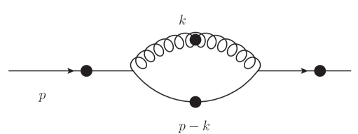
Figure 1: The one-loop diagram contributing to the mass operator in momentum space. Gluon and quark propagators are effective propagators in the presence of an external chromomagnetic field.

The order $\alpha_{s}$ contribution to the ”mass operator” is given by the diagram shown in Fig. 1. The coordinate space $M$ is given then by

$$M(x,x^{\prime})=\phi_{q}(x,x^{\prime})\int\frac{d^{4}p}{(2\pi)^{4}}\exp[ip(x-x^{\prime})]M(p)$$ (10)

where we have used the relation between the external quark charge $q$ and the the charges of the internal quark $q^{\prime}$ and the gluon $Q$: $q=q^{\prime}+Q$ to write

$$\phi_{q}(x,x^{\prime})=\phi_{q^{\prime}}(x,x^{\prime})\phi_{{}_{Q}}(x,x^{\prime})\;.$$

The ”momentum” representation mass operator is

$$M(p)=-g^{2}(T^{A})_{ik}(T^{A})_{ki}\int\frac{d^{4}k}{(2\pi)^{4}}G_{\mu\nu}(k)\gamma^{\mu}S(p-k)\gamma^{\nu}\;.$$ (11)

To get the un-integrated emission probability $P(\omega)$, we use the insertion used in SchwinET :

$$1=\int\limits_{-\infty}^{\infty}d\omega\int\limits_{-\infty}^{\infty}\frac{d\lambda}{2\pi}\exp\{-i\lambda(\omega-k_{o})\}\;.$$

From now on our procedure will follow the steps of SchwinET . To avoid hindering the main result of this paper by technical details we present the main steps and most of the derivation Appendix A.

The exact expression of the one-loop momentum representation $M(p)$, after $k$ and $\lambda$ integration, is

$$M(p)=-2\frac{g^{2}}{(4\pi)^{2}}(T^{A})_{ik}(T^{A})_{ki}\int\limits_{-\infty}^{\infty}d\omega\int\limits_{0}^{\infty}ds\left(\frac{i}{\pi s}\right)^{\frac{1}{2}}$$

$$\int\limits_{0}^{1}\frac{du}{\delta^{\prime}\cos y\cos z}\exp(is\Phi)\left\{me^{iz\Sigma_{3}}+\frac{(1-u)\tan y}{y\delta^{\prime}\cos z}(\vec{\gamma}\cdot\vec{p})_{\perp}\right.$$

$$\left.+\left[m-(p_{o}-\omega)\gamma_{o}+p_{z}(1-u)\gamma_{3}\right]e^{-i(z-2y)\Sigma_{3}}\right\}$$ (12)

Few definitions are made: $y=(1-u)sgQh$; $z=usgq^{\prime}h$

$$\delta^{\prime}=(1-u)\frac{\tan y}{y}+u\frac{\tan z}{z}$$

and the phase factor

$$\Phi=-m^{2}+u(1-u)p_{\parallel}^{2}-u(1-u)\frac{\tan z}{\delta^{\prime}z}\frac{\tan y}{y}+(up_{o}-\omega)^{2}\;.$$

Note that $M(p)$ at this stage is still in a matrix form.

VI Fourier transform: dispersion relation

The expression of $M(p)$ found in the previous section [Eq. (12)] has to be Fourier transformed and then multiplied by the gauge field depending phase $\phi_{q}(x,x^{\prime})$, with the external quark charge $q$, to give $M(x,x^{\prime})$. This can be done using the relations derived by Tsai in Tsai . For instance

$$\phi(x,x^{\prime})\int\frac{d^{4}p}{(2\pi)^{4}}e^{ip(x-x^{\prime})}e^{iA_{o}p_{o}^{2}}e^{iA_{3}p_{3}^{2}}e^{-iBp_{\perp}^{2}}$$

$$=\cos Z\langle x|e^{iA_{o}\Pi_{o}^{2}}e^{iA_{3}\Pi_{3}^{2}}e^{i{\cal S}\Pi_{\perp}^{2}}|x^{\prime}\rangle$$ (13)

The $\Pi$’s are the generalized momentum operators in the presence of a magnetic field. This relation can be easily derived, as shown in Appendix B, if one notices that the right-hand side can be decomposed into three quantum non-relativistic propagators: a free particle of some fictive mass related to $A_{o}$ living in the ”$o$” one-dimensional space, a free particle living in the ”$3$” one dimensional space, and finally a particle living in the transverse plane and under the action of an external magnetic field $H$ perpendicular to the plane. The three propagators are exactly known which give the above relation with $Z=gq{\cal S}$ and

$${\cal S}=\frac{1}{gqh}\tan^{-1}(gqhB)$$

Similar relations are used for the product of exponential factors and $p_{\mu}$ to the left of Eq. (13). The mass operator can then be obtained. This mass operator will be acting on physical quark states satisfying $(\Pi_{\mu}\gamma^{\mu}+m)\psi=0$. Hence it is possible to do the following replacements

$$\hat{\Pi}_{\perp}^{2}\rightarrow\hat{\Pi}_{\parallel}^{2}+gqh\Sigma_{3}-m^{2}\;;\quad\hat{\Pi}_{\parallel}\rightarrow p_{\parallel};,$$

where $p_{\parallel}$ now represents the eigenvalues of $\hat{\Pi}_{\parallel}$ which is not affected by the longitudinal chromomagnetic field.

Applying Tsai’s relations and the external quark equation of motion to Eq. (12) the mass operator will be

$$\hat{M}=-2\frac{g^{2}}{(4\pi)^{2}}(T^{A})_{ik}(T^{A})_{ki}\int d\omega\int ds\left(\frac{i}{\pi s}\right)^{\frac{1}{2}}$$

$$\int du\frac{\cos Z}{\delta^{\prime}\cos y\cos z}\exp(is\Phi^{\prime})\left\{me^{i(z-Z)\Sigma_{3}}\right.$$

$$\left.+\cos Z\frac{(1-u)\tan y}{y\delta^{\prime}\cos z}[(\gamma\cdot p)_{\parallel}-m]\right.$$

$$\left.\!\!\!\!\!\!\!\!+\left[m-(p_{o}-\omega)\gamma_{o}+p_{z}(1-u)\gamma_{3}\right]e^{-i(z+Z-2y)\Sigma_{3}}\right\}$$ (14)

where $Z=gq{\cal S}$, and

$${\cal S}=\frac{1}{gqh}\tan^{-1}\left[su(1-u)\frac{\tan z}{\delta^{\prime}}\frac{\tan y}{y}\right]$$

defined as mentioned before from the Fourier transform. The new phase factor, which is a scalar now, is

$$\Phi^{\prime}=u(p_{o}-\omega)^{2}-(1-u)(up_{3}-\omega^{2})-\frac{\cal S}{s}(p_{o}^{2}-p_{3}^{2}-m^{2})\;.$$ (15)

VII Gamma substitutions

The mass operator has a spinorial/matrix structure. It should be mentioned that we have used the exact dispersion relation for the replacement of $\Pi_{\perp}$ in the phase factor, without solving the equation of motion. However, the Dirac structure in front of the exponential factor in (14) depends on the gamma matrices in a nontrivial way. We use the same approximation done in the literature, which is the weak point of the method: the spinor structure of the incident quark is the same as that of the free particle, i.e., the Dirac spinor $u_{s}(p)$. So sandwiching the mass operator between $u$ and $\bar{u}$, the gamma matrices are replaced by scalar quantities. Simple matrix calculation leads to the following replacement rules: $\gamma_{o}\rightarrow p_{o}/m$, $\gamma_{3}\rightarrow p_{3}/m$, $\Sigma_{3}\rightarrow\eta\frac{1}{m}\left(p_{o}-\frac{p_{z}^{2}}{p_{o}+m}\right)$; $\gamma_{o}\Sigma_{3}\rightarrow\eta(1+\frac{p_{3}^{2}}{m(p_{o}+m)})$; $\gamma_{3}\Sigma_{3}\rightarrow\eta\frac{p_{3}}{m}$.

The $\eta=\pm$ are for the different helicities of the quark. The gamma replacement leads to a scalar mass operator that can be used to obtain $P(\omega)$,

$$M=-2\frac{g^{2}}{(4\pi)^{2}}(T^{A})_{ik}(T^{A})_{ki}\int d\omega\int ds\left(\frac{i}{\pi s}\right)^{\frac{1}{2}}\int du$$

$$\frac{\cos Z}{\delta^{\prime}\cos y\cos z}\exp(is\Phi^{\prime})\left\{m(\cos(z-Z)+\cos(Z+z-2y))\right.$$

$$-i\eta\left(p_{o}-\frac{p_{z}^{2}}{p_{o}+m}\right)(\sin(Z-z)+\sin(Z+z-2y))$$

$$+\cos Z\frac{(1-u)\tan y}{y\delta^{\prime}\cos z}\left(\frac{p_{o}^{2}-p_{3}^{2}-m^{2}}{m}\right)$$

$$-(p_{o}-\omega)\frac{p_{o}}{m}\cos(Z+z-2y)+\frac{p_{z}^{2}}{m}(1-u)\cos(Z+z-2y)$$

$$+i\eta(p_{o}-\omega)\left(1+\frac{p_{3}^{2}}{m(p_{o}+m)}\right)\sin(Z+z-2y)$$

$$\left.-i\eta(1-u)\frac{p_{z}^{2}}{m^{2}}\left(p_{o}-\frac{p_{z}^{2}}{p_{o}+m}\right)\sin(Z+z-2y)\right\}$$ (16)

Note that this expression has helicity information that can be explored in a way similar to Tuchin .

VII.1 The Abelian limit

The results found in SchwinET can be easily obtained from our expression in Eq. (16). The non-Abelian character can be waived if we set the gluon charge $Q$ to zero hence $y=0$; remove the color factor $T^{A}T^{A}$ in $M$; and consider the motion of the incident quark in the transverse plane, i.e., take $p_{3}=0$. Besides, we have to set the index of refraction $n=1$ in SchwinET ; hence the parameters $\delta$, $E$, $\widetilde{\beta}$, $\delta^{\prime}$ of SchwinET will be in our notation (for $y=0=p_{3}$) $\delta=1$, $E\rightarrow p_{o}$, $\delta^{\prime}\rightarrow\delta^{\prime}$, $\widetilde{\beta}\rightarrow Z$.

The above simplifications lead to

$$M_{abelian}=2\frac{g^{2}}{(4\pi)^{2}}\int d\omega\int ds\left(\frac{i}{\pi s}\right)^{\frac{1}{2}}\int du\exp(is\Phi^{\prime})\frac{m}{\Delta^{1/2}}$$

$$\left\{\cos(Z-z)\right.-i\eta\frac{p_{o}}{m}\sin(Z-z)$$

$$+\frac{\omega}{m}\frac{p_{o}}{m}\cos(Z+z)-i\eta\frac{\omega}{m}\sin(Z+z)$$

$$\left.+\frac{p_{o}^{2}-m^{2}}{m^{2}}\left[\frac{1-u}{\Delta^{1/2}}-\cos(Z+z)\right]\!\!\right\}$$ (17)

whereas in SchwinET $\Delta^{1/2}=(\delta^{\prime}\cos z)/\cos Z$. Eq. (17) coincides with equation (3.39 a) of SchwinET .

VII.2 Small $s$ limit

By analyzing Eq. (16) it is clear that the $s$-integration is dominated by small a $s$ region. The small $s$ expansion of the phase factor $\Phi^{\prime}$ gives

$$\Phi^{\prime}\approx(up_{o}-\omega)^{2}-m^{2}u^{2}$$

$$-\left[gq^{\prime}uh-gQh(1-u)\right]^{2}\frac{s^{2}}{3}\left[u^{2}(1-u)^{2}(p_{o}^{2}-p_{3}^{2})-m^{2}\right]$$ (18)

The $u$-integration can then be approximated by a Gaussian integration:

$$\int_{0}^{1}duf(u)e^{is(up_{o}-u)^{2}}\approx f(u\approx\frac{\omega}{p_{o}})\frac{1}{2ip_{o}}\sqrt{\frac{\pi}{is}}$$ (19)

In this approximation the variable $u$ is replaced by the gluon energy fraction $x=\omega/p_{o}$. After the $u$-integration the phase factor will be

$$s\Phi^{\prime}\rightarrow-m^{2}sx^{2}-\frac{\mathbf{f}^{2}}{3}s^{3}\left[x^{2}(1-x)^{2}(p_{o}^{2}-p_{3}^{2})-m^{2}\right]$$ (20)

where we have defined the vector

$$\mathbf{f}=gq^{\prime}x\mathbf{H}-gQ(1-x)\mathbf{H}$$

which represents a fictive magnetic force on an intermediate gluon-quark system.

VII.3 Zakharov method

Before proceeding to an explicit comparison of our result with the one found in Zak1 ; we present Zakharov’s method in its simplest ”display.”

Consider first a fast scalar particle whose first quantized wave function satisfying the Klein-Gordon equation

$$(\frac{\partial^{2}}{\partial t^{2}}-\frac{\partial^{2}}{\partial\mathbf{r}^{2}})\psi=m^{2}\psi\;.$$ (21)

For a fast particle moving along the $z$-axis with large energy $E$, the wave function can be written as

$$\psi(t,\mathbf{r})=\exp\left(-iE\xi\right)\phi(z,\xi,\mathbf{\rho})$$ (22)

where $\xi=t-z$, $\mathbf{r}=(z,\mathbf{\rho})$. For fixed $\xi$ the ”transverse” wave function $\phi$ satisfies the equation

$$i\frac{\partial\phi}{\partial z}=\left(\frac{\mathbf{p}_{\perp}^{2}+m^{2}}{2E}\right)\phi+\frac{\partial^{2}\phi}{\partial z^{2}}$$ (23)

Besides, in the low mass limit or for $m\ll E$ the above equation simplifies to

$$i\frac{\partial\phi}{\partial z}=\left(\frac{\mathbf{p}_{\perp}^{2}+m^{2}}{2E}\right)\phi\;.$$ (24)

Which is a two-dimensional Schrödinger equation with a mass $E$. The solution to the above equation can be easily obtained,

$$\phi_{p_{z},p_{\perp}}(z,{\bf\rho})=e^{i{\mathbf{p}_{\perp}}\cdot{\bf\rho}}e^{-i\int\limits_{0}^{z}\left(\frac{\mathbf{p}_{\perp}^{2}+m^{2}}{2p_{z}}\right)dz}\;,$$ (25)

which can be interpreted as a plane wave. The $\xi$ dependence emerges only via boundary conditions for the transverse wave function. So we have an evolution equation along each line $\xi={\rm const}$.

If we consider now a parton of color charge $Q$ in an external field $H$, represented by a gauge field $A_{\mu}$, the equation of motion becomes

$$i\frac{\partial\phi}{\partial z}=\left\{\frac{(\mathbf{p}-gQ\mathbf{A})_{\perp}^{2}+m^{2}}{2E}+gQ(A^{o}-A^{3})\right\}\phi\;.$$ (26)

The field configuration considered in Zak1 is such that $\vec{A}=0=A^{o}$ and $A_{3}=[\mathbf{H}\times\mathbf{\rho}]_{3}$; hence the magnetic field is taken to be in the transverse plane. The wave function is then simply found to be

$$\phi_{p_{z},p_{\perp}}(z,{\bf\rho})=e^{i{\vec{p}_{\perp}}\cdot{\bf\rho}}e^{-i\int\limits_{0}^{z}\left(\frac{\mathbf{p}_{\perp}^{2}+m^{2}}{2p_{z}}\right)dz}\;,$$ (27)

But now the transverse momentum is a solution of the ”classical equation of motion”

$$\frac{d\mathbf{p}_{\perp}}{dz}=\mathbf{F}\;.$$

This is applied to the incident quark as well as to the outgoing gluon and quark .

The final result of Zak1 can be written as

$$\frac{dP}{dLdx}=\frac{i\mu}{2\pi}\int\limits_{\infty}^{-\infty}\frac{d\tau}{\tau}\left[\frac{g_{1}}{\mu^{2}}\left(\epsilon^{2}+\frac{\mathbf{f^{2}\tau^{2}}}{2}\right)-g_{2}\right]$$

$$\exp\left\{-i\left[\frac{\epsilon^{2}\tau}{2\mu}+\frac{\mathbf{f}^{2}\tau^{3}}{24\mu}\right]\right\}$$ (28)

where $\mu=Ex(1-x)$ (an effective mass), $g_{1}=C\alpha_{s}(1-x+x^{2})/x$ (non-spin-flip vertex factor), $g_{2}=C\alpha_{s}m_{q}^{2}x^{3}/2\mu^{2}$ (spin-flip vertex factor), $\epsilon=m_{q}^{2}x^{2}+m_{g}^{2}(1-x)^{2}$, and as in our approach the fictive force of a quark-gluon system is $\mathbf{f}=x\mathbf{F}_{q^{\prime}}-(1-x)\mathbf{F}_{g}$.

Comparing a particle propagation in a longitudinal field to that of a transverse field configuration is not intuitive. However, in an infinite (nonrealistic) medium, and for a static (non-propagating) magnetic field, and with a vanishing electric field, it is the propagation direction of the incident parton which gives the meaning of the longitudinal/transverse directions. So if in our approach we take $p_{z}=0$ we will be the closest to the configuration of Zak1 , where the transverse direction is mapped into the longitudinal direction in the following ways:

• Present configuration: a particle moving in the transverse plane under the action of a longitudinal field.

• Zakharov’s configuration: a fast particle moving along the longitudinal direction and a transverse magnetic field.

It is closest but not the same, since in Zak1 , transverse momenta are not set to zero.

So setting $p_{z}=0$, $p_{o}=E$ and $s=\tau/(2\mu)$ in Eq. (20) we obtain the same phase given in Eq. (28) for a zero gluon mass. However, not surprisingly, the prefactor of our approximated expression does not match that of Eq. (28).

VII.4 Shuryak et al

It is now clear that our agreement with Zak1 leads to the conclusion that the results of ShuryaZ are ”defective”. As the author of ShuryaZ did not give enough details about their approximation method it is hard to trace the exact source of inconsistency in ShuryaZ . However we expect that their asymmetric treatment of the quark and gluon propagators leads to a nonsystematic approximation/expansion. For instance, the important Bohm-Aharonov phase, which plays an important role in our derivation, was absorbed in an unjustified way. Consequently the fictive force $\mathbf{f}$ was badly approximated.

VIII Conclusions

The generalization of QED synchrotron radiation to the QCD case was done with the minimal possible complications. It is shown that the QED case can be obtained as a special limit. The comparison with the path integral approach of Zakharov has shown consistent results. This will hopefully ”solve” the debate about gluon synchrotron radiation.

It is possible now to extend our method to include nonzero gluon mass (thermal mass) and combinations of longitudinal and transverse chromoelectric and chromomagnetic fields with an arbitrary color index. This is under current investigation.

Appendix A Schwinger et al procedure

Our derivation follows the recipe of SchwinET . We present in what follows the main steps needed to get equation (12).

The first step to follow is the change of variables: $s_{1}=(1-u)s$, $s_{2}=us$, where $0\leq u\leq 1$, and $s$ is positive. The $\lambda$ and $k$ integration is based on Gaussian integration and saddle point approximation. Hence the exponential factor is factored out in the expression of $M$; this can be written as

$$M(p)=\int\limits_{0}^{1}du\int d^{4}k\int\limits_{-\infty}^{\infty}d\lambda d\omega\int\limits_{0}^{\infty}dsM_{{}_{\rm Dirac}}\exp\left(is(\chi-\frac{\lambda\omega}{s})\right)$$ (29)

where $M_{{}_{\rm Dirac}}$ contains the Dirac structure of the self-energy diagram and all the non-exponential terms. The function $\chi$ can be split into a momentum dependent part $\chi_{1}$ and a $\lambda$ dependent function $\chi_{o}$, $\chi=\chi_{o}+\chi_{1}$, such that

$$\chi_{1}=\left(k_{o}-(up_{o}-\frac{\lambda}{2s})\right)^{2}-(k_{3}-up_{3})^{2}-\delta^{\prime}\left(\vec{k}_{\perp}-\frac{u\tan z}{z\delta^{\prime}}\vec{p}_{\perp}\right)^{2}$$

while

$$\chi_{o}=-\frac{1}{s^{2}}\left(\frac{\lambda^{2}}{4}-up_{o}\lambda s\right)+\Phi$$

where $\delta^{\prime}$ and $\Phi$ are as defined before.

We perform now the $k$ integration using the Gaussian form(s)

$$\int\frac{d^{4}k}{(2\pi)^{4}}\exp(is\chi_{1})\left[1,k_{o},k_{3},\vec{k}_{\perp}\right]=$$

$$\frac{i}{\delta^{\prime}(4\pi)^{2}s^{2}}\left[1,up_{o}-\frac{\lambda}{2s},up_{3},\frac{u\tan z}{\delta^{\prime}z}\vec{p}_{\perp}\right]$$ (30)

For the $\lambda$ integration

$$\int\frac{d\lambda}{2\pi}\exp(is\chi_{o}-i\lambda\omega)[1,\lambda]=$$

$$\left(\frac{s}{i\pi}\right)^{1/2}e^{is(\Phi+(up_{o}-\omega)^{2})}[1,2s(up_{o}-\omega)]$$ (31)

The remaining, lengthy but straightforward, step needed to get equation (12) is the Dirac structure simplification/contractions.

Appendix B Tsai transformation to coordinate space

We give a simple derivation for equation (13) which is different from the initial method of Tsai Tsai .

Consider a non-relativistic particle of mass $m$ and charge $g$ in a uniform magnetic field $H$. The general expression of the non-relativistic propagator in coordinate space is

$$K(\vec{r},\tau,\vec{r}_{o},0)=\langle\vec{r}|\exp\left(-i{\cal H}\frac{\tau}{\hbar}\right)|\vec{r}_{o}\rangle$$

$$=\left(\frac{m}{2i\pi\hbar s}\right)^{3/2}\frac{gH\tau/2m}{\sin(gH\tau)/2m}\exp\left(\frac{iS_{\rm cl}}{\hbar}\right)$$ (32)

where ${\cal H}$ is the particle Hamiltonian

$${\cal H}=\frac{\Pi_{\perp}^{2}}{2m}-\frac{\Pi_{\parallel}^{2}}{2m}$$

with $\Pi$ the generalized momentum. The classical action $S_{\rm cl}$ in the presence of a magnetic field is

$$S_{\rm cl}=\frac{gH}{2}\{\frac{1}{2}\left[(x-x_{o})^{2}+(y-y_{o})^{2}\right]\cot(gH\tau/2m)$$

$$+(x_{o}y-y_{o}x)\}+\frac{m}{2\tau}(z-z_{o})^{2}$$ (33)

The non-translational invariant term $(x_{o}y-y_{o}x)$ in the action gives the Bohm-Aharonov phase, if we assume a straight line trajectory. Hence the four-dimensional generalization will be

$$K(x^{\mu},\tau,x^{\prime\mu},0)=\Phi(x,x^{\prime})\left(\frac{1}{4\pi\tau}\right)^{2}\frac{z}{\sin z}$$

$$\exp\left(igH\cot z\frac{(\vec{x}_{\perp}-\vec{x}^{\prime}_{\perp})^{2}}{4}\right)\exp\left(-i\frac{(x_{\parallel}-x_{\parallel}^{\prime})^{2}}{4\tau}\right)$$ (34)

where $z=gH\tau$. It is now possible to write the propagator $K$ in momentum space. We use the Fourier transform

$$\frac{z\pi}{i\tau\sin z}\exp\left(igH\cot z\frac{(\vec{x}_{\perp}-\vec{x}^{\prime}_{\perp})^{2}}{4}\right)=$$

$$\int\frac{d^{2}p_{\perp}}{\cos z}\exp\left(-i\vec{p}_{\perp}\cdot(\vec{x}_{\perp}-\vec{x}_{\perp}^{\prime})\right)\exp\left(-i\tau\frac{\tan z}{z}p_{\perp}^{2}\right)$$ (35)

This is similarly done for the longitudinal part ($\parallel$) of the propagator. Hence

$$K(x^{\mu},\tau,x^{\prime\mu},0)=\langle x|\exp\left(i\tau\Pi^{2}\right)|x^{\prime}\rangle$$

$$=\Phi(x,x^{\prime})\int\frac{d^{4}P}{(2\pi)^{4}}e^{iP\cdot(x-x^{\prime})}\frac{e^{i\tau p_{\parallel}^{2}}}{\cos z}e^{-i\tau\frac{\tan z}{z}p_{\perp}^{2}}$$ (36)

where we have set $m=1/2$ and $\hbar=1$ in the nonrelativistic formula. This Formula is the same as equation (13) with appropriate relabeling of field and time parameters.

References

- [1] R. J. Friesa, J. I. Kapustaa, Yang Lia, Nucl. Phys. A 774, 861 (2006).
- [2] T. Lappi, L. McLerran, Nucl. Phys. A 772, 200 (2006).
- [3] I. M. Dremin J. Phys. G: Nucl. Part. Phys. 34, S831 (2007).
- [4] E. V. Shuryak and I. Zahed, Phys. Rev. D 67, 054025 (2003).
- [5] B.G. Zakharov, JETP Letters 88, 475 (2008).
- [6] K. Tuchin, Phys. Rev. C 82, 034904 (2010), Phys. Rev. C 83, 039903 (2011).
- [7] A. A. Sokolov, N.P. Klepikov, I.M. Ternov, Zh. Eksp. Teor. Fiz. 24, 249(1953).
- [8] J. Schwinger, Proc. Nat. Acad. Sci. 40, 132 (1954).
- [9] J. Schwinger, W. Tsai, T. Erber, Annals of physics 96, 303 (1976).
- [10] W. Tsai, Phys. Rev. D 10, 1342 (1974).