Renewal-Theoretical Dynamic Spectrum Access in Cognitive Radio Networks with Unknown Primary Behavior

Abstract

Dynamic spectrum access in cognitive radio networks can greatly improve the spectrum utilization efficiency. Nevertheless, interference may be introduced to the Primary User (PU) when the Secondary Users (SUs) dynamically utilize the PU’s licensed channels. If the SUs can be synchronous with the PU’s time slots, the interference is mainly due to their imperfect spectrum sensing of the primary channel. However, if the SUs have no knowledge about the PU’s exact communication mechanism, additional interference may occur. In this paper, we propose a dynamic spectrum access protocol for the SUs confronting with unknown primary behavior and study the interference caused by their dynamic access. Through analyzing the SUs’ dynamic behavior in the primary channel which is modeled as an ON-OFF process, we prove that the SUs’ communication behavior is a renewal process. Based on the Renewal Theory, we quantify the interference caused by the SUs and derive the corresponding close-form expressions. With the interference analysis, we study how to optimize the SUs’ performance under the constraints of the PU’s communication quality of service (QoS) and the secondary network’s stability. Finally, simulation results are shown to verify the effectiveness of our analysis.

I Introduction

Cognitive radio is considered as an effective approach to mitigate the problem of crowded electromagnetic radio spectrums. Compared with static spectrum allocation, dynamic spectrum access (DSA) technology can greatly enhance the utilization efficiency of the existing spectrum resources [1]. In DSA, devices with cognitive capability can dynamically access the licensed spectrum in an opportunistic way, under the condition that the interference to the communication activities in the licensed spectrum is minimized [2]. Such cognitive devices are called as Secondary Users (SUs), while the licensed users as Primary Users (PUs) and the available spectrum resource for the SUs is referred to as “spectrum hole”.

One of the most important issues in the DSA technology is to control the SUs’ adverse interference to the normal communication activities of the PU in licensed bands [3]. One way is to strictly prevent the SUs from interfering the PU in both time domain and frequency domain [4], and the other approach is to allow interference but minimizing the interference effect to the PU . For the latter approach, the key problem is to model and analyze the interference caused by the SUs to reveal the quantitative impacts on the PU. Most of the existing works on interference modeling can be categorized into two classes: spatial interference model and accumulated interference model. The spatial interference model is to study how the interference caused by the SUs varies with their spatial positions [6][7][8], while the accumulated interference model focuses on analyzing the accumulated interference power of the SUs at primary receiver through adopting different channel fading models such as what discussed in [9][10] with exponential path loss, and in [11][12][13] with both exponential path loss and log-normal shadowing. Moreover, in [14][15][16][17], the SUs are modeled as separate queuing systems, where the interference and interactions among these queues are analyzed to satisfy the stability region.

However, most traditional interference analysis approaches are based on aggregating the SUs’ transmission power with different path fading coefficients, regardless the communication behaviors of the PU and the SUs. In this paper, we will study the interference through analyzing the relationship between the SUs’ dynamic access and the states of the primary channel in the MAC layer. Especially, we will focus on the situation when the SUs are confronted with unknown primary behavior. If the SUs have the perfect knowledge of the PU’s communication mechanism, the interference is mainly from the imperfect sensing which has been well studied [18]. To simplify the analysis and give more insights into the interference analysis, we assumed perfect spectrum sensing in this paper. We show that the SUs’ dynamic behavior in the primary channel is a renewal process and quantify the corresponding interference caused by the SUs’ behavior based on the Renewal Theory [19]. There are some works using renewal theory for cognitive radio networks. In [20], the primary channel was modeled as an ON-OFF renewal process to study how to efficiently discover spectrum holes through dynamically adjusting the SUs’ sensing period. As the extension works of [20], Xue et. al. designed a periodical MAC protocol for the SUs in [21], while Tang and Chew analyzed the periodical sensing errors in [22]. In [23][24], the authors discussed how to efficiently perform channel access and switch according to the residual time of the ON-OFF process in the primary channel. Based on the assumption that the primary channel is an ON-OFF renewal process, the delay performance of the SUs were analyzed in [25][26]. However, all these related works have only modeled the PU’s behavior in the primary channel as an ON-OFF process. In this paper, we further show and study the renewal characteristic of the SUs’ communication behavior and analyze the interference to the PU when they dynamically access the primary channel.

The main contributions of this paper are summarized as follows.

1. We propose a dynamic spectrum access protocol for the SUs under the scenario that they have no knowledge about the PU’s exact communication mechanism. By treating the SUs as customers and the primary channel as the server, our system can be regarded as a queuing system.

2. Different from the traditional interference analysis which calculates the SUs’ aggregated signal power at the primary receiver in the physical layer, we introduce a new way to quantify the interference caused by the SUs in the MAC layer. This interference quantity represents the proportion of the periods when the PUs’ communication are interfered by the SUs’ dynamic access.

3. We prove that the SUs’ communication behavior in the primary channel is a renewal process and derive the close-form expressions for the interference quantity using the Renewal Theory.

4. To guarantee the PUs’ communication quality of service (QoS) and maintain the stability of the secondary network, we formulate the problem of controlling the SUs’ dynamic access as an optimization problem, where the objective function is to maximize the SUs’ average data rate with two constraints: the PU’s average data rate should not be lower than a pre-determined threshold and the SUs’ arrival interval and transmission time should satisfy the stability condition.

The rest of this paper is organized as follows. Firstly, our system model is described in Section II. Then, we present the proposed dynamic spectrum access protocol for the SUs in Section III. We derive the close-form expressions for the interference quantity of two different scenarios in Section IV and V respectively. In Section VI, we discuss how to optimize the SUs’ communication performance according to the interference analysis. Finally, simulation results are shown in Section VII and conclusion is drawn in Section VIII.

II System Model

II-A Network Entity

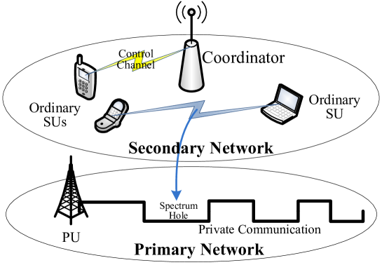
Figure 1: Network entity.

As shown in Fig. 1, we consider a cognitive radio network with one PU and $M$ SUs operating on one primary channel. The PU has priority to occupy the channel at any time, while the SUs are allowed to temporarily access the channel under the condition that the PU’s communication QoS is guaranteed. An important feature of our system is that the communication mechanism in the primary network is private, i.e., the SUs have no knowledge when the PU’s communication will arrive.

For the secondary network, $M$ SUs form a group under the management of one coordinator. The coordinator is in charge of observing the PU’s behavior, deciding the availability of the primary channel, coordinating and controlling the SUs’ dynamic access. There is a control channel for command exchange between the ordinary SUs and the coordinator. The SUs need to opportunistically access the primary channel to acquire more bandwidth for high data rate transmission, e.g., multimedia transmission. Considering that the ordinary SUs are usually small-size and power-limit mobile terminals, spectrum sensing is only performed by the coordinator. Meanwhile, we assume that all the ordinary SUs are half-duplex, which means that they cannot simultaneously transmit and receive data packet.

II-B Primary Channel State Model

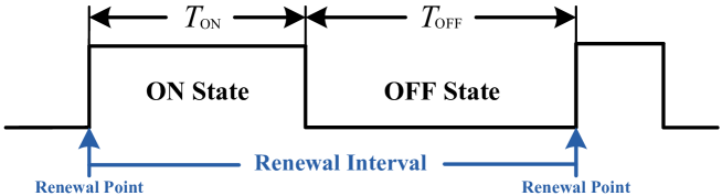
Figure 2: Illustration of the ON-OFF primary channel state.

Since the SUs have no idea about the exact communication mechanism of the primary network and hence cannot be synchronous with the PU, there is no concept of “time slot” in the primary channel from the SUs’ points of view. Instead, the primary channel just alternatively switches between ON state and OFF state, as shown in Fig. 2. The ON state means the channel is being occupied by the PU, while the OFF state is the “spectrum hole” which can be freely occupied by the SUs.

We model the length of the ON state and OFF state by two random variables $T_{\mbox{\tiny{ON}}}$ and $T_{\mbox{\tiny{OFF}}}$ respectively. According to different types of the primary services (e.g., digital TV broadcasting or cellular communication), $T_{\mbox{\tiny{ON}}}$ and $T_{\mbox{\tiny{OFF}}}$ statistically satisfy different distributions. In this paper, we assume that $T_{\mbox{\tiny{ON}}}$ and $T_{\mbox{\tiny{OFF}}}$ are independent and satisfy exponential distributions with parameter $\lambda_{1}$ and $\lambda_{0}$ respectively, denoted by $f_{\mbox{\tiny{ON}}}(t)$ and $f_{\mbox{\tiny{OFF}}}(t)$ as follows

$$\left\{\begin{array}[]{l}T_{\mbox{\tiny{ON} }}\sim f_{\mbox{\tiny{ON }}}(t)=\frac{1}{\lambda_{1}}e^{-t/\lambda_{1}},\vspace{2mm}\\ T_{\mbox{\tiny{OFF}}}\sim f_{\mbox{\tiny{OFF}}}(t)=\frac{1}{\lambda_{0}}e^{-t/\lambda_{0}}.\end{array}\right.$$ (1)

In such a case, the expected lengths of the ON state and OFF state are $\lambda_{1}$ and $\lambda_{0}$ accordingly. These two important parameters $\lambda_{1}$ and $\lambda_{0}$ can be effectively estimated by a maximum likelihood estimator [20]. Such an ON-OFF behavior of the PU is a combination of two Poisson process, which is a renewal process [19]. The renewal interval is $T_{p}=T_{\mbox{\tiny{ON}}}+T_{\mbox{\tiny{OFF}}}$ and the distribution of $T_{p}$, denoted by $f_{p}(t)$, is

$$f_{p}(t)=f_{\mbox{\tiny{ON}}}(t)\ast f_{\mbox{\tiny{OFF}}}(t),$$ (2)

where the symbol “$\ast$” represents the convolution operation.

III Secondary Users’ Dynamic Spectrum Access Protocol

In this section, we will design and analyze the SUs’ communication behavior including how the SUs dynamically access the primary channel and how the coordinator manages the group of SUs. Based on the behavior analysis, we can further study the interference caused by the SUs’ access.

III-A Dynamic Spectrum Access Protocol

In our protocol, the SUs who want to transmit data must first inform the coordinator with a request command, which can also be listened by the corresponding receiver. The coordinator sequentially responds to the requesting SUs by a confirmation command according to the First-In-First-Out (FIFO) rule. The SU who has received the confirmation should immediately transmit data with time $T_{t}$ over the primary channel. During the whole process, all the spectrum sensing and channel estimation works are done by the coordinator simultaneously. The proposed dynamic access protocol for both ordinary SUs and the coordinator is summarized in Algorithm 1. Considering the existence of malicious SUs who may keep requesting for packet transmission, we restrict each SU’s overall times of requesting within a constant period of time. Once the coordinator discovered that one SU’s requesting frequency exceeds the pre-determined threshold, it will reject this SU’s request within a punishing period.

III-B Queuing Model

According to the proposed access protocol, the secondary network can be modeled as a queueing system as shown in Fig. 3. We assume that the requests from all SUs arrive by a Poisson process at the coordinator with rate $\lambda_{s}^{-1}$. In such a case, the arrival intervals of SUs’ requests at the coordinator, denoted by $T_{s}$, satisfies the exponential distribution with expectation $\lambda_{s}$, i.e., $T_{s}\sim f_{s}(t)=\frac{1}{\lambda_{s}}e^{-t/\lambda_{s}}$.

In this queuing system, the coordinator’s buffer only records the sequence of the SUs’ request, instead of the specific data packets. The packets are stored in each SU’s own data memory, which is considered as infinite length. In such a case, we can also regard the buffer in the coordinator as infinite length. For the service time of each SU, it is the sum of the transmission time $T_{t}$ and the waiting time if $T_{t}$ ends in the ON state as show in Fig. 3. In our model, the time consumed by command exchange between ordinary SUs and the coordinator is not taken into account, since it is negligible compared to $T_{t}$, $\lambda_{0}$ and $\lambda_{1}$. Based on this queuing model, we can analyze the interference caused by the SUs’ dynamic access.

Algorithm 1 SUs’ Dynamic Spectrum Access Protocol.

I. For the ordinary SU

1:  if A SU has one packet to transmit then

2:     • Send a request command to the coordinator through the secondary control channel

3:     while No confirmation from the coordinator do

4:        • Store the packet in its memory and wait

5:     end while

6:     • Transmit its packet after confirmation

7:  end if

II. For the coordinator

1:  • Estimate the primary channel’s parameters $\lambda_{0}$ and $\lambda_{1}$

2:  if A request command is received then

3:     • Register the SU’s request on the waiting list according to the FIFO rule

4:  end if

5:  while The primary channel is in the OFF state do

6:     • Response to the requesting SU on the top of the waiting list with a confirmation command

7:     • Wait for transmission time $T_{t}$

8:  end while

9:  • Keep sensing the primary channel

III-C Interference Quantity

If the SUs have the perfect knowledge of communication scheme in the primary network, e.g. the primary channel is slotted and all SUs can be synchronous with the PU, then the SUs can immediately vacate the occupied channel by the end of the slot. In such a case, the potential interference only comes from the SUs’ imperfect spectrum sensing. However, when an SU is confronted with unknown primary behavior, additional interference will appear since the SU may fail to discover the PU’s recurrence when it is transmitting packet in the primary channel, as shown by the shaded regions in Fig. 3. The essential reason is that the half-duplex SUs cannot receive any command from the coordinator during data transmission or receiving. Therefore, the interference under such a scenario is mainly due to the SUs’ failure of discovering the PU’s recurrence during their access time.

In most of the existing works -[17], interference to the PU was usually measured as the quantity of SUs’ signal power at primary receiver in the physical layer. In this paper, we will measure the interference quantity based on communication behaviors of the PU and SUs in the MAC layer. The shaded regions in Fig. 3 indicate the interference periods in the ON state of the primary channel. In order to illustrate the impacts of these interference periods on the PU, we define the interference quantity $Q_{I}$ as follows.

Definition 1: The interference quantity $Q_{I}$ is the proportion of accumulated interference periods to the length of all ON states in the primary channel within a long period time, which can be written by

$$Q_{I}=\lim\limits_{T\rightarrow+\infty}\frac{\sum\limits_{T}\mbox{Interference periods}}{\sum\limits_{T}T_{\mbox{\tiny{ON}}}}.$$ (3)

In the following sections, we will derive the close form of $Q_{I}$ in two different scenarios listed below.

• $Q_{I_{1}}$: SUs with arrival interval $\lambda_{s}=0$.

• $Q_{I_{2}}$: SUs with constant arrival interval $\lambda_{s}\neq 0$.

IV Interference Caused by SUs with Zero Arrival Interval

In this section, we will discuss the interference to the PU when the average arrival interval of all SUs’ requests $\lambda_{s}=0$, i.e., the arrival rate $\lambda_{s}^{-1}=+\infty$. In the practical scenario, $\lambda_{s}^{-1}=+\infty$ is corresponding to the situation when each SU has plenty of packets to transmit, resulting in an extremely high arrival rate of all SUs’ requests at the coordinator, i.e., $\lambda_{s}^{-1}\rightarrow+\infty$. In such a case, the coordinator’s buffer is non-empty all the time, which means the SUs always want to transmit packets in the primary channel. Such a scenario is the worst case for the PU since the maximum interference from the SUs is considered.

IV-A SUs’ Communication Behavior Analysis

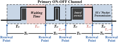
(a) SUs’ renewal process.

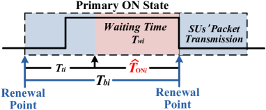
(b) SUs’ waiting time $T_{w}$.

Figure 4: Illustration of the SUs’ behavior in the primary channel when $\lambda_{s}=0$.

Since $\lambda_{s}=0$ means the coordinator always has requests in its buffer, the SUs are either transmitting one packet or waiting for the OFF state. As shown in Fig. 4-(a), the SUs’ behavior dynamically switches between transmitting one packet and waiting for the OFF state. The waiting time, denoted by $T_{w}$, will appear if the previous transmission ends in the ON state, and the value of $T_{w}$ is determined by the length of the remaining time in the primary channel’s ON state. As we discussed in Section III-C, the interference to the PU only occurs during the SUs’ transmission time $T_{t}$. Therefore, the interference quantity is determined by the occurrence probability of $T_{t}$. In the following, we will analyze the SUs’ communication behavior based on Renewal Theory.

Theorem 1: When the SUs’ transmission requests arrive by Poisson process with average arrival interval $\lambda_{s}=0$, the SUs’ communication behavior is a renewal process in the primary channel.

Proof:

As shown in Fig. 4-(a), we use $T_{b}$ to denote the interval of two adjacent transmission beginnings, i.e., $T_{b}=T_{t}+T_{w}$. According to the Renewal Theory [19], the SUs’ communication behavior is a renewal process if and only if $T_{b1}$, $T_{b2}$, …is a sequence of positive independent identically distributed (i.i.d) random variables. Since the packet transmission time $T_{t}$ is a fixed constant, Theorem 1 will hold as long as we can prove that all $T_{w1}$, $T_{w2}$ …are i.i.d.

On one hand, if $T_{ti}$ ends in the OFF state, the following waiting time $T_{wi}$ will be 0, such as $T_{w2}$ and $T_{w4}$ in Fig. 4-(a). On the other hand, if $T_{ti}$ ends in the ON state, the length of $T_{wi}$ will depend on when this ON state terminates, which can be specifically illustrated in Fig. 4-(b). In the second case, according to the Renewal Theory [19], $T_{w}$ is equivalent to the forward recurrence time of the ON state, $\widehat{T}_{\mbox{\tiny{ON}}}$, the distribution of which is only related to that of the ON state. Thus, we can summarize $T_{wi}$ as follows

$$T_{wi}=\left\{\begin{array}[]{l}0_{\quad}\quad\ \ \ \ \ T_{ti}\mbox{\emph{ ends in the OFF state},}\vspace{2mm}\\ \widehat{T}_{\mbox{\tiny{ONi}}}\quad\ \ \ \ \ T_{ti}\mbox{\emph{ ends in the ON state}}.\end{array}\right.\$$ (4)

From (4), it can be seen that all $T_{wi}$s are identically distributed. Meanwhile, since each $T_{wi}$ is only determined by the corresponding $T_{ti}$ and $\widehat{T}_{\mbox{\tiny{ONi}}}$, all $T_{wi}$s are independent with each other. Thus, the sequence of the waiting time $T_{w1}$, $T_{w2}$ …are i.i.d, which means all $T_{b1}$, $T_{b2}$ …are also i.i.d. Therefore, the SUs’ communication behavior is a renewal process. ∎

IV-B Interference Quantity Analysis

In order to analyze the interference during the SUs’ one packet transmission time $T_{t}$, we first introduce a new function, $I(t)$, defined as follows.

Definition 2: $I(t)$ is the expected accumulated interference to the PU within a period of time $t$, where $t$ has two special characteristics listed as follows

• period $t$ always begins at the OFF state of the primary channel,

• during $t$, the SUs keep transmitting packets in the primary channel.

According to Definition 1, Definition 2 and Theorem 1, the interference quantity $Q_{I_{1}}$ (when $\lambda_{s}=0$) can be calculated by

$$Q_{I_{1}}=\frac{I(T_{t})}{I(T_{t})+\mathbb{E}(T_{w})},$$ (5)

where $I(T_{t})$ is the expected interference generated during the SUs’ transmission time $T_{t}$, $\mathbb{E}(T_{w})$ is the expectation of SUs’ waiting time $T_{w}$, during which the primary channel is always in the ON state and no interference from the SUs occurs. In the following, we will derive the close-form expressions for $I(T_{t})$ and $\mathbb{E}(T_{w})$ respectively.

IV-B1 Expected interference $I(T_{t})$

According to Definition 2, $I(t)$ is the expected length of all ON states within a period of time $t$, given that $t$ begins at the OFF state. According to the Renewal Theory [19], the PU’s ON-OFF behavior is a renewal process. Therefore, we can derive $I(t)$ through solving the renewal equation (6) according to the following Theorem 2.

Theorem 2: $I(t)$ satisfies the renewal equation as follows

$$I(t)=\lambda_{1}F_{p}(t)+\int_{0}^{t}I(t-w)f_{p}(w)dw,$$ (6)

where $f_{p}(t)$ is the p.d.f of the PU’s renewal interval given in (2) and $F_{p}(t)$ is the corresponding cumulative distribution function (c.d.f).

Proof:

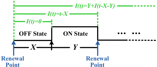
Figure 5: Illustration of function $I(t)$.

Let $X$ denote the first OFF state and $Y$ denote the first ON state, as shown in Fig. 5. Thus, we can write the recursive expression of function $I(t)$ as follows

$$I(t)=\left\{\begin{array}[]{ll}0&t\leq X,\vspace{2mm}\\ t-X&X\leq t\leq X+Y,\vspace{2mm}\\ Y+I(t-X-Y)&X+Y\leq t,\end{array}\right.$$ (7)

where $X\sim f_{\mbox{\tiny{OFF}}}(x)=\frac{1}{\lambda_{0}}e^{-x/\lambda_{0}}\vspace{2mm}$ and $Y\sim f_{\mbox{\tiny{ON}}}(y)=\frac{1}{\lambda_{1}}e^{-y/\lambda_{1}}.$

Since $X$ and $Y$ are independent, their joint distribution $f_{XY}(x,y)=f_{\mbox{\tiny{OFF}}}(x)f_{\mbox{\tiny{ON}}}(y)$. In such a case, $I(t)$ can be re-written as follows

$$I(t)\!\!\!\! = \!\!\!\!\!\!\iint\limits_{x\leq t\leq x+y}(t-x)f_{XY}(x,y)dxdy+\iint\limits_{x+y\leq t}\big{[}y+I(t-x-y)\big{]}f_{XY}(x,y)dxdy,\quad\quad\quad\quad\quad\quad\quad\quad$$ (8)

$$= \!\!\!\!\int_{0}^{t}(t-x)f_{\mbox{\tiny{OFF}}}(x)dx\!+\!\!\iint\limits_{x+y\leq t}I(t-x-y)f_{\mbox{\tiny{OFF}}}(x)f_{\mbox{\tiny{ON}}}(y)dxdy-\!\!\!\iint\limits_{x+y\leq t}(t-x-y)f_{\mbox{\tiny{OFF}}}(x)f_{\mbox{\tiny{ON}}}(y)dxdy,$$

$$= I_{1}(t)+I_{2}(t)-I_{3}(t),$$

where $I_{1}(t)$, $I_{2}(t)$ and $I_{3}(t)$ represent those three terms in the second equality, respectively. By taking Laplace transforms on the both sides of (8), we have

$$\mathbb{I}(s)=\mathbb{I}_{1}(s)+\mathbb{I}_{2}(s)+\mathbb{I}_{3}(s),$$ (9)

where $\mathbb{I}_{1}(s)$, $\mathbb{I}_{2}(s)$, $\mathbb{I}_{3}(s)$ are the Laplace transforms of $I_{1}(t)$, $I_{2}(t)$, $I_{3}(t)$, respectively.

According to the expression of $I_{1}(t)$ in (8), we have

$$I_{1}(t)=\int_{0}^{t}(t-x)f_{\mbox{\tiny{OFF}}}(x)dx=t\ast f_{\mbox{\tiny{OFF}}}(t).$$ (10)

Thus, the Laplace transform of $I_{1}(t)$, $\mathbb{I}_{1}(s)$ is

$$\mathbb{I}_{1}(s)=\frac{1}{s^{2}}\mathbb{F}_{\mbox{\tiny{OFF}}}(s),$$ (11)

where $\mathbb{F}_{\mbox{\tiny{OFF}}}(s)=\frac{1}{\lambda_{0}s+1}$ is the Laplace transform of $f_{\mbox{\tiny{OFF}}}(t)$.

With the expression of $I_{2}(t)$ in (8), we have

$$I_{2}(t)=\iint\limits_{x+y\leq t}I(t-x-y)f_{\mbox{\tiny{OFF}}}(x)f_{\mbox{\tiny{ON}}}(y)dxdy=I(t)\ast f_{\mbox{\tiny{ON}}}(t)\ast f_{\mbox{\tiny{OFF}}}(t)=I(t)\ast f_{p}(t),$$ (12)

where the last step is according to (2). Thus, the Laplace transform of $I_{2}(t)$, $\mathbb{I}_{2}(s)$ is

$$\mathbb{I}_{2}(s)=\mathbb{I}(s)\mathbb{F}_{p}(s),$$ (13)

where $\mathbb{I}(s)$ and $\mathbb{F}_{p}(s)=\frac{1}{(\lambda_{1}s+1)(\lambda_{0}s+1)}$ are Laplace transforms of $I(t)$ and $f_{p}(t)$, respectively.

Similar to (12), we can re-written $I_{3}(t)$ as $I_{3}(t)=t\ast f_{p}(t)$. Thus, the Laplace transform of $I_{3}(t)$, $\mathbb{I}_{3}(s)$ is

$$\mathbb{I}_{3}(s)=\frac{1}{s^{2}}\mathbb{F}_{p}(s).$$ (14)

By substituting (11), (13) and (14) into (9), we have

$$\mathbb{I}(s)=\frac{1}{s^{2}}\mathbb{F}_{\mbox{\tiny{OFF}}}(s)+\mathbb{I}(s)\mathbb{F}_{p}(s)-\frac{1}{s^{2}}\mathbb{F}_{p}(s)=\lambda_{1}\frac{\mathbb{F}_{p}(s)}{s}+\mathbb{I}(s)\mathbb{F}_{p}(s).$$ (15)

Then by taking the inverse Laplace transform on the both sides of (15), we have

$$I(t)=\lambda_{1}\int_{0}^{t}f_{p}(w)dw+\int_{0}^{t}I(t-w)f_{p}(w)dw=\lambda_{1}F_{p}(t)+\int_{0}^{t}I(t-w)f_{p}(w)dw.$$ (16)

This completes the proof of the theorem. ∎

Theorem 2 illustrates the renewal characteristic of $I(t)$. By substituting $\mathbb{F}_{p}(s)=\frac{1}{(\lambda_{1}s+1)(\lambda_{0}s+1)}$ into (15), the Laplace transform of $I(t)$ can be calculated by

$$\mathbb{I}(s)=\frac{\lambda_{1}\mathbb{F}_{p}(s)}{s\Big{(}1-\mathbb{F}_{p}(s)\Big{)}}=\frac{\lambda_{1}}{s^{2}(\lambda_{0}\lambda_{1}s+\lambda_{0}+\lambda_{1})}.$$ (17)

Then, by taking inverse Laplace transform on (17), we can obtain the close-form expression for $I(t)$ as

$$I(t)=\frac{\lambda_{1}}{\lambda_{0}+\lambda_{1}}t-\frac{\lambda_{0}\lambda_{1}^{2}}{(\lambda_{0}+\lambda_{1})^{2}}\Big{(}1-e^{-\frac{\lambda_{0}+\lambda_{1}}{\lambda_{0}\lambda_{1}}t}\Big{)}.$$ (18)

IV-B2 Expected waiting time $\mathbb{E}(T_{w})$

The definition of waiting time $T_{w}$ has been given in (4) in the proof of Theorem 1. To compute the expected waiting time, we introduce a new function defined as follows.

Definition 3: $P_{\mbox{\tiny{ON}}}(t)$ is the average probability that a period of time $t$ begins at the OFF state and ends at the ON state.

According to Definition 3 and (4), the SUs’ average waiting time $\mathbb{E}(T_{w})$ can be written as follows

$$\mathbb{E}(T_{w})=P_{\mbox{\tiny{ON}}}(T_{t})\cdot\mathbb{E}(\widehat{T}_{\mbox{\tiny{ON}}}).$$ (19)

In the following, we will derive the close-form expressions for $P_{\mbox{\tiny{ON}}}(T_{t})$ and $\mathbb{E}(\widehat{T}_{\mbox{\tiny{ON}}})$, respectively.

Similar to the analysis of $I(t)$ in Section IV-B1, $P_{\mbox{\tiny{ON}}}(t)$ can also be obtained through solving the renewal equation (20) according to the following Theorem 3.

Theorem 3: $P_{\mbox{\tiny{ON}}}(t)$ satisfies the renewal equation as follows

$$P_{\mbox{\tiny{ON}}}(t)=\lambda_{1}f_{p}(t)+\int_{0}^{t}P_{\mbox{\tiny{ON}}}(t-w)f_{p}(w)dw.$$ (20)

Proof:

Similar to $I(t)$ in (7), the recursive expression of $P_{\mbox{\tiny{ON}}}(t)$ can be written by

$$P_{\mbox{\tiny{ON}}}(t)=\left\{\begin{array}[]{ll}0&t\leq X,\vspace{2mm}\\ 1&X\leq t\leq X+Y,\vspace{2mm}\\ P_{\mbox{\tiny{ON}}}(t-X-Y)&X+Y\leq t.\end{array}\right.\$$ (21)

where $X$ and $Y$ are same with those in (7). In such a case, $P_{\mbox{\tiny{ON}}}(t)$ can be re-written by

$$P_{\mbox{\tiny{ON}}}(t) = \iint\limits_{x\leq t\leq x+y}f_{XY}(x,y)dxdy+\iint\limits_{x+y\leq t}P_{\mbox{\tiny{ON}}}(t-x-y)f_{XY}(x,y)dxdy,$$ (22)

$$= F_{\mbox{\tiny{OFF}}}(t)-f_{\mbox{\tiny{OFF}}}(t)\ast F_{\mbox{\tiny{ON}}}(t)+P_{\mbox{\tiny{ON}}}(t)\ast f_{p}(t).$$

By taking Laplace transform on the both sides of (22), we have

$$\mathbb{P}_{\mbox{\tiny{ON}}}(s)=\lambda_{1}\mathbb{F}_{\mbox{\tiny{ON}}}(s)\ast\mathbb{F}_{p}(s)+\mathbb{P}_{\mbox{\tiny{ON}}}(s)\ast\mathbb{F}_{p}(s).$$ (23)

Then, by taking the inverse Laplace transform on (23), we have

$$P_{\mbox{\tiny{ON}}}(t)=\lambda_{1}f_{p}(t)+\int_{0}^{t}P_{\mbox{\tiny{ON}}}(t-w)f_{p}(w)dw.$$ (24)

This completes the proof of the theorem. ∎

Similar to the solution to renewal equation (6) in Section IV-B1, we can obtain the close-form expression of $P_{\mbox{\tiny{ON}}}(t)$ through solving (24) as follows

$$P_{\mbox{\tiny{ON}}}(t)=\frac{\lambda_{1}}{\lambda_{0}+\lambda_{1}}\Big{(}1-e^{-\frac{\lambda_{0}+\lambda_{1}}{\lambda_{0}\lambda_{1}}t}\Big{)}.$$ (25)

The $\widehat{T}_{\mbox{\tiny{ON}}}$ is the forward recurrence time of the primary channel’s ON state. Since all ON sates follow a Poisson process. According to Renewal Theory [19], we have

$$\widehat{T}_{\mbox{\tiny{ON}}}\sim\frac{1}{\lambda_{1}}e^{-t/\lambda_{1}},\quad\mathbb{E}(\widehat{T}_{\mbox{\tiny{ON}}})=\lambda_{1}.$$ (26)

By combining (25) and (26), the SUs’ average waiting time $\mathbb{E}(T_{w})$ can be obtained as follows

$$\mathbb{E}(T_{w})=\frac{\lambda_{1}^{2}}{\lambda_{0}+\lambda_{1}}\Big{(}1-e^{-\frac{\lambda_{0}+\lambda_{1}}{\lambda_{0}\lambda_{1}}T_{t}}\Big{)}.$$ (27)

Finally, by substituting (18) and (27) into (5), we can obtain the quantity of interference $Q_{I_{1}}$ as follows

$$Q_{I_{1}}=\frac{(\lambda_{0}+\lambda_{1})T_{t}-\lambda_{0}\lambda_{1}\Big{(}1-e^{-\frac{\lambda_{0}+\lambda_{1}}{\lambda_{0}\lambda_{1}}T_{t}}\Big{)}}{(\lambda_{0}+\lambda_{1})T_{t}+\lambda_{1}^{2}\Big{(}1-e^{-\frac{\lambda_{0}+\lambda_{1}}{\lambda_{0}\lambda_{1}}T_{t}}\Big{)}}.$$ (28)

V Interference Caused by SUs with Non-Zero Arrival Interval

In this section, we will discuss the case when the SUs’ requests arrive by a Poisson process with average arrival interval $\lambda_{s}\neq 0$. Under such a scenario, the buffer at the coordinator may be empty during some periods of time. Similar to the analysis in Section IV, we will start with analyzing the SUs’ communication behavior, and then quantify the interference to the PU.

V-A SUs’ Communication Behavior Analysis

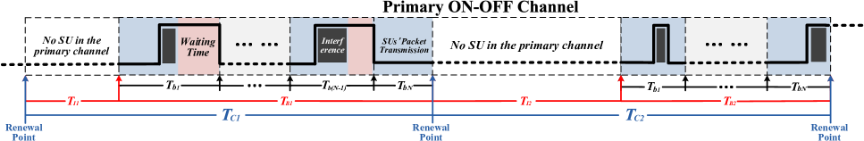
Figure 6: Illustration of the SUs’ idle-busy behavior in the primary channel when $\lambda_{s}\neq 0$.

Compared with the SUs’ behavior when $\lambda_{s}=0$, another state that may occur when $\lambda_{s}\neq 0$ is there is no SUs’ request in the coordinator’s buffer. We call this new state as an idle state of the SUs’ behavior, while the opposite busy state refers to the scenario when the coordinator’s buffer is not empty. The length of the idle state and busy state are denoted by $T_{I}$ and $T_{B}$ respectively. As shown in Fig. 6, the SUs’ behavior switches between the idle state and busy state, which is similar to the PU’s ON-OFF model. In the following, we prove that the SUs’ such idle-busy switching is also a renewal process.

Theorem 4: When the SUs’ transmission requests arrive by Poisson process with constant rate $\lambda_{s}^{-1}$, the SUs’ communication behavior is a renewal process in the primary channel.

Proof:

In Fig. 6, we use $T_{c}$ to denote one cycle of the SUs’ idle and busy state, i.e., $T_{c}=T_{I}+T_{B}$. To prove Theorem 4, we need to show that all cycles $T_{c1}$, $T_{c2}$, …are i.i.d.

For each idle state, its length $T_{I}=\widehat{T}_{s}$ is the forward recurrence time of the SUs’ arrival interval $T_{s}$ defined in Section III-B. Since the SUs’ requests arrive by Poisson process, $T_{I}\sim\frac{1}{\lambda_{s}}e^{-t/\lambda_{s}}$ according to the Renewal Theory [19]. Therefore, the lengths of all idle states are i.i.d. For each busy state, $T_{B}=\sum\limits_{i=1}^{N}T_{bi}$ as shown in Fig. 6, where $N$ is the number of SUs’ transmitting-waiting times during the busy state. Since all $T_{bi}$ are i.i.d as proved in Theorem 1, $T_{B1}$, $T_{B2}$, …will also be i.i.d if we can prove that the $N$ of all busy states are i.i.d. It is obvious that the $N$ of all busy states are independent since the SUs’ requests arrive by a Poisson process. In the following, we will focus on proving its property of identical distribution.

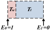
(a) $N=1$.

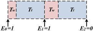
(b) $N=2$.

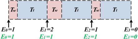
(c) $N=3$.

Figure 7: Illustration of buffer status $E_{l}$ when $N=1,2,3$.

To obtain the general distribution expression of $N$, we start from analyzing the cases with $N=1$, $2$, $3$ in Fig. 7, where $E_{l}$ represents the number of requests waiting in the coordinator’s buffer at the end of the $l$th $T_{t}$, i.e., the time right after the transmission of the SUs’ $l$th packet. Thus, as shown in Fig. 7-(a), the probability $P(N=1)$ is

$$P(N=1)=P(E_{1}=0|E_{0}=1)=P_{10},$$ (29)

where $P_{ij}$ denotes the probability that the last $T_{t}$ ends with $i$ requests in the coordinator’s buffer and current $T_{t}$ ends with $j$ requests. More specifically, $P_{ij}$ represents the probability that there are $j-i+1$ requests arriving at the coordinator during the period $T_{w}+T_{t}$. Since the SUs’ requests arrive by a Poisson process with arrival interval $T_{s}$, $P_{ij}$ can be calculated by

$$P_{ij} = P\Bigg{(}\sum\limits_{k=1}^{j-i+1}T_{s_{k}}\leq(T_{w}+T_{t})\leq\sum\limits_{k=1}^{j-i+2}T_{s_{k}}\Bigg{)}=\int_{T_{t}}^{+\infty}\frac{(t/\lambda_{s})^{j-i+1}}{(j-i+1)!}e^{-t/\lambda_{s}}P(T_{w}+T_{t}=t)dt,$$ (30)

$$= \int_{0}^{+\infty}\frac{\Big{(}(t+T_{t})/\lambda_{s}\Big{)}^{j-i+1}}{(j-i+1)!}e^{-(t+T_{t})/\lambda_{s}}P(T_{w}=t)dt,$$

where $T_{s_{k}}$ is the SUs’ $k$th arrival interval satisfying the exponential distribution with parameter $\lambda_{s}$, the first equality is because $\sum\limits_{k=1}^{j-i+1}T_{s_{k}}$ and $\sum\limits_{k=1}^{j-i+2}T_{s_{k}}$ satisfy Erlang distribution.

According to (4) and (26), the probability distribution of $T_{w}$, $P(T_{w}=t)$, can be written as follows

$$P(T_{w}=t)=\left\{\begin{array}[]{l}P_{\mbox{\tiny{OFF}}}(T_{t})_{\quad}\quad\quad\quad\ t=0,\vspace{2mm}\\ \frac{P_{\mbox{\tiny{ON }}}(T_{t})}{\lambda_{1}}e^{-t/\lambda_{1}}\quad\quad t>0,\end{array}\right.\$$ (31)

where $P_{\mbox{\tiny{OFF}}}(T_{t})=1-P_{\mbox{\tiny{ON}}}(T_{t})=\frac{\lambda_{0}}{\lambda_{0}+\lambda_{1}}\Big{(}1-e^{-\frac{\lambda_{0}+\lambda_{1}}{\lambda_{0}\lambda_{1}}T_{t}}\Big{)}$.

By substituting (31) into (30) , we can re-write $P_{ij}$ as

$$P_{ij}=P_{\mbox{\tiny{OFF}}}(T_{t})\cdot\frac{(T_{t}/\lambda_{s})^{j-i+1}}{(j-i+1)!}e^{-T_{t}/\lambda_{s}}+\int_{0^{+}}^{+\infty}\frac{\Big{(}(t+T_{t})/\lambda_{s}\Big{)}^{j-i+1}}{(j-i+1)!}\frac{P_{\mbox{\tiny{ON }}}(T_{t})}{\lambda_{1}}e^{-\big{(}\frac{\lambda_{1}+\lambda_{s}}{\lambda_{1}\lambda_{s}}t+T_{t}/\lambda_{s}\big{)}}dt.$$ (32)

When $N=2$, as shown in Fig. 7-(b), $P(N=2)$ can be written by

$$P(N=2)=P(E_{2}=0,E_{1}=1|E_{0}=1).$$ (33)

According to the queuing theory [27], the sequence $E_{1}$, $E_{2}$, …, $E_{N}$ is an embedded Markov process. Thus, $P(N=2)$ can be re-written by

$$P(N=2)=P(E_{1}=1|E_{0}=1)P(E_{2}=0|E_{1}=1)=P_{11}P_{10}.$$ (34)

When $N=3$, as shown in Fig. 7-(c), there are two cases ($E_{0}=1$, $E_{1}=2$, $E_{2}=1$, $E_{2}=0$) and ($E_{0}=1$, $E_{1}=1$, $E_{2}=1$, $E_{2}=0$). Thus,

$$P(N=3)=P_{12}P_{21}P_{10}+P_{11}P_{11}P_{10}.$$ (35)

When $N=n$, $E_{l}\ (0\leq l\leq n)$ should satisfy the following condition

$$E_{0}=1,\quad 1\leq E_{1}\leq n-1,\quad\dots,\quad 1\leq E_{l}\leq n-l,\quad\dots,\quad E_{n-1}=1,\quad E_{n}=0.$$ (36)

Thus, there are $(n-1)!$ possible combinations of ($E_{0}$, $E_{1}$, …, $E_{l}$, …, $E_{n-1}$, $E_{n}$). We denote each case as $C(a)$, where $1\leq a\leq(n-1)!$. For each case, the probability is the product of $n$ terms $P_{ij}\big{(}C(a),b\big{)}$, where $1\leq b\leq n$. Thus, $P(N=n)$ can be expressed as follows

$$P(N=n)=\sum\limits_{a=1}^{(n-1)!}\prod\limits_{b=1}^{n}P_{ij}\big{(}C(a),b\big{)}.$$ (37)

From (37), we can see that $N$ of all busy states are identical distributed, and hence i.i.d.

Up to now, we have come to the conclusion that $T_{I}$ of all idle states are i.i.d, as well as $T_{B}$ of all busy states. Since $T_{I}$ and $T_{B}$ are independent with each other, the sequence of all cycles’ lengths $T_{c1}$, $T_{c2}$, …are $i.i.d$. Therefore, the SUs’ communication behavior is a renewal process. ∎

V-B Interference Quantity Analysis

According to Definition 1 and Theorem 4, the interference quantity $Q_{I_{2}}$ can be calculated by

$$Q_{I_{2}}=\mu_{B}\cdot Q_{I_{1}},$$ (38)

where $\mu_{B}=\frac{\mathbb{E}(T_{B})}{\mathbb{E}(T_{I})+\mathbb{E}(T_{B})}$ is the occurrence probability of the SUs’ busy state.

Our system can be treated as an $M/G/1$ queuing system, where the customers are the SUs’ data packets and the server is the primary channel. The service time $S$ of one SU is the sum of its transmission time $T_{t}$ and the waiting time of the next SU $T_{w}$. In such a case, the expected service time is $\mathbb{E}(S)=T_{t}+\mathbb{E}(T_{w})$. According to the queuing theory [27], the load of the server is $\rho=\mathbb{E}(S)/\lambda$, where $\lambda$ is the average arrival interval of the customers. By Little’s law [27], $\rho$ is equivalent to the expected number of customers in the server. In our system, there can be at most one customer (SUs’ one packet) in the server, which means the expected number of customers is equal to the probability that there is a customer in the server. Therefore, $\rho$ is equal to the proportion of time that the coordinator is busy, i.e.,

$$\rho=\frac{T_{t}+\mathbb{E}(T_{w})}{\lambda_{s}}=\mu_{B}=\frac{\mathbb{E}(T_{B})}{\mathbb{E}(T_{I})+\mathbb{E}(T_{B})}.$$ (39)

Thus, combining (28), (38) and (39), the close-form expression of $Q_{I_{2}}$ can be obtained as follows

$$Q_{I_{2}}=\frac{(\lambda_{0}+\lambda_{1})T_{t}-\lambda_{0}\lambda_{1}\Big{(}1-e^{-\frac{\lambda_{0}+\lambda_{1}}{\lambda_{0}\lambda_{1}}T_{t}}\Big{)}}{\lambda_{s}(\lambda_{0}+\lambda_{1})}.$$ (40)

VI Optimizing Secondary Users’ Communication Performance

In this section, we will discuss how to optimize the SUs’ communication performance while maintaining the PU’s communication QoS and the stability of the secondary network. In our system, the SUs’ communication performance is directly dependent on the expected arrival interval of their packets $\lambda_{s}$ and the length of the transmission time $T_{t}$. These two important parameters should be appropriately chosen so as to minimize the interference caused by the SUs’ dynamic access and also to maintain a stable secondary network.

We consider two constraints for optimizing the SUs’ $\lambda_{s}$ and $T_{t}$ as follows

• the PU’s average data rate should be at least $R_{p}^{\downarrow}$,

• the stability condition of the secondary network should be satisfied.

In the following, we will first derive the expressions for these two constraints based on the analysis in Section IV and V. Then we formulate the problem of finding the optimal $\lambda_{s}^{\ast}$ and $T_{t}^{\ast}$ as an optimization problem to maximize the SUs’ average data rate.

VI-A The Constraints

VI-A1 PU’s Average Data Rate

If there is no interference from the SUs, the PU’s instantaneous rate is $\mbox{{log}}(1+\mbox{SNR}_{p})$, where $\mbox{SNR}_{p}$ denotes the Signal-to-Noise Ratio of primary signal at the PU’s receiver. On the other hand, if the interference occurs, the PU’s instantaneous rate will be $\mbox{{log}}\Big{(}1+\frac{\mbox{SNR}_{p}}{\mbox{INR}_{p}+1}\Big{)}$, where $\mbox{INR}_{p}$ is the Interference-to-Noise Ratio of secondary signal received by the PU. According to Definition 1, $Q_{I_{2}}$ represents the ratio of the interference periods to the PU’s overall communication time. Thus, the PU’s average data rate $R_{p}$ can be calculated by

$$R_{p}=\big{(}1-Q_{I_{2}}\big{)}\cdot\mbox{{log}}\Big{(}1+\mbox{SNR}_{p}\Big{)}+Q_{I_{2}}\cdot\mbox{{log}}\bigg{(}1+\frac{\mbox{SNR}_{p}}{\mbox{INR}_{p}+1}\bigg{)}.$$ (41)

VI-A2 SUs’ Stability Condition

In our system, the secondary network and the primary channel can be modeled as a single-server queuing system. According to the queuing theory [27], the stability condition for a single-server queue with Poisson arrivals is that the load of the server should satisfy $\rho<1$ [28]. In our system, we have

$$\rho=\frac{T_{t}+\mathbb{E}(T_{w})}{\lambda_{s}}<1.$$ (42)

In such a case, the SUs’ stability condition function, $S(T_{t},\lambda_{s})$, can be written as follows

$$S(T_{t},\lambda_{s})=\lambda_{s}-T_{t}-\frac{\lambda_{1}^{2}}{\lambda_{0}+\lambda_{1}}\Big{(}1-e^{-\frac{\lambda_{0}+\lambda_{1}}{\lambda_{0}\lambda_{1}}T_{t}}\Big{)}>0.$$ (43)

VI-B Objective Function: SUs’ Average Data Rate

If a SU encounters the PU’s recurrence, i.e., the ON state of the primary channel, during its transmission time $T_{t}$, its communication is also interfered by the PU’s signal. In such a case, the SU’s instantaneous rate is $\mbox{{log}}\Big{(}1+\frac{\mbox{SNR}_{s}}{\mbox{INR}_{s}+1}\Big{)}$, where $\mbox{SNR}_{s}$ is the SU’s Signal-to-Noise Ratio and $\mbox{INR}_{s}$ is the Interference-to-Noise Ratio of primary signal received by the SU. According to Theorem 1 and Theorem 4, the occurrence probability of such a phenomenon is $\mu_{B}\frac{I(T_{t})}{T_{t}+\mathbb{E}(T_{w})}=\frac{I(T_{t})}{\lambda_{s}}$. On the other hand, if no PU appears during the SU’s transmission, its instantaneous rate will be $\mbox{{log}}(1+\mbox{SNR}_{s})$ and the corresponding occurrence probability is $\mu_{B}\frac{T_{t}-I(T_{t})}{T_{t}+\mathbb{E}(T_{w})}=\frac{T_{t}-I(T_{t})}{\lambda_{s}}$. Thus, the SU’s average data rate $R_{s}$ is

$$R_{s}=\frac{T_{t}-I(T_{t})}{\lambda_{s}}\cdot\mbox{{log}}\Big{(}1+\mbox{SNR}_{s}\Big{)}+\frac{I(T_{t})}{\lambda_{s}}\cdot\mbox{{log}}\bigg{(}1+\frac{\mbox{SNR}_{s}}{\mbox{INR}_{s}+1}\bigg{)}.$$ (44)

VI-C Optimizing SUs’ Communication Performance

Based on the analysis of constraints and objective function, the problem of finding optimal $T_{t}^{\ast}$ and $\lambda_{s}^{\ast}$ for the SUs can be formulated as follows

$$\max\limits_{(T_{t},\lambda_{s})} R_{s}(T_{t},\lambda_{s})=\frac{T_{t}-I(T_{t})}{\lambda_{s}}\cdot\mbox{{log}}\Big{(}1+\mbox{SNR}_{s}\Big{)}+\frac{I(T_{t})}{\lambda_{s}}\cdot\mbox{{log}}\bigg{(}1+\frac{\mbox{SNR}_{s}}{\mbox{INR}_{s}+1}\bigg{)},$$

s.t. $$R_{p}(T_{t},\lambda_{s})=\big{(}1-Q_{I_{2}}\big{)}\cdot\mbox{{log}}\Big{(}1+\mbox{SNR}_{p}\Big{)}+Q_{I_{2}}\cdot\mbox{{log}}\bigg{(}1+\frac{\mbox{SNR}_{p}}{\mbox{INR}_{p}+1}\bigg{)}\geq R_{p}^{\downarrow},$$

$$\ S(T_{t},\lambda_{s})=\lambda_{s}-T_{t}-\frac{\lambda_{1}^{2}}{\lambda_{0}+\lambda_{1}}\Big{(}1-e^{-\frac{\lambda_{0}+\lambda_{1}}{\lambda_{0}\lambda_{1}}T_{t}}\Big{)}>0.$$

Theorem 5: The SUs’ average data rate $R_{s}(T_{t},\lambda_{s})$ is a strictly increasing function in terms of the their transmission time $T_{t}$ and a strictly decreasing function in terms of their average arrival interval $\lambda_{s}$, i.e.,

$$\frac{\partial{R_{s}}}{\partial{T_{t}}}>0,\quad\frac{\partial{R_{s}}}{\partial{\lambda_{s}}}<0.$$ (46)

The PU’s average data rate $R_{p}(T_{t},\lambda_{s})$ is a strictly decreasing function in terms of $T_{t}$ and a strictly increasing function in terms of $\lambda_{s}$, i.e.,

$$\frac{\partial{R_{p}}}{\partial{T_{t}}}<0,\quad\frac{\partial{R_{p}}}{\partial{\lambda_{s}}}>0.$$ (47)

The stability condition function $S(T_{t},\lambda_{s})$ is a strictly decreasing function in terms of $T_{t}$ and a strictly increasing function in terms of $\lambda_{s}$, i.e.,

$$\frac{\partial{S}}{\partial{T_{t}}}<0,\quad\frac{\partial{S}}{\partial{\lambda_{s}}}>0.$$ (48)

Proof:

For simplification, we use $R_{s0}$ to express $\mbox{{log}}\Big{(}1+\mbox{SNR}_{s}\Big{)}$ and $R_{s1}$ to express $\mbox{{log}}\bigg{(}\!1+\frac{\mbox{SNR}_{s}}{\mbox{INR}_{s}+1}\!\bigg{)}$. According to (44) and (18), $\frac{\partial{R_{s}}}{\partial{T_{t}}}$ and $\frac{\partial{R_{s}}}{\partial{\lambda_{s}}}$ can be calculated as follows

$$\frac{\partial{R_{s}}}{\partial{T_{t}}} = \frac{R_{s0}}{\lambda_{s}}-\frac{R_{s0}-R_{s1}}{\lambda_{s}}\cdot\frac{\partial{I(T_{t})}}{\partial{T_{t}}},$$ (49)

$$= \frac{1}{\lambda_{s}(\lambda_{0}+\lambda_{1})}\bigg{(}\lambda_{0}R_{s0}+\lambda_{1}R_{s1}+\lambda_{1}(R_{s0}-R_{s1})\Big{(}1-e^{-\frac{\lambda_{0}+\lambda_{1}}{\lambda_{0}\lambda_{1}}T_{t}}\Big{)}\bigg{)},$$

$$\frac{\partial{R_{s}}}{\partial{\lambda_{s}}} = -\frac{1}{\lambda^{2}_{s}}\bigg{(}\Big{(}T_{t}-I(T_{t})\Big{)}R_{s0}+I(T_{t})R_{s1}\bigg{)}.$$ (50)

Since $R_{s0}>R_{s1}$, $e^{-\frac{\lambda_{0}+\lambda_{1}}{\lambda_{0}\lambda_{1}}T_{t}}<1$, and $T_{t}\geq I(T_{t})$, we have

$$\frac{\partial{R_{s}}}{\partial{T_{t}}}>0,\quad\frac{\partial{R_{s}}}{\partial{\lambda_{s}}}<0.$$ (51)

Similarly, we use $R_{p0}$ to express $\mbox{{log}}\Big{(}1+\mbox{SNR}_{p}\Big{)}$ and $R_{p1}$ to express $\mbox{{log}}\bigg{(}1+\frac{\mbox{SNR}_{p}}{\mbox{INR}_{p}+1}\bigg{)}$. According to (41), $\frac{\partial{R_{p}}}{\partial{T_{t}}}$ and $\frac{\partial{R_{p}}}{\partial{\lambda_{s}}}$ can be calculated as follows

$$\frac{\partial{R_{p}}}{\partial{T_{t}}}=-\frac{\partial{Q_{I_{2}}}}{\partial{T_{t}}}(R_{s0}-R_{s1}),\quad\frac{\partial{R_{p}}}{\partial{\lambda_{s}}}=-\frac{\partial{Q_{I_{2}}}}{\partial{\lambda_{s}}}(R_{s0}-R_{s1}).$$ (52)

According to (40), we have

$$\frac{\partial{Q_{I_{2}}}}{\partial{T_{t}}}=\frac{1-e^{-\frac{\lambda_{0}+\lambda_{1}}{\lambda_{0}\lambda_{1}}T_{t}}}{\lambda_{s}}>0,\quad\frac{\partial{Q_{I_{2}}}}{\partial{\lambda_{s}}}<0.$$ (53)

Thus, combining (52) and (53), we have

$$\frac{\partial{R_{p}}}{\partial{T_{t}}}<0,\quad\frac{\partial{R_{p}}}{\partial{\lambda_{s}}}>0.$$ (54)

According to (43), $\frac{\partial{S}}{\partial{T_{t}}}$ and $\frac{\partial{S}}{\partial{\lambda_{s}}}$ can be calculated as follows

$$\frac{\partial{S}}{\partial{T_{t}}}=-\bigg{(}1+\frac{\lambda_{1}}{\lambda_{0}}e^{-\frac{\lambda_{0}+\lambda_{1}}{\lambda_{0}\lambda_{1}}T_{t}}\bigg{)}<0,\quad\frac{\partial{S}}{\partial{\lambda_{s}}}=1>0.$$ (55)

This completes the proof of the theorem. ∎

From Theorem 5, we can see that the objective function and the constraints are all monotonous functions in terms of $T_{t}$ and $\lambda_{s}$. Thus, the solution to the optimization problem (VI-C) can be found using gradient descent method [29].

VII Simulation Results

In this section, we conduct simulations to verify the effectiveness of our analysis. The parameters of primary ON-OFF channel are set to be $\lambda_{0}=2.6$s and $\lambda_{1}=3.6$s. According to Fig. 3, we build a queuing system using Matlab to simulate the PU’s and SUs’ behaviors.

VII-A Interference Quantity $Q_{I}$

In Fig. 9 and Fig. 9, we illustrate the theoretic and simulated results of $Q_{I_{1}}$ and $Q_{I_{2}}$, respectively. The theoretic $Q_{I_{1}}$ and $Q_{I_{2}}$ are computed according to (28) and (40) with different values of the SUs’ transmission time $T_{t}$. The average arrival interval of the SUs’ packets $\lambda_{s}$ is set to be $1.3$s when calculating theoretic $Q_{I_{2}}$. For the simulated results, once the interference occurs, we calculate and record the ratio of the accumulated interference periods to the accumulated periods of the ON states.

From Fig. 9 and Fig. 9, we can see that all the simulated results of $Q_{I_{1}}$ and $Q_{I_{2}}$ eventually converge to the corresponding theoretic results after some fluctuations at the beginning, which means that the close-form expressions in (28) and (40) are correct and can be used to calculate the interference caused by the SUs in the practical cognitive radio system. Moreover, we can also see that the interference increases as the SUs’ transmission time $T_{t}$ increases. Such a phenomenon is because the interference to the PU can only occur during $T_{t}$ and the increase of $T_{t}$ enlarges the occurrence probability of $T_{t}$. Finally, we find that due to the existence of the idle state when $\lambda_{s}\neq 0$, $Q_{I_{2}}$ is less than $Q_{I_{1}}$ under the same condition.

VII-B Stability of The Secondary Network

Since we have modeled the secondary network as a queuing system shown in Fig. 3, the stability of the network is reflected by the status of the coordinator’s buffer. A stable network means that the requests waiting in the coordinator’s buffer do not explode as time goes to infinite, while the requests in the buffer of an unstable network will eventually go to infinite. In Section VI-A2, we have shown the stability condition of the secondary network in (43). On one hand, if the SUs’ access time $T_{t}$ is given in advance, the SUs’ minimal average arrival interval $\lambda_{s}$ can be computed by (43). On the other hand, if $\lambda_{s}$ is given, the maximal $T_{t}$ can be obtained to restrict the SUs’ transmission time.

In this simulation, we set $T_{t}=0.6$s, and thus $\lambda_{s}$ should be larger than $1.25$s to ensure the SUs’ stability according to (43). In Fig. 9, we show the queuing length, i.e., the number of requests in the coordinator’s buffer, versus the time. The black lines shows the queuing length of a stable network, in which $\lambda_{s}=1.3$s is larger than the threshold $1.25$s. It can be seen that the requests dynamically vary between $0$ and $60$. However, if we set $\lambda_{s}=1.2$s, which is smaller than the lower limit, from Fig. 9, we can see that the queuing length will finally go to finite, which represents an unstable network. Therefore, the stability condition in (43) should be satisfied to maintain a stable secondary network.

VII-C PU’s and SUs’ Average Data Rate

The simulation results of the PU’s average data rate $R_{p}$ versus the SUs’ transmission time $T_{t}$ and arrival interval $\lambda_{s}$ are shown in Fig. 12, where we set $\mbox{SNR}_{p}\!=\!\mbox{SNR}_{s}\!=\!5$db and $\mbox{INR}_{p}\!=\!\mbox{INR}_{s}\!=\!3$db. We can see that $R_{p}$ is a decreasing function in terms of $T_{t}$ given a certain $\lambda_{s}$, and an increasing function in terms of $\lambda_{s}$ for any fixed $T_{t}$, which is in accordance with Theorem 5. Such a phenomenon is because an increase of $T_{t}$ or a decrease of $\lambda_{s}$ will cause more interference to the PU and thus degrade its average data rate. In Fig. 12, we illustrate the simulation results of the SUs’ average data rate $R_{s}$ versus $T_{t}$ and $\lambda_{s}$. Different from $R_{p}$, $R_{s}$ is an increasing function in terms of $T_{t}$ given a certain $\lambda_{s}$, and a decreasing function in terms of $\lambda_{s}$ for any fixed $T_{t}$, which also verifies the correctness of Theorem 5.

Suppose that the PU’s data rate should be at least $2.0$bps/Hz, i.e., $R_{p}^{\downarrow}=2.0$bps/Hz. Then, according to the constraints in (VI-C), $T_{t}$ should be no larger than the location of those three colored vertical lines in Fig. 12 corresponding to $\lambda_{s}=1.3$s, $1.5$s, $2.0$s respectively. For example, when $\lambda_{s}=1.3$s, the optimal $T_{t}^{\ast}$ should be around $400$ms to satisfy both the $R_{p}^{\downarrow}$ and stability condition constraints. In such a case, the SUs’ average data rate can achieve around $0.6$bps/Hz according to Fig. 12. For any fixed $R_{p}^{\downarrow}$, the optimal values of $T_{t}^{\ast}$ and $\lambda_{s}^{\ast}$ are determined by the channel parameters $\lambda_{0}$ and $\lambda_{1}$. Therefore, the SUs should dynamically adjust their communication behaviors according to the estimated channel parameters.

VIII Conclusion

In this paper, we analyzed the interference caused by the SUs confronted with unknown primary behavior. Based on the Renewal Theory, we showed that the SUs’ communication behaviors in the ON-OFF primary channel is a renewal process and derived the close-form for the interference quantity. We further discussed how to optimize the SUs’ arrival rate and transmission time to control the level of interference to the PU and maintain the stability of the secondary network. Simulation results are shown to validate our close-form expressions for the interference quantity. In the practical cognitive radio networks, these expressions can be used to evaluate the interference from the SUs when configuring the secondary network. In the future work, we will study how to concretely coordinate the primary spectrum sharing among multiple SUs.

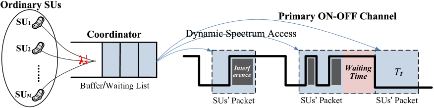
Figure 3: Illustration of the queuing system, the SUs’ dynamic spectrum access and interference to the PU.

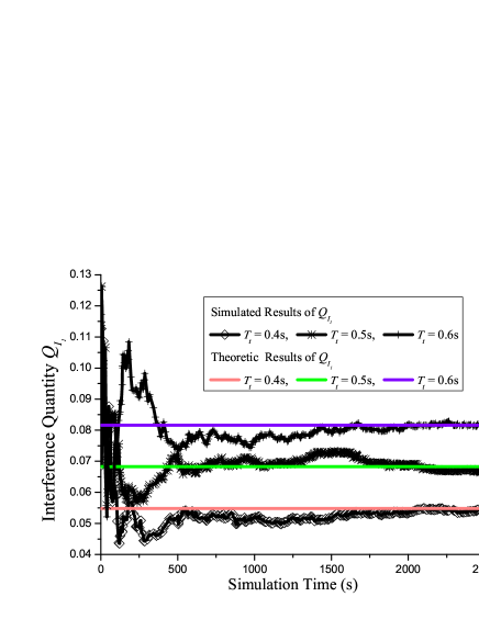
Figure 8: Interference quantity $Q_{I_{1}}$.

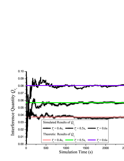
Figure 9: Interference quantity $Q_{I_{2}}$ with $\lambda_{s}=1.3$s.

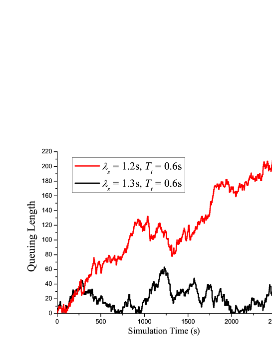
Figure 10: Queuing length under stable and unstable conditions.

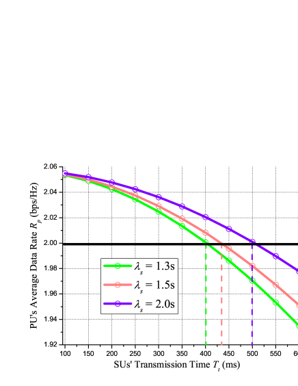
Figure 11: PU’s average data rate.

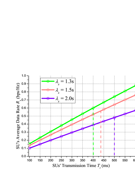
Figure 12: SUs’ average data rate.

References

- [1] S. Haykin, “Cognitive radio: brain-empowered wireless communications,” IEEE J. Sel. Areas Commun., vol. 23, no. 2, pp. 201–220, 2005.
- [2] K. J. R. Liu and B. Wang, Cognitive Radio Networking and Security: A Game Theoretical View. Cambridge University Press, 2010.
- [3] B. Wang and K. J. R. Liu, “Advances in cognitive radios: A survey,” IEEE J. Sel. Topics Signal Process., vol. 5, no. 1, pp. 5–23, 2011.
- [4] B. Wang, Z. Ji, K. J. R. Liu, and T. C. Clancy, “Primary-prioritized markov approach for efficient and fair dynamic spectrum allocation,” IEEE Trans. Wireless Commun., vol. 8, no. 4, pp. 1854–1865, 2009.
- [5] Z. Chen, C. Wang, X. Hong, J. Thompson, S. A. Vorobyov, and X. Ge, “Interference modeling for cognitive radio networks with power or contention control,” in Proc. IEEE WCNC, 2010, pp. 1–6.
- [6] G. L. Stuber, S. M. Almalfouh, and D. Sale, “Interference analysis of TV band whitespace,” Proc. IEEE, vol. 97, no. 4, pp. 741–754, 2009.
- [7] M. Vu, D. Natasha, and T. Vahid, “On the primary exclusive regions in cognitive networks,” IEEE Trans. Wireless Commun., vol. 8, no. 7, pp. 3380–3385, 2008.
- [8] R. S. Dhillon and T. X. Brown, “Models for analyzing cognitive radio interference to wireless microphones in TV bands,” in Proc. IEEE DySPAN, 2008, pp. 1–10.
- [9] M. Timmers, S. Pollin, A. Dejonghe, A. Bahai, L. V. Perre, and F. Catthoor, “Accumulative interference modeling for cognitive radios with distributed channel access,” in Proc. IEEE CrownCom, 2008, pp. 1–7.
- [10] R. Menon, R. M. Buehrer, and J. H. Reed, “Outage probability based comparison of underlay and overlay spectrum sharing techniques,” in Proc. IEEE DySPAN, 2005, pp. 101–109.
- [11] ——, “On the impact of dynamic spectrum sharing techniques on legacy radio systems,” IEEE Trans. Wireless Commun., vol. 7, no. 11, pp. 4198–4207, 2008.
- [12] M. F. Hanif, M. Shafi, P. J. Smith, and P. Dmochowski, “Interference and deployment issues for cognitive radio systems in shadowing environments,” in Proc. IEEE ICC, 2009, pp. 1–6.
- [13] A. Ghasemi and E. S. Sousa, “Interference aggregation in spectrum-sensing cognitive wireless networks,” IEEE J. Sel. Topics Signal Process., vol. 2, no. 1, pp. 41–56, 2008.
- [14] A. K. Sadek, K. J. R. Liu, , and A. Ephremides, “Cognitive multiple access via cooperation: protocol design and stability analysis,” IEEE Trans. Inform. Theory, vol. 53, no. 10, pp. 3677–3696, 2007.
- [15] A. A. El-Sherif, A. Kwasinski, A. Sadek, and K. J. R. Liu, “Content-aware cognitive multiple access protocol for cooperative packet speech communications,” IEEE Trans. Wireless Commun., vol. 8, no. 2, pp. 995–1005, 2009.
- [16] A. A. El-Sherif, A. K. Sadek, and K. J. R. Liu, “Opportunistic multiple access for cognitive radio networks,” IEEE J. Sel. Areas Commun., vol. 29, no. 4, pp. 704–715, 2011.
- [17] A. A. El-Sherif and K. J. R. Liu, “Joint design of spectrum sensing and channel access in cognitive radio networks,” IEEE Trans. Wireless Commun., vol. 10, no. 6, pp. 1743–1753, 2011.
- [18] Y.-C. Liang, Y. Zeng, E. C. Peh, and A. T. Hoang, “Sensing-throughput tradeoff for cognitive radio networks,” IEEE Trans. Wireless Commun., vol. 7, no. 4, pp. 1326–1337, 2008.
- [19] D. R. Cox, Renewal Theory. Butler and Tanner, 1967.
- [20] H. Kim and K. G. Shin, “Efficient discovery of spectrum opportunities with MAC-layer sensing in cognitive radio networks,” IEEE Trans. Mobile Computing, vol. 7, no. 5, pp. 533–545, 2008.
- [21] D. Xue, E. Ekici, and X. Wang, “Opportunistic periodic MAC protocol for cognitive radio networks,” in Proc. IEEE GLOBECOM, 2010, pp. 1–6.
- [22] P. K. Tang and Y. H. Chew, “Modeling periodic sensing errors for opportunistic spectrum access,” in Proc. IEEE VTC-FALL, 2010, pp. 1–5.
- [23] M. Sharma, A. Sahoo, and K. D. Nayak, “Model-based opportunistic channel access in dynamic spectrum access networks,” in Proc. IEEE GLOBECOM, 2009, pp. 1–6.
- [24] S. Wang, W. Wang, F. Li, and Y. Zhang, “Anticipated spectrum handover in cognitive radios,” in Proc. IEEE ICT, 2011, pp. 49–54.
- [25] P. Wang and I. F. Akyildiz, “On the origins of heavy tailed delay in dynamic spectrum access networks,” accepted by IEEE Trans. Mobile Comput., 2011.
- [26] R. Chen and X. Liu, “Delay performance of threshold policies for dynamic spectrum access,” IEEE Trans. Wireless Commun., vol. 10, no. 7, pp. 2283–2293, 2011.
- [27] D. Gross, J. F. Shortle, J. M. Thompson, and C. M. Harris, Fundamentals of Queueing Theory. Wiley, 2008.
- [28] H.-M. Liang and V. G. Kulkarni, “Stability condition for a single-server retrial queue,” Adv. Appl. Prob., vol. 25, no. 3, pp. 690–701, 1993.
- [29] D. P. Bertsekas, Nonlinear Programming. Athena Scientific, 1999.