Eigenvalue comparison on Bakry-Emery manifolds

1. A lower bound for the first eigenvalue of the drift Laplacian

Recall that $(M,g,f)$, a triple consisting of a manifold $M$, a Riemannian metric $g$ and a smooth function $f$, is called a gradient Ricci soliton if the Ricci curvature and the Hessian of $f$ satisfy:

(1.1) $${\rm Rc}_{ij}+f_{ij}=ag_{ij}.$$

It is called shrinking, steady, or expanding soliton if $a>0$, $a=0$ or $a<0$ respectively. In this paper we apply the modulus of continuity estimates developed in [AC1, AC2, AC3] to give an eigenvalue estimate on gradient solitons for the operator $\Delta_{f}\doteqdot\Delta-\langle\nabla(\cdot),\nabla f\rangle$ on strictly convex $\Omega\subset M$ with diameter $D$ and smooth boundary. In fact the result works for manifolds with lower bound on the so-called Bakry-Emery Ricci tensor, namely ${\rm Rc}_{ij}+f_{ij}\geq ag_{ij}$ for some $a\in\mathbb{R}$. An earlier result of this kind was obtained in [FS] for shrinking solitons.

In this section, we extend a comparison theorem of [AC3] on the modulus of continuity to manifolds with lower bound on the co-called Bakry-Emery Ricci tensor. The eigenvalue comparison result for manifolds with lower bound on the Bakry-Emery tensor generalizes the earlier lower estimates of Payne-Weinberger[PW], Li-Yau[LY] and Zhong-Yang[ZY]. A consequence of this is a lower diameter estimate for nontrivial gradient shrinking solitons, which improves [FS] with a different approach and a rather short argument. We remark here that the eigenvalue estimate we obtain is sharp for $(M,g,f)$ satisfying the Bakry-Emery-Ricci lower bound ${\rm Rc}_{ij}+f_{ij}\geq ag_{ij}$, but presumably is not so for Ricci solitons where the Bakry-Emery-Ricci tensor is constant, and so we expect that our diameter bound is also not sharp. We discuss the sharpness of the eigenvalue inequality in section 2.

Before we state the result, we define a corresponding $1$-dimensional eigenvalue problem. On $[-\frac{D}{2},\frac{D}{2}]$ we consider the functionals

$$\mathcal{F}(\psi)=\int_{\frac{D}{2}}^{\frac{D}{2}}\mathrm{e}^{-\frac{a}{2}s^{2}}(\psi^{\prime})^{2}\,ds,\quad\text{ and }\quad\mathcal{R}(\psi)=\frac{\mathcal{F}(\psi)}{\int\mathrm{e}^{-\frac{a}{2}s^{2}}\psi^{2}ds},$$

namely the Dirichlet energy with weight $\mathrm{e}^{-\frac{a}{2}s^{2}}$ and its Rayleigh quotient. The associated elliptic operator is $\mathcal{L}_{a}=\frac{d^{2}}{ds^{2}}-a\,s\frac{d}{ds}$. Let $\bar{\lambda}_{a,D}$ be the first non-zero Neumann eigenvalue of $\mathcal{L}_{a}$, which is the minimum of $\mathcal{R}$ among $W^{1,2}$-functions with zero average.

Theorem 1.1.

Let $\Omega$ be a compact manifold $M$, or a bounded strictly convex domain inside a complete manifold $M$, satisfying that ${\rm Rc}_{ij}+f_{ij}\geq a\,g_{ij}$. Assume that $D$ is the diameter of $\Omega$. Then the first non-zero Neumann eigenvalue $\widetilde{\lambda}_{1}$ of the operator $\Delta_{f}$ is at least $\bar{\lambda}_{a,D}$.

Proof.

First we extend Theorem 2.1 of [AC3] to this setting. Recall that $\omega$ is a modulus of continuity for a function $f$ on $M$ if for all $x$ and $y$ in $M$, $|f(y)-f(x)|\leq 2\omega\left(\frac{d_{M}(x,y)}{2}\right)$.

Proposition 1.1.

Let $v(x,t)$ be a solution to

(1.2) $$\frac{\partial v}{\partial t}=\Delta v-2\langle X,\nabla v\rangle$$

with $2X=\nabla f$. Assume also $v(x,t)$ satisfies the Neumann boundary condition. Suppose that $v(x,0)$ has a modulus of continuity $\varphi_{0}(s):[0,\frac{D}{2}]\to\mathbb{R}$ with $\varphi_{0}(0)=0$ and $\varphi_{0}^{\prime}>0$ on $[0,\frac{D}{2}]$. Assume further that there exists a function $\varphi(s,t):[0,\frac{D}{2}]\times\mathbb{R}_{+}\to\mathbb{R}$ such that

• $\varphi(s,0)=\varphi_{0}(s)$ on $[0,D/2]$;

• $\frac{\partial\varphi}{\partial t}\geq\varphi^{\prime\prime}-a\,s\,\varphi^{\prime}$ on $[0,D/2]\times\mathbb{R}_{+}$;

• $\varphi^{\prime}(s,t)>0$ on $[0,\frac{D}{2}]$;

• $\varphi(0,t)\geq 0$ for each $t\geq 0$.

Then $\varphi(s,t)$ is a modulus of the continuity of $v(x,t)$ for $t>0$.

The proof to the proposition is a modification of the argument to Theorem 2.1 of [AC3]. Precisely, consider

$$\mathcal{O}_{\epsilon}(x,y,t)\doteqdot v(y,t)-v(x,t)-2\varphi\left(\frac{r(x,y)}{2},t\right)-\epsilon\mathrm{e}^{t}$$

and it suffices to prove that the maximum of $\mathcal{O}_{\epsilon}(\cdot,\cdot,t)$ is non-increasing in $t$. The strictly convexity, the Neumann boundary condition satisfied by $v(x,t)$, and the positivity of $\varphi^{\prime}$ rule out the possibility that the maximum can be attained at $(x_{0},y_{0})\in\partial(\Omega\times\Omega)$. For the interior pair $(x_{0},y_{0})$ where the maximum of $\mathcal{O}_{\epsilon}(\cdot,\cdot,t)>0$ is attained, pick a frame $\{e_{i}\}$ as before at $x_{0}$ and parallel translate it along a minimizing geodesic $\gamma(s):[0,d]\to M$ joining $x_{0}$ with $y_{0}$. Still denote it by $\{e_{i}\}$. Let $\{E_{i}\}$ be the frame at $(x_{0},y_{0})$ (in $T_{(x_{0},y_{0})}\Omega\times\Omega$) as in Section 2. Direct calculations show that at $(x_{0},y_{0})$,

$$\left(\frac{\partial}{\partial t}-\sum_{j=1}^{n}\nabla^{2}_{E_{j}E_{j}}\right)\mathcal{O}_{\epsilon}(x,y,t) = -\left(\langle\nabla f(y),\gamma^{\prime}\rangle-\langle\nabla f(x),\gamma^{\prime}\rangle\right)\varphi^{\prime}$$

$$+\varphi^{\prime}\sum_{i=1}^{n-1}\nabla^{2}_{E_{i}E_{i}}r(x,y)-2\varphi_{t}+2\varphi^{\prime\prime}-\epsilon\mathrm{e}^{t}.$$

Here we have used the first variation $\nabla\mathcal{O}(\cdot,\cdot,t)=0$ at $(x_{0},y_{0})$ which implies the identities

$$(\nabla v)(y,t)=\varphi^{\prime}\,\gamma^{\prime}(d),\quad\quad(\nabla v)(x,t)=\varphi^{\prime}\,\gamma^{\prime}(0).$$

Now choose the variational vector field $V_{i}(s)=e_{i}(s)$, the parallel transport of $e_{i}$ along $\gamma(s)$, along $\gamma(s)$, the second variation computation gives that

$$\sum_{i=1}^{n-1}\nabla^{2}_{E_{i}E_{i}}r(x,y)\leq-\int_{0}^{d}\operatorname{Rc}(\gamma^{\prime},\gamma^{\prime})\,ds.$$

Hence at $(x_{0},y_{0})$ we have that

$$\left(\frac{\partial}{\partial t}-\sum_{j=1}^{n}\nabla^{2}_{E_{j}E_{j}}\right)\mathcal{O}(x,y,t) \leq -\varphi^{\prime}\int_{0}^{d}(\nabla^{2}f+\operatorname{Rc})(\gamma^{\prime},\gamma^{\prime})\,ds-2\varphi_{t}+2\varphi^{\prime\prime}$$

$$\leq -\varphi^{\prime}ar(x,y)-2\varphi_{t}+2\varphi^{\prime\prime}$$

$$\leq 0.$$

Here we have used $d=r(x,y)$ and $s=\frac{r(x,y)}{2}$. This is enough to prove the proposition.

To prove the theorem, let $\bar{\omega}(s)$ be the first non-constant eigenfunction for $\mathcal{L}_{a}$, which can be chosen to be positive on $(0,\frac{D}{2})$. To apply the proposition we consider $\bar{\omega}^{D^{\prime}}(s)$ be the eigenfunction on $[-\frac{D^{\prime}}{2},\frac{D^{\prime}}{2}]$ with the corresponding eigenvalue $\bar{\lambda}_{a}^{D^{\prime}}$. Let $\varphi(x,t)=C\mathrm{e}^{-\bar{\lambda}^{D^{\prime}}_{a}t}\bar{\omega}^{D^{\prime}}(s)$. Let $w(x)$ be the first non-constant eigenfunction of $\Delta_{f}$ and let $v(x,t)=e^{-\widetilde{\lambda}_{1}t}w(x)$. Since $\bar{\omega}^{D^{\prime}}(s)$ is an odd function (by adding an eigenfunction $\psi(s)$ with $\psi(-s)$ one can always obtain one), we do have $\varphi(0,t)=0$. The possibility of choosing $(\bar{\omega}^{D^{\prime}})^{\prime}(s)>0$ on $[0,\frac{D}{2}]$ can be proved as follows. By the uniqueness, we have that $(\bar{\omega}^{D^{\prime}})^{\prime}(0)>0$. It suffices to show that $(\bar{\omega}^{D^{\prime}})^{\prime}(s)>0$ for $s\in(0,\frac{D^{\prime}}{2})$. Also observe that $\bar{\omega}^{D^{\prime}}(\frac{D^{\prime}}{2})>0$. By the ODE $\mathcal{L}_{a}\bar{\omega}^{D^{\prime}}=-\bar{\lambda}\bar{\omega}^{D^{\prime}}$ we can conclude that $(\bar{\omega}^{D^{\prime}})^{\prime}>0$ on $[\frac{D^{\prime}}{2}-\epsilon,\frac{D^{\prime}}{2})$. Let $y(s)=(\bar{\omega}^{D^{\prime}})^{\prime}(s)$. The ODE also forces $y>0$ for $s\in(0,\frac{D^{\prime}}{2})$ since otherwise we assume $s_{1}<\frac{D^{\prime}}{2}$ is the biggest zero. Note that $\bar{\omega}^{D^{\prime}}(s_{1})<0$ and it is strictly convex near $s_{1}$. Now clearly near $s_{1}$ one can raise the value of $\bar{\omega}^{D^{\prime}}$ by replacing part of the graph with a line interval parallel to the $x$-axis, hence lower the energy $\mathcal{F}$. This contradicts the fact that $\bar{\lambda}$ is the minimum of the quotient $\mathcal{R}(\psi)$ among all nonzero $W^{1,2}(\mathrm{e}^{-\frac{a}{2}s^{2}}ds)$ function with zero average.

Finally as before the proposition implies that for sufficient large $C$, $\varphi(s,t)$ is a modulus of continuity of $v(x,t)$. Hence $\widetilde{\lambda}_{1}\geq\bar{\lambda}_{a,D^{\prime}}$. The claimed result follows by letting $D^{\prime}\to D$. $\square$

2. Sharpness of the lower bound

In this section we show that (for $n\geq 3$ for any $a$ or for $n\geq 2$ for $a\leq 0$) the lower bound $\tilde{\lambda}_{1}\geq\bar{\lambda}_{a}$ given in Theorem 1.1 is sharp: Precisely, for each $\varepsilon>0$ we construct a Bakry-Emery manifold $(M,g,f)$ with diameter $D$ and $\tilde{\lambda}_{1}<\bar{\lambda}_{a,D}+\varepsilon$.

We will construct a smooth manifold $M$ which is approximately a thin cylinder with hemispherical caps at each end. Let $\gamma$ be the curve in $\mathbb{R}^{2}$ with curvature $k$ given as function of arc length as follows for suitably small positive $r$ and $\delta>0$ small compared to $r$:

(2.1) $$k(s)=\begin{cases}\frac{1}{r},&s\in\left[0,\frac{\pi r}{2}-\delta\right];\\ \varphi\left(\frac{s-\frac{\pi r}{2}}{\delta}\right)\frac{1}{r},&s\in\left[\frac{\pi r}{2}-\delta,\frac{\pi r}{2}+\delta\right];\\ 0,&s\in\left[\frac{\pi r}{2}+\delta,\frac{D}{2}\right],\end{cases}$$

extended to be even under reflection in both $s=0$ and $s=D/2$. This corresponds to a pair of line segments parallel to the $x$ axis, capped by semicircles of radius $r$ and smoothed at the joins. We write the corresponding embedding $(x(s),y(s))$. Here $\varphi$ is a smooth nonincreasing function with $\varphi(s)=1$ for $s\leq-1$, $\varphi(s)=0$ for $s\geq 1$, and satisfying $\varphi(s)+\varphi(-s)=1$. We choose the point corresponding to $s=0$ to have $y(0)=0$ and $y^{\prime}(0)=1$. The manifold $M$ will then be the hypersurface of rotation in $\mathbb{R}^{n+1}$ given by $\{(x(s),y(s)z):\ s\in\mathbb{R},\ z\in\mathbb{S}^{n-1}\}$. On $M$ we choose the function $f$ to be a function of $s$ only, such that

(2.2) $$f^{\prime\prime}=\begin{cases}a\left(1-\frac{D}{\pi r}\right),&s\in\left[0,\frac{\pi r}{2}-\delta\right];\\ \varphi\left(\frac{s-\frac{\pi r}{2}}{\delta}\right)a\left(1-\frac{D}{\pi r}\right)+\left(1-\varphi\left(\frac{s-\frac{\pi r}{2}}{\delta}\right)\right)a,&s\in\left[\frac{\pi r}{2}-\delta,\frac{\pi r}{2}+\delta\right];\\ a,&s\in\left[\frac{\pi r}{2}+\delta,\frac{D}{2}\right],\end{cases}$$

with $f^{\prime}(0)=0$ (the value of $f(0)$ is immaterial). Note that this choice gives $f^{\prime}(D/2)=0$. We extend $f$ to be even under reflection in $s=0$ and $s=D/2$.

With these choices we compute the Bakry-Emery-Ricci tensor and verify that the eigenvalues are no less than $a$ for suitable choice of $r$. The eigenvalues of the second fundamental form are $k(s)$ (in the $s$ direction) and $\frac{\sqrt{1-(y^{\prime})^{2}}}{y}$ in the orthogonal directions. Therefore the Ricci tensor has eigenvalues $(n-1)k\frac{\sqrt{1-(y^{\prime})^{2}}}{y}$ in the $s$ direction, and $k\frac{\sqrt{1-(y^{\prime})^{2}}}{y}+(n-2)\frac{1-(y^{\prime})^{2}}{y^{2}}$ in the orthogonal directions. We can also compute the eigenvalues of the Hessian of $f$: The curves of fixed $z$ in $M$ are geodesics parametrized by $s$, the the Hessian in this direction is just $f^{\prime\prime}$ as given above. Since $f$ depends only on $s$ we also have that $\nabla^{2}f(\partial_{s},e_{i})=0$ for $e_{i}$ tangent to $\mathbb{S}^{n-1}$, and $\nabla^{2}f(e_{i},e_{j})=\frac{y^{\prime}}{y}f^{\prime}\delta_{ij}$.

The identities $y(s)=\int_{0}^{s}\cos\left(\theta(\tau)\right)\,d\tau$ and $y^{\prime}(s)=\cos\left(\theta(s)\right)$ where $\theta(s)=\int_{0}^{s}k(\tau)\,d\tau$ applied to (2.1) imply that

$$y=\begin{cases}r\sin(s/r),&s\in\left[0,\frac{\pi r}{2}-\delta\right];\\ r(1+o(\delta)),&s\in\left[\frac{\pi r}{2}-\delta,\frac{D}{2}\right],\end{cases}\qquad y^{\prime}=\begin{cases}\cos(s/r),&s\in\left[0,\frac{\pi r}{2}-\delta\right];\\ o(\delta),&s\in\left[\frac{\pi r}{2}-\delta,\frac{\pi r}{2}+\delta\right];\\ 0,&s\in\left[\frac{\pi r}{2}+\delta,\frac{D}{2}\right],\end{cases}$$

as $\delta$ approaches zero. This gives the following expressions for the Bakry-Emery Ricci tensor $\text{\rm Rc}_{f}=\text{\rm Rc}+\nabla^{2}f$:

$$\text{\rm Rc}_{f}(\partial_{s},\partial_{s})=\begin{cases}a+\frac{n-1}{r^{2}}-\frac{aD}{\pi r},&s\in\left[0,\frac{\pi r}{2}-\delta\right];\\ a+\varphi\left(\frac{2-\frac{\pi r}{2}}{\delta}\right)\left(\frac{n-1}{r^{2}}(1+o(\delta))-\frac{aD}{\pi r}\right)&s\in\left[\frac{\pi r}{2}-\delta,\frac{\pi r}{2}+\delta\right];\\ a,&s\in\left[\frac{\pi r}{2}+\delta,\frac{D}{2}\right],\end{cases}$$

and

$$\text{\rm Rc}_{f}(e,e)=\begin{cases}\frac{n-1}{r^{2}}+\frac{as\left(1-\frac{D}{\pi r}\right)}{r\tan\left(s/r\right)},&s\in\left[0,\frac{\pi r}{2}-\delta\right];\\ \frac{n-2}{r^{2}}+o(\delta),&s\in\left[\frac{\pi r}{2}-\delta,\frac{\pi r}{2}+\delta\right];\\ \frac{n-2}{r^{2}}(1+o(\delta))&s\in\left[\frac{\pi r}{2}+\delta,\frac{D}{2}\right],\end{cases}$$

while $\text{\rm Rc}_{f}(\partial_{s},e)=0$, for any unit vector $e$ tangent to $\mathbb{S}^{n-1}$. In particular we have $\text{\rm Rc}_{f}\geq ag$ for sufficiently small $r$ and $\delta$ for any $a\in\mathbb{R}$ if $n\geq 3$, and for $a<0$ if $n=2$. Note also that the diameter of the manifold $M$ is $D(1+o(\delta))$.

Having constructed the manifold $M$, we now prove that for this example the first non-trivial eigenvalue $\tilde{\lambda}_{1}$ of $\Delta_{f}$ can be made as close as desired to $\bar{\lambda}_{a,D}$ by choosing $r$ and $\delta$ small. Theorem 1.1 gives the upper bound $\tilde{\lambda}_{1}\geq\bar{\lambda}_{a,D(1+o(\delta))}=\bar{\lambda}_{a,D}+o(\delta)$. To prove an upper bound we can simply find a suitable test function to substitute into the Rayleigh quotient which defines $\tilde{\lambda}_{1}$: We set

$$\psi(s,z)=\begin{cases}w(s-D/2),&\frac{\pi r}{2}+\delta\leq s\leq D-(\frac{\pi r}{2}+\delta);\\ w\left(\frac{D}{2}-\frac{\pi r}{2}-\delta\right),&0\leq s\leq\frac{\pi r}{2}+\delta,\mbox{ and }D-\frac{\pi r}{2}-\delta\leq s\leq D.\end{cases}$$

where $w$ is the solution of $w^{\prime\prime}-asw^{\prime}+\bar{\lambda}_{a,D-\pi r-2\delta}w=0$ with $w(0)=0$ and $w^{\prime}\left(\frac{D}{2}-\frac{\pi r}{2}-\delta\right)=0$ and $w^{\prime}(0)=1$. This choice gives

$${\mathcal{R}}(\psi)=\frac{\bar{\lambda}_{a,D-\pi r-2\delta}\int_{\{|s-D/2|\leq\frac{D}{2}-\frac{\pi}{2r}-\frac{\delta}{2}\}}\psi^{2}\mathrm{e}^{-f}dVol(g)}{\int_{\{|s-D/2|\leq D/2\}}\psi^{2}\mathrm{e}^{-f}dVol(g)}\leq\bar{\lambda}_{a,D-\pi r-2\delta}.$$

It follows that $\tilde{\lambda}_{1}\to\bar{\lambda}_{a,D}$ as $r$ and $\delta$ approach zero, proving the sharpness of the lower bound in Theorem 1.1.

Remark 2.1.

If we allow manifolds with boundary the construction is rather simpler: Simply take a cylinder $r\mathbb{S}^{n-2}\times[-D/2,D/2]$ for small $r$, with quadratic potential $f=\frac{a}{2}s^{2}$, and substitute the test function $\psi(z,s)=w(s)$ defined above.

3. A linear lower bound

Concerning the lower estimate of $\bar{\lambda}_{a}$, at least for $a\geq 0$, note that $y=(\bar{\omega}^{D^{\prime}})^{\prime}$ satisfies that

$$\left(\mathrm{e}^{-\frac{a}{2}s^{2}}y^{\prime}\right)^{\prime}=(a-\bar{\lambda}_{a})\mathrm{e}^{-\frac{a}{2}s^{2}}y.$$

This together with the maximum principle applying to $y^{2}$ implies that $\bar{\lambda}_{a}\geq a$. Applying Proposition 1.1 to the trivial case $M=\mathbb{R}$ with $\varphi(x,t)=\mathrm{e}^{-(\frac{\pi}{D^{\prime}})^{2}t}\sin(\frac{\pi}{D^{\prime}}s)$, and letting $D^{\prime}\to D$ we also get $\bar{\lambda}_{a}\geq\frac{\pi^{2}}{D^{2}}$.

On the other hand, a normalization procedure reduces the problem of finding/estimation of the first nontrivial Neumann eigenvalue for the involved ODE to finding the first nontrivial Neumann eigenvalue $\bar{\lambda}_{2,\sqrt{\frac{a}{2}}D}$ for the Hermite equation: $\frac{d^{2}}{ds^{2}}-2s\frac{d}{ds}$ on the interval $[-\sqrt{\frac{a}{2}}\frac{D}{2},\sqrt{\frac{a}{2}}\frac{D}{2}]$ since $\bar{\lambda}_{a}=\frac{a}{2}\bar{\lambda}_{2,\sqrt{\frac{a}{2}}D}$. The Neumann eigenvalue for the Hermite equation is then related to the eigenvalue of the harmonic oscillator: $\frac{d^{2}}{ds^{2}}-s^{2}$ with a certain Robin boundary condition. The following result and its consequence improve the main results of [FS].

Proposition 3.1.

When $a>0$, the first nonzero Neumann eigenvalue $\bar{\lambda}_{a}$ is bounded from below by $\frac{a}{2}+\frac{\pi^{2}}{D^{2}}$. In particular $\widetilde{\lambda}_{1}(\Omega)$, with $\Omega$ being a convex domain in any Riemannian manifold with ${\rm Rc}_{ij}+f_{ij}\geq ag_{ij}$, is bounded from below by $\frac{a}{2}+\frac{\pi^{2}}{D^{2}}$.

Proof.

By the above renormalization procedure, it is enough to prove the result for the operator $\frac{d^{2}}{ds^{2}}-2s\frac{d}{ds}$ on interval $[-\frac{D}{2},\frac{D}{2}]$. Let $\phi$ be the first eigenfunction which is odd. Let $y=\phi^{\prime}$ and denote $\lambda$ the first (nonzero) Neumann value. Then direct calculation shows that

$$\left(\mathrm{e}^{-s^{2}}y^{\prime}\right)^{\prime}=-(\lambda-2)\mathrm{e}^{-s^{2}}y.$$

Multiply $y$ on both sides of the above equation and integrate the resulting equation on $[-\frac{D}{2},\frac{D}{2}]$. The fact $y=0$ on the boundary implies that

$$\int_{-D/2}^{D/2}\mathrm{e}^{-s^{2}}(y^{\prime})^{2}=(\lambda-2)\int_{-D/2}^{D/2}\mathrm{e}^{-s^{2}}y^{2}.$$

In the view that $y$ vanishes on the boundary, it implies that $\lambda-2\geq\lambda_{0}$, the first Dirichlet eigenvalue of the operator $\frac{d^{2}}{ds^{2}}-2s\frac{d}{ds}$. Now we may introduce the the tranformation $w=\mathrm{e}^{-\frac{s^{2}}{2}}\varphi$. Direct calculation shows that $\varphi$ is the first Dirichlet eigenfunction if and only if

$$\frac{d^{2}}{ds^{2}}w-s^{2}w=-(\lambda_{0}+1)w$$

with $w$ vanishes on the boundary. By Corollary 6.4 of [N-expandMo] we have that

$$\lambda_{0}+1\geq\frac{\pi^{2}}{D^{2}}.$$

Combining them together we have that $\lambda\geq 1+\frac{\pi^{2}}{D^{2}}$. Scaling will give the claimed result. $\square$

Corollary 3.1.

If $(M,g,f)$ is a nontrivial gradient shrinking soliton satisfying (1.1) with $a>0$. Then

$$\operatorname{Diameter}(M,g)\geq\sqrt{\frac{2}{3a}}\pi.$$

Proof.

The result follows from the above lower estimate on the first Neumann eigenvalue, applying to the case that $\Omega=M$, and the observation, Lemma 2.1 of [FS], that $2a$ is an eigenvalue of the operator $\Delta-\langle\nabla f,\nabla(\cdot)\rangle$. $\square$

This result clearly is not sharp. A better eigenvalue lower bound (and hence a better diameter lower bound) will follow from a better understanding of the first Dirichlet eigenvalue of the harmonic oscillator. We investigate this in the next section.

We remark that Proposition 3.1 also implies that for a compact Riemannian manifold $(M,g)$ satisfying ${\rm Rc}\geq(n-1)K$ for some $K>0$, the estimate $\lambda_{1}(M)\geq\frac{n-1}{2}K+\frac{\pi^{2}}{D^{2}}$ holds with $D$ being its diameter. This improves the earlier corresponding works in [Ln], [Ya], etc.

4. The harmonic oscillator on bounded symmetric intervals

In this section we will investigate the sharp lower bound given by the eigenvalue of the one-dimensional harmonic oscillator on a bounded symmetric interval: Recall from section 3 that the first Neumann eigenvalue $\bar{\lambda}_{2,D}$ is equal to $\hat{\lambda}_{1,D}+1$, where $\hat{\lambda}_{b,D}$ is defined by the existence of a solution of the eigenvalue problem

$$w^{\prime\prime}+\left(\hat{\lambda}_{b,D}-bs^{2}\right)w =0,\ s\in[-D/2,D/2];$$

$$w(D/2)=w(-D/2) =0;$$

$$w(x) >0,\ s\in(-D/2,D/2).$$

The solution of the ordinary differential equation $w^{\prime\prime}-s^{2}w+\lambda w=0$ (with $w^{\prime}(0)=0$), which is also called Weber’s equation, can be written in terms of confluent hypergeometric functions: We have

$$w(s)=\mathrm{e}^{-s^{2}}U\left(\frac{1}{4}-\frac{\lambda}{8},\frac{1}{2},2s^{2}\right)$$

where $U$ is the confluent hypergeometric function of the first kind. Thus $\hat{\lambda}_{1,D}$ is the first root of the equation $U\left(\frac{1}{4}-\frac{\lambda}{8},\frac{1}{2},\frac{D^{2}}{2}\right)=0$. Since $U$ is strictly monotone in the first argument, the solution is an analytic function of $D$.

Noting that $\hat{\lambda}_{1,D}=\frac{\pi^{2}}{D^{2}}\hat{\lambda}_{\frac{D^{4}}{\pi^{4}},\pi}$, we use a perturbation argument to compute the Taylor expansion for $\hat{\lambda}_{b,\pi}$ as a function of $b=\frac{a^{2}}{4}$ about $b=0$ (this provides an expansion for $\hat{\lambda}_{1,D}$ about $D=0$). That is, we consider the solution $u$ of the eigenvalue problem

$$u^{\prime\prime}+\left(\lambda-bs^{2}\right)u =0,\ s\in[-\pi/2,\pi/2];$$

$$u(\pi/2)=u(-\pi/2) =0;$$

$$u(s) >0,\ s\in(-\pi/2,\pi/2).$$

The solution for $b=0$ is of course given by $u(s)=\cos(s)$. The perturbation expansion produces a solution of the form

$$u(s,b)=\sum_{k=0}^{\infty}b^{k}\sum_{j=0}^{3k}\left(\alpha_{k,j}s^{j}\cos s+\beta_{k,j}s^{k}\sin s\right),$$

with $\lambda=\sum_{k=0}^{\infty}\lambda_{k}b^{k}$. This expansion is unique provided we specify that $u$ is even, $\alpha_{0,0}=1$, $\beta_{0,1}=0$, and $\alpha_{k,0}=\beta_{k,0}=0$ for $k>0$. The first few terms in the expansion for $\lambda$ are given by

$$\hat{\lambda}_{b,\pi} =1+\left(\frac{\pi^{2}}{12}-\frac{1}{2}\right)b+\left(\frac{\pi^{4}}{720}-\frac{5\pi^{2}}{48}+\frac{7}{8}\right)b^{2}+\left(\frac{\pi^{6}}{30240}-\frac{\pi^{4}}{48}+\frac{31\pi^{2}}{32}-\frac{121}{16}\right)b^{3}$$

$$\quad\hbox{}+\left(\frac{\pi^{8}}{362880}-\frac{\pi^{6}}{270}+\frac{683\pi^{4}}{1280}-\frac{14573\pi^{2}}{768}+\frac{17771}{128}\right)b^{4}+O(b^{5}).$$

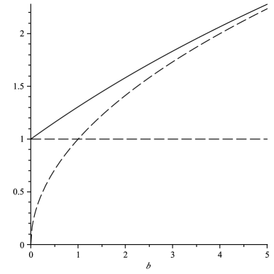
Figure 1. The eigenvalue $\hat{\lambda}_{b,\pi}$ for Weber’s equation $y^{\prime\prime}+(\lambda-bs^{2})y=0$, $y(\pm\pi/2)=0$ [solid curve]; shown also are the lower bounds $\hat{\lambda}\geq 1$ and $\hat{\lambda}\geq\sqrt{b}$ [dashed curves].

We note that there is also a useful lower bound for $\hat{\lambda}_{b,\pi}$, which we can arrive at as follows: The inclusion of $[-D/2,D/2]$ in $\mathbb{R}$ implies $\hat{\lambda}_{1,D}\geq\lim_{d\to\infty}\hat{\lambda}_{1,d}=1$, with eigenfunction $u(s)=\mathrm{e}^{-s^{2}/2}$. Therefore we also have

$$\hat{\lambda}_{b,\pi}=\sqrt{b}\hat{\lambda}_{1,\pi b^{1/4}}\geq\sqrt{b}.$$

This translates to an estimate for the drift eigenvalue $\bar{\lambda}_{a,\pi}$ appearing in Theorem 1.1: We have $\bar{\lambda}_{a,\pi}=\frac{a}{2}+\hat{\lambda}_{a^{2}/4,\pi}$, giving the following Taylor expansion:

$$\bar{\lambda}_{a,\pi} =1+\frac{a}{2}+\left(\frac{\pi^{2}}{12}-\frac{1}{2}\right)\frac{a^{2}}{4}+\left(\frac{\pi^{4}}{720}-\frac{5\pi^{2}}{48}+\frac{7}{8}\right)\frac{a^{4}}{16}+\left(\frac{\pi^{6}}{30240}-\frac{\pi^{4}}{48}+\frac{31\pi^{2}}{32}-\frac{121}{16}\right)\frac{a^{6}}{64}$$

$$\quad\hbox{}+\left(\frac{\pi^{8}}{362880}-\frac{\pi^{6}}{270}+\frac{683\pi^{4}}{1280}-\frac{14573\pi^{2}}{768}+\frac{17771}{128}\right)\frac{a^{8}}{256}+O(a^{10}).$$

In particular the lower bound $\hat{\lambda}\geq 1$ translates to $\bar{\lambda}\geq 1+a/2$, and the lower bound $\hat{\lambda}\geq\sqrt{b}$ translates to $\bar{\lambda}\geq a/2+\sqrt{a^{2}/4}=a$. Finally, by scaling we obtain the following:

$$\bar{\lambda}_{a,D} =\frac{\pi^{2}}{D^{2}}+\frac{a}{2}+\left(\frac{\pi^{2}}{12}-\frac{1}{2}\right)\frac{D^{2}a^{2}}{4\pi^{2}}+\left(\frac{\pi^{4}}{720}-\frac{5\pi^{2}}{48}+\frac{7}{8}\right)\frac{D^{6}a^{4}}{16\pi^{6}}$$

$$\quad\hbox{}+\left(\frac{\pi^{6}}{30240}-\frac{\pi^{4}}{48}+\frac{31\pi^{2}}{32}-\frac{121}{16}\right)\frac{D^{10}a^{6}}{64\pi^{1}0}$$

$$\quad\hbox{}+\left(\frac{\pi^{8}}{362880}-\frac{\pi^{6}}{270}+\frac{683\pi^{4}}{1280}-\frac{14573\pi^{2}}{768}+\frac{17771}{128}\right)\frac{D^{14}a^{8}}{256\pi^{14}}$$

$$\quad\hbox{}+O(D^{18}a^{10})\quad\text{\rm as}\ D^{2}a\to 0.$$

An interesting consequence of the Taylor expansion (combined with the fact that the estimate $\tilde{\lambda}_{1}\geq\bar{\lambda}_{a,D}$ is sharp as proved in section 2) is the following:

Proposition 4.1.

The constant $a/2$ in the lower bound $\tilde{\lambda}_{1}\geq\frac{\pi^{2}}{D^{2}}+\frac{a}{2}$ is the largest possible.

This follows from the Taylor expansion for small values of $aD^{2}$.

We note that the sharp diameter bound (given by the value of $a$ where the dotted line $\lambda=2a$ intersects with the solid curve in Figure 2) is not dramatically different from the one given in Corollary 3.1 (where the dotted line intersects the dashed line $\lambda=1+a/2$). Since the eigenvalue estimate $\tilde{\lambda}_{1}\geq\bar{\lambda}_{a,D}$ appears from the examples in section 2 to be sharp only in situations which are far from gradient solitons, we expect that neither of these diameter bounds is close to the sharp lower diameter bound for a nontrivial gradient Ricci soliton.

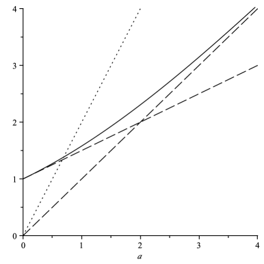
Figure 2. The eigenvalue $\bar{\lambda}_{a,\pi}$ for the drift Laplacian equation $y^{\prime\prime}-asy^{\prime}+\lambda y=0$, $y^{\prime}(\pm\pi/2)=0$ [solid curve]; shown also are the lower bounds $\bar{\lambda}\geq 1+\frac{a}{2}$ and $\bar{\lambda}\geq a$ [dashed lines], and the line $\bar{\lambda}=2a$ corresponding to non-Einstein gradient Ricci solitons [dotted line].