THE CARNEGIE-IRVINE GALAXY SURVEY. I. OVERVIEW AND ATLAS OF OPTICAL IMAGES

Abstract

The Carnegie-Irvine Galaxy Survey (CGS) is a long-term program to investigate the photometric and spectroscopic properties of a statistically complete sample of 605 bright ($B_{T}<12.9$ mag), southern ($\delta<0$^∘) galaxies using the facilities at Las Campanas Observatory. This paper, the first in a series, outlines the scientific motivation of CGS, defines the sample, and describes the technical aspects of the optical broadband (BVRI) imaging component of the survey, including details of the observing program, data reduction procedures, and calibration strategy. The overall quality of the images is quite high, in terms of resolution (median seeing $\sim 1$^′′), field of view (8$\farcm$9$\times$8$\farcm$9), and depth (median limiting surface brightness $\sim 27.5$, 26.9, 26.4, and 25.3 mag arcsec^-2 in the $B$, $V$, $R$, and $I$ bands, respectively). We prepare a digital image atlas showing several different renditions of the data, including three-color composites, star-cleaned images, stacked images to enhance faint features, structure maps to highlight small-scale features, and color index maps suitable for studying the spatial variation of stellar content and dust. In anticipation of upcoming science analyses, we tabulate an extensive set of global properties for the galaxy sample. These include optical isophotal and photometric parameters derived from CGS itself, as well as published information on multiwavelength (ultraviolet, $U$-band, near-infrared, far-infrared) photometry, internal kinematics (central stellar velocity dispersions, disk rotational velocities), environment (distance to nearest neighbor, tidal parameter, group or cluster membership), and H I content. The digital images and science-level data products will be made publicly accessible to the community.

1 Motivation

The structural components of a galaxy bear witness to the major episodes that have shaped them during its life cycle, and, as such, provide crucial fossil records of the physical processes operating in galaxy formation and evolution. Morphological clues have long guided our intuition about galaxy formation (Gott, 1977; Wyse et al., 1997). The two most conspicuous luminous components modulated along the Hubble sequence—the bulge and the disk—have been the main focal points of our modern concepts of how galaxies were assembled. The roughly spheroidal shape of elliptical galaxies and the bulges of spiral galaxies, along with the recognition of their generally evolved stellar population, signify rapid, dissipationless collapse at an early epoch. The $r^{1/4}$ profile (de Vaucouleurs, 1948) of ellipticals and classical bulges is often interpreted as a signature of viole0nt relaxation (van Albada, 1982) resulting from rapid assembly through major mergers. By contrast, the flattened configuration of an exponential disk (Freeman, 1970), along with their younger, more mixed stellar populations, suggests that more gradual, dissipative processes have been operating and are still ongoing today.

With the advent of modern, large-format detectors and the accompanying improvement in linearity, dynamic range, and image resolution, our view of galaxy morphology has grown steadily more elaborate, to the point that, in many instances, the classical picture of a bulge plus disk no longer suffices to describe the complex details seen in state-of-the-art galaxy images. While an $r^{1/4}$ law still provides a good first-order approximation to the overall light distribution of many elliptical galaxies, at least in images taken with typical ground-based resolutions, the situation is considerably more complicated for the bulges of disk galaxies. The central light distribution of not only spirals, but also S0s, shows a variety of shapes (e.g., Andredakis & Sanders, 1994; Courteau et al., 1996; de Jong, 1996; MacArthur et al., 2003; Laurikainen et al., 2005; Graham & Worley, 2008; Gadotti, 2009), which are often well represented by a Sérsic (1968) $r^{1/n}$ profile, with $n$ ranging from 1 (pure exponential) to 4 (standard de Vaucouleurs value). Imaging with the Hubble Space Telescope reveals an even greater degree of structural heterogeneity, including nuclear disks, nuclear spirals and rings, central nuclei and star clusters, and intricate dust lanes (e.g., Carollo et al., 1997; Böker et al., 2002; Seigar et al., 2002).

This rich variety of kinematically cold structures in the central regions of galaxies compels us to reevaluate the very definition of a “bulge.” Evidently many bulges are not the old, dead, fully established systems we once thought. Instead, they appear to have experienced a much more gradual, protracted history of formation in which secular evolutionary processes have been—and still are—at work. While most of the recent attention has focused on the phenomenon of “pseudobulges” (Kormendy & Kennicutt 2004, and references therein), there has also been a growing appreciation that even the classical bulges may have experienced a rather dynamic evolutionary history. Apart from the prevalence of features such as kinematically distinct or counterrotating cores, which are indicative of discrete accretion events (e.g., Forbes et al., 1995), many early-type galaxies contain nuclear gaseous disks and dust lanes (e.g., van Dokkum & Franx, 1995; Tran et al., 2001) and central stellar disks (e.g., Rix & White, 1992; Ledo et al., 2010), concrete reminders that these are continually evolving systems. In addition, a large fraction of disk galaxies ($\sim 30$%; Lütticke et al., 2000), including S0s (Aguerri et al., 2005), possess boxy or peanut-shaped bulges, which are believed to be not actual bulges at all but edge-on bars (e.g., Bureau & Freeman, 1999; Athanassoula, 2005; Kormendy & Barentine, 2010). This confounds our usual notion of what a bulge is, even in galaxies that are traditionally viewed as bulge-dominated.

The bulge does not live in isolation but is intimately linked with an extended disk, whose prominence relative to the bulge varies along the Hubble sequence. While to first order the disk can be approximated by a single exponential profile, which arises as a natural consequence of viscous dissipation (e.g., Lin & Pringle 1987), in detail it, too, exhibits a plethora of morphologically distinct features that may provide insights into more global formation processes. Pronounced departures occur at both small and large radii. At small radii, typically over scales where the bulge begins to dominate, some disks exhibit a downturn compared to the inner extrapolation of the outer exponential profile; Freeman (1970) called these “Type II” profiles. The central regions of late-type spirals, on the other hand, often show excesses above the outer extrapolated disk (Böker et al. 2003). On large scales, van der Kruit (1979) first noticed that the disks of some spiral galaxies have a sharply truncated outer edge, as opposed to those that maintain a single exponential profile that merges smoothly with the sky background. By contrast, there is a growing population of disks that shows the opposite effect—an upturn rather than a downturn—at large radii (Erwin et al. 2005). Still others possess what appears to be a distinct, highly extended secondary disk of very low surface brightness (Thilker et al. 2005; Barth 2007). The physical origin of these secondary outer-disk structures is not known, but a very intriguing possibility is that they might trace material accumulated from a recent episode of “cold accretion.” According to numerical simulations of cosmological structure formation (Murali et al. 2002), nearly pristine, primordial gas should be constantly raining down on galactic disks as it condenses and cools from the hot halo, providing the raw material for continued disk building.

Lastly, non-axisymmetric perturbations in the disk play a primary role in transferring angular momentum, thereby accelerating secular evolution by redistributing the gas, and even the stars (e.g., Friedli & Benz 1993; Athanassoula 2003). There are three main sources of non-axisymmetric perturbations: bars and barlike oval structures, spiral arms, and large-scale tidal distortions. For example, the phenomenon of “lopsidedness,” which may be a manifestation of minor mergers, subtle tidal interactions, or cold gas accretion (e.g., Zaritsky & Rix 1997; Levine & Sparke 1998; Bournaud et al. 2005), would manifest itself as an $m=1$ Fourier mode in azimuthal shape (e.g., Peng et al. 2010).

The phenomena outlined above have all been investigated in the past to varying degrees. Most previous studies have been quite restrictive, in terms of sample size, selection criteria, or wavelength coverage, often fine-tuned to address a narrow set of science goals. Notable examples of early CCD-based surveys include those of Kormendy (1985), Lauer (1985), and Schombert (1986) on early-type galaxies, and those of Kent (1985), Courteau (1996), and de Jong (1996) on spiral galaxies. More diverse samples exist, but they are often targeted to probe specific environments (e.g., the field: Jansen et al. 2000; nearby clusters: Gavazzi et al. 2003). Prior to the advent of modern all-sky surveys, two general-purpose samples of nearby galaxies have been widely used. Frei et al. (1996) assembled optical images for 113 bright ($B_{T}$ $\mathrel{\hbox{\hbox to0.0pt{\hbox{\lower 4.0pt\hbox{$\sim$}}\hss}\hbox{$<$}}}$ 12.5 mag) galaxies spanning a wide range of Hubble types; although no rigorous selection criteria were applied, this catalog has been extensively adopted for a variety of studies because the authors removed foreground stars from the images (Frei, 1996) and released the digital atlas to the public. The Ohio State University Bright Spiral Galaxy Survey (OSUBSGS; Eskridge et al. 2002) enforced more rigorous selection criteria to define a set of 205 galaxies and expanded the photometric coverage to the near-infrared (NIR). The lack of early-types in OSUBSGS compelled subsequent attempts to extend the sample to include S0 systems, but only in the NIR (Laurikainen et al. 2005; Buta et al. 2006). Despite the utility of the Frei and OSUBSGS samples, they had limitations in terms of image quality and filter set. Both surveys employed imager-telescope systems that resulted in rather coarse pixel scales, $\sim$1$\farcs$2-1$\farcs$4 pixel^-1 in the case of Frei, and $\sim$0$\farcs$4-0$\farcs$7 pixel^-1 in the case of OSUBSGS. The image quality was especially heterogeneous for OSUBSGS, having been conducted using multiple detectors on six different telescopes.

The considerations outlined above motivated us to initiate the

$B$-band luminosity function for the CGS sample, computed with the $1/V_{\rm max}$ method of Schmidt (1968). Superposed for comparison is the $r$-band luminosity function of $z\approx 0.1$ galaxies selected from SDSS (Blanton et al. 2003), shifted by $B-r=0.67$ mag, the average color of an Sbc spiral (Fukugita et al. 1995), which is roughly the median Hubble type of the CGS sample. The overall agreement indicates that CGS provides an unbiased representation of the nearby galaxy population.

Figure 1: Basic properties of the CGS sample. Distribution of (a) total apparent $B$ magnitude, (b) distances, (c) absolute $B$ magnitude, corrected for Galactic extinction, and (d) $B$-band isophotal diameter at $\mu_{B}$ = 25 mag arcsec^-2.

Carnegie-Irvine Galaxy Survey (CGS), a long-term program to investigate the photometric and spectroscopic properties of a large sample of nearby galaxies, using the facilities at Las Campanas Observatory. Given the availability of large databases such the Sloan Digital Sky Survey (SDSS; York et al. 2000) or the Two Micron All-Sky Survey (2MASS; Skrutskie et al. 2006), it might seem counterintuitive that a new galaxy imaging survey is necessary. As described below, our optical images have significantly better resolution than SDSS images. Moreover, only 9% (56/605) of the galaxies in CGS overlap with the SDSS footprint: SDSS does not cover the vast majority of bright southern galaxies. As the images are a vital precursor to the spectroscopic component of the survey that we are planning to conduct, we have undertaken a uniform imaging program for CGS.

This paper gives a general overview of the optical imaging component of CGS and summarizes a suite of ancillary data that will be used in subsequent analyses of the survey. A companion paper by Li et al. (2011; hereafter Paper II) describes the analysis of the surface brightness profiles and isophotal parameters of the sample. Future papers will present the NIR imaging, detailed structural decompositions of the galaxies, and scientific applications thereof.

2 Sample

2.1 Survey Definition

To fully capture the wealth and range of the morphological properties of the local galaxy population, to maximize signal-to-noise ratio (S/N) and spatial resolution, and to ensure statistical completeness, we target a large, well-defined sample of the brightest objects optimally placed for Carnegie’s facilities at Las Campanas Observatory. We impose no selection according to galaxy morphology, size, or environment. The sample, consisting of 605 objects, is formally defined by $B_{T}\leq 12.9$ mag and $\delta<0$^∘. The completeness level of bright galaxies to this magnitude limit is essentially 100% (Paturel et al. 2003), yielding a sample roughly comparable in size to that of the Palomar survey of northern galaxies (Ho et al. 1995, 1997a), which is desirable for future comparisons between the two hemispheres. In practice, we select objects from the Third Reference Catalogue of Bright Galaxies (RC3; de Vaucouleurs et al. 1991),

Figure 2: Distribution of morphological types in CGS. The bottom axis gives the type index $T$, and the corresponding Hubble types are shown on the top axis (E: $T=-5$ to $-4$; S0: $-3$ to $-1$; S0/a: 0; Sa: 1; Sb: 3; Sc: 5; Sd: 7; Sm: 9; Im: 10). Barred (B and AB) and unbarred galaxies are shown in filled and open histograms, respectively.

with the aid of the online database HyperLeda (Paturel et al. 2003).

CGS provides a fair, statistically unbiased representation of the local galaxy population over the absolute magnitude range $-16$ $\mathrel{\hbox{\hbox to0.0pt{\hbox{\lower 4.0pt\hbox{$\sim$}}\hss}\hbox{$<$}}}$ $M_{B_{T}}$ $\mathrel{\hbox{\hbox to0.0pt{\hbox{\lower 4.0pt\hbox{$\sim$}}\hss}\hbox{$<$}}}$ $-23$. This is illustrated in Figure 1, which shows the $B$-band luminosity function calculated using the $1/V_{\rm max}$ method of Schmidt (1968), compared with the $r$-band luminosity function of $z\approx 0.1$ galaxies derived from the SDSS by Blanton et al. (2003). In making this comparison, we assume a typical galaxy color for Sbc galaxies ($B-r=0.67$ mag; Fukugita et al. 1995), which is approximately the median morphological type of CGS, and a Hubble constant of $H_{0}=73$ km s^-1 Mpc^-1. The two functions agree quite well, both in shape and in normalization. The relatively large fluctuations on the faint end of the luminosity function reflect the density inhomogeneities in the local volume.

Table 1 and Figure 2 summarize some of the basic parameters of the sample. Given the bright magnitude limit of the survey (Figure 2(a)), it is not surprising that most of the galaxies are quite nearby (median $D_{L}$ = 24.9 Mpc; Figure 2(b)), luminous (median $M_{B_{T}}=-20.2$ mag, corrected for Galactic extinction; Figure 2(c)), and angularly large (median $B$-band isophotal diameter $D_{25}$ = 3$\farcm$3; Figure 2(d)).

The sample spans the full range of Hubble types in the nearby universe (Figure 3), comprising 17% ellipticals, 18% S0 and S0/a, 64% spirals, and 1% irregulars. A handful of well-known interacting systems (e.g., the “Antennae,” Centaurus A, NGC 2207) are included, but the vast majority of the sample have relatively undisturbed morphologies, although the RC3 classifications designate $\sim$16% of the sample as “peculiar” in some form. As with the Palomar sample (Ho et al. 1997b), roughly 2/3 of the disk (S0 and spiral) galaxies are barred according to the classifications in the RC3, with the breakdown into strongly barred (SB) and weakly barred (SAB) being 37% and 29%, respectively. Approximately 10% have an outer ring or pseudoring (Buta & Crocker 1991).

In addition to the parent sample of 605 galaxies, Table 1 also lists 11 sources that were observed early in the survey prior to it being fully defined, but that now formally do not meet the magnitude limit of the survey. We include these extra objects for completeness, but they will be omitted from future statistical analyses.

3 Observations

All the images for CGS were taken with the du Pont 2.5 m telescope, during the period 2003 February to 2006 June, spread over 69 nights and nine observing runs. Table 2 gives a log of the observations. For the optical component of the survey, we employed the 2048$\times$2048 Tek#5 CCD camera, which has a scale of 0$\farcs$259 pixel^-1, sufficient to Nyquist sample the sub-arcsecond seeing often achieved with the du Pont telescope. The field of view of 8$\farcm$9$\times$8$\farcm$9 is large enough to enclose most of the galaxies, which have a median isophotal diameter of $D_{25}$ = 3$\farcm$3 at a surface brightness level of $\mu_{B}=25$ mag arcsec^-2 (Figure 2(d)), while still allowing adequate room for sky measurement. As discussed in Section 4.4, background subtraction is a key factor that limits the accuracy of structural decomposition and detection of faint outer features. A subset of the larger galaxies were reimaged at lower resolution with the Wide-field CCD, which has a field of view of 26^′$\times$26^′ and a scale of 0$\farcs$77 pixel^-1; these data will be presented elsewhere.

Each galaxy was imaged in the Johnson $B$ and $V$ and Kron–Cousins $R$ and $I$ filters, typically for total integration times of 12, 6, 4, and 6 minutes, respectively, split into two equal-length exposures to facilitate rejection of cosmic rays and to mitigate saturation. The centers of some galaxies were still saturated even with these integration times, and we took short ($\sim 10-60$ s) exposures to obtain unsaturated images of the core. In total, over 6000 science images were collected. Standard calibration frames for optical CCD imaging were taken, including a series of bias frames, dark frames, and flat fields from the illuminated dome and the twilight sky. During clear nights, we observed a number of photometric standard star fields from Landol92, covering stars with a range of colors and tracking over a range of airmasses.

A significant fraction of the sample was also imaged in the $K_{s}$ (2.2 $\mu$m) band using the Wide-field Infrared Camera, a cryogenically cooled mosaic of four 1024$\times$1024 arrays that delivers 13^′$\times$13^′ images with excellent image quality (scale 0$\farcs$2 pixel^-1). These observations will be presented elsewhere.

4 Data Reductions

4.1 Basic Processing

The initial processing follows standard steps for CCD data reduction within the IRAF environment, using tasks within ccdproc, which include trimming, overscan correction, bias subtraction, and flat fielding. Dark current subtraction is unnecessary. We took dark frames with integration times comparable to those of the longest science exposures, but the dark current always turns out to be negligible. For each night of each observing run, we generate a master bias frame by averaging a large number (typically $\sim 20$) of individual bias frames. Similarly, we create a master flat-field frame with high S/N by combining a series (typically $\sim 6-10$ per filter) of domeflats and twiflats. Through experimentation, we found that the twiflats produce more uniform illumination than the domeflats for the $B$ and $V$ images, whereas the domeflats are more effective for the $R$ and $I$ images. A small fraction of the flats contained dust specks that introduced “doughnut” features into the flattened frames; roughly $\sim 4$% of the science images were affected by this. The flattened $I$-band images contain subtle, residual fringe patterns with amplitudes (peak to trough) at the level of $\sim$1%–2%. We remove these by subtracting an optimally scaled fringe frame with a mean zero background, which was constructed by median combining a total of 36 sky images collected over many observing runs. The fringe pattern proved to be remarkably stable throughout the course of the survey. Apart from a couple of partially dead columns near the center of the chip, the Tek#5 CCD is relatively clean cosmetically. We generate a mask for these and other less conspicuous defective regions, and use it for local interpolation to correct the bad pixels. Finally, we use an IDL version of van Dokkum’s (2001) L.A.Cosmic routine to correct the pixels affected by cosmic ray hits and satellite trails; any remaining imperfections were further edited manually.

Next, we shift and align the flattened, cleaned images in each filter to a common reference frame defined by the $I$-band image, which generally has the sharpest seeing and is least affected by possible dust obscuration. Multiple images taken with the same filter were combined. We carefully examine the images for possible saturation near the core of the galaxy and replace any saturated pixels with their appropriately scaled counterparts from the short-exposure images. We determine the proper scale factor by comparing the background-subtracted, integrated counts of bright, isolated field stars that are unsaturated in both the long and short exposures. The affected regions are generally small, spanning a diameter of only $\sim 10$ pixels. As this is not significantly larger than the point-spread function (PSF), this procedure has a negligible impact on any of our subsequent scientific analysis. For convenience, we flip the images so that north points up and east to the left. Lastly, we use the Astrometry.net (Lang et al. 2010) software to solve for the World Coordinate System (WCS) coordinates of each image and store them in the FITS header.

4.2 Photometric Calibration

A little more than half of the CGS galaxies were observed under photometric conditions, as determined from observations of Landolt (1992) standard stars. We measure the photometry of the stars using a circular aperture with a fixed radius of 7^′′, to mimic as closely as possible Landolt’s measurements. We determine the local sky of each star from a 5 pixel wide annulus outside that aperture, using only sky pixels (i.e., avoiding any nearby neighboring stars). The median photometric errors (Table 2, Column 9) for the photometric nights are 0.08, 0.04, 0.03, and 0.04 mag for the $B$, $V$, $R$, and $I$ band, respectively. The images calibrated in this manner have the header keyword ZPT_LAN.

For the non-photometric observations, we adopt an indirect approach that allows us to obtain a less accurate, but still useful, photometric calibration. Our strategy is to bootstrap the instrumental magnitudes of the brighter stars within each CCD field to their corresponding photographic magnitudes as published in the second-generation Hubble Space Telescope Guide Star Catalog (GSC2.3; Lasker et al. 2008). We derive the transformation between the GSC photographic bandpasses and our standard BVRI magnitudes using the subset of field stars that were observed by us under photometric conditions. The GSC contains astrometry, photometry, and object classification for nearly a million objects. The photometry for the southern hemisphere is given primarily in three photographic bandpasses, $B_{J}$, $R_{F}$, and $I_{N}$. The typical photometric error for the stellar objects in the GSC, depending on the magnitude and passband, is 0.13–0.22 mag (Lasker et al. 2008).

Starting with the list of WCS coordinates extracted for the field stars in each CCD image, we use the Vizier server to query the GSC for objects classified therein as stellar (class = 0). We eliminate saturated objects and stars fainter than $B\approx 22$ mag. To properly compare our instrumental magnitudes with the GSC magnitudes, it is critical that we follow as closely as possible the methodology that the GSC used to derive their photometry. We cannot use conventional methods of stellar aperture photometry (e.g., using standard tasks in IRAF). As outlined in Lasker et al. (2008), the procedures used in the GSC for object detection, flux measurement, sky determination, and source deblending in the case of crowded fields (Beard & MacGillivray 1990) follow very closely those implemented in the SExtractor package (Bertin & Arnouts 1996). We therefore use SExtractor to measure the stars in our CGS images. We manually performed aperture photometry of a number of isolated stars to confirm that the SExtractor-based measurements are reliable, to better than 0.02 mag.

We intercalibrate the CGS and GSC photometric scales using data from a night with exceptional photometric stability, during which the open cluster M67 was observed. Our photometry for M67 agrees very well with that published by Montgomery et al. (1993), to better than 0.01 mag, for all filters. Using a set of $500-600$ field stars selected from the science images observed throughout the course of that night, we derive a set of transformation equations between the GSC photometric bandpasses ($B_{J}$, $R_{F}$, and $I_{N}$) and our standard bandpasses ($B$, $V$, $R$, and $I$). The fitting was done with the IDL function ladfit, which uses a robust least absolute deviation method and is not sensitive to outliers. The transformation equations and residual scatter ($\sigma$) (in magnitudes) for each filter are as follows:

$$B = B_{J}+0.2807-0.1365(B_{J}-R_{F})\quad\qquad\sigma=0.2088$$ (1)

$$B = B_{J}+0.1499+3.239\times 10^{-5}(B_{J}-I_{N})\quad\sigma=0.2490$$ (2)

$$B = 0.1489+1.0001B_{J}\ \ \ \ \ \ \qquad\qquad\qquad\sigma=0.2597$$ (3)

$$B = R_{F}+0.9700+0.8888(R_{F}-I_{N})\ \ \ \ \qquad\sigma=0.2982$$ (4)

$$B = 0.4508+1.0468R_{F}\ \ \ \ \ \qquad\qquad\qquad\sigma=0.3832$$ (5)

$$B = 0.8471+1.0488I_{N}\ \ \ \ \ \ \qquad\qquad\qquad\sigma=0.6058$$ (6)

$$V = B_{J}+0.1512-0.6625(B_{J}-R_{F})\qquad\quad\sigma=0.1140$$ (7)

$$V = R_{F}+0.4658+0.2279(R_{F}-I_{N})\qquad\quad\sigma=0.1721$$ (8)

$$V = B_{J}+0.0060-0.3982(B_{J}-I_{N})\ \qquad\quad\sigma=0.1760$$ (9)

$$V = 0.8077+0.9825R_{F}~{}\ \ \ \ \ \qquad\qquad\qquad\sigma=0.1828$$ (10)

$$V = 0.7665+0.9232B_{J}\ \ \ \ \ \ \qquad\qquad\qquad\sigma=0.2775$$ (11)

$$V = 0.0875+1.0499I_{N}~{}\ \ \ \ \ \ \qquad\qquad\qquad\sigma=0.3780$$ (12)

$$R = R_{F}+0.1380-0.2667(R_{F}-I_{N})\qquad\quad\sigma=0.0976$$ (13)

$$R = 1.2166+0.9286R_{F}\ \ \ \ \ \ \qquad\qquad\qquad\sigma=0.1121$$ (14)

$$R = I_{N}-0.0954+0.3353(B_{J}-I_{N})~{}\ \qquad\quad\sigma=0.1257$$ (15)

$$R = R_{F}-0.0208+0.0551(B_{J}-R_{F})\qquad\quad\sigma=0.1264$$ (16)

$$R = -0.2960+1.0441I_{N}~{}~{}\ \ \ \ \qquad\qquad\qquad\sigma=0.2301$$ (17)

$$R = 1.5288+0.8546B_{J}\ \ \ \ \ \ \ \qquad\qquad\qquad\sigma=0.3509$$ (18)

$$I = I_{N}-0.1119+0.0931(R_{F}-I_{N})\ \qquad\quad\sigma=0.0924$$ (19)

$$I = I_{N}-0.0709+0.0152(B_{J}-I_{N})~{}\ \qquad\quad\sigma=0.1073$$ (20)

$$I = -0.1713+1.0079I_{N}\ \ \ \ \ \qquad\qquad\qquad\sigma=0.1164$$ (21)

$$I = R_{F}-0.2323-0.2276(B_{J}-R_{F})\qquad\quad\sigma=0.2000$$ (22)

$$I = 1.6690+0.8728R_{F}\ \ \ \ \ \ \qquad\qquad\qquad\sigma=0.2244$$ (23)

$$I = 2.5445+0.7739B_{J}~{}~{}\ \ \ \ \ \qquad\qquad\qquad\sigma=0.4543$$ (24)

For any given CCD frame, the calibration equation we choose depends on which GSC bandpasses are available for that particular field; all else being equal, we select the transformation equation that has the smallest scatter. The images calibrated in this manner have the keyword ZPT_GSC in the header. The median photometric uncertainty (Table 2, Column 9) of the GSC-based magnitudes, which is dominated by the error in the above fitting equations, is 0.21, 0.11, 0.098, and 0.092 mag for the $B$, $V$, $R$, and $I$ band, respectively.

4.3 Masks and Point-spread Function

Many aspects of the survey require that we exclude signal contributed by unrelated objects, such as foreground stars and background galaxies. This is achieved by creating a mask that properly identifies the affected pixels. We begin by running SExtractor to identify all the objects in the image and classify them into stellar and nonstellar sources based on their compactness relative to the seeing. Through experimentation, we find that a “class parameter” larger than 0.3 effectively isolates the stars from the resolved objects. During this initial step, we deliberately set the contrast parameter to a moderate value (we set the threshold to be 3 $\sigma$ above the background) so that galaxies with substantial internal structure (e.g., spirals and irregulars) do not get broken up into multiple pieces. This, in turn, implies that SExtractor will miss fainter stars that might be superposed on the main body of the central galaxy. We carefully examine each image visually and manually add additional objects to the segmentation image if necessary. Next, two segmentation images are created, one to isolate the unsaturated stellar objects and the other the nonstellar objects, which include background galaxies and saturated stars (including their bleed trails, if present). Because we set the contrast parameter to a conservative level, the segmentation images identify only the bright core regions of the objects to be masked and often miss their fainter outer halos, which can be substantial, especially for bright stars in the $I$ band. To account for these regions, we need to “grow” the segmentation image of each object. From trial and error, we find that a growth of 8 pixels in radius is optimal for the stellar objects. For the nonstellar objects, we distinguish between two regimes. A growth radius of 5 pixels is sufficient for bright bleed trails. For the fainter, more extended halos, we find that the growth radius can be approximated by $R={\rm min}[15,1.5\ \sqrt{N/\pi}]$, where $N$ is the number of pixels contained in the original segmentation image. Lastly, we stack together the masks of each individual filter to create a master mask for each galaxy, which is then used in all subsequent analysis, to ensure that all filters reference the same set of pixels.

We use the IRAF task psf within the daophot package and the bright, unsaturated stars identified by SExtractor in the previous step to build an empirical PSF for each image. The PSF image is a key ingredient in much of our analysis, including generation of the structure maps (Section 5) and bulge-to-disk decomposition (S. Huang et al., in preparation).

4.4 Image Quality

The bulk of the CGS observations have fairly good image quality. The seeing, as estimated from the full width at half-maximum (FWHM) of the radial profiles of bright, unsaturated stars, ranges between $\sim$0$\farcs$5, the limit we can measure given

Distribution of seeing values for the CGS images, shown separately for each of the four filters. The legend gives the median and interquartile (IQR) range of each histogram.

the pixel scale of our detector, to $\sim 2$^′′, with a median value of 1$\farcs$17, 1$\farcs$11, 1$\farcs$01, and 0$\farcs$96 in the $B$, $V$, $R$, and $I$ band, respectively (Figure 4). The main factors that limit the surface brightness sensitivity of the images stem from residual errors in flat fielding and uncertainties in sky determination. We have discovered that large variations in the ambient temperature and humidity throughout the night can occasionally produce water condensation on the surfaces of some of the filters. This effect imprints large-scale flat-fielding errors at the level of $\sim 1\%$. Background gradients of a roughly similar magnitude are sometimes induced by scattered light from very bright stars, either within or just outside the science frame. These anomalies can be mitigated by fitting a two-dimensional polynomial function to the background pixels (Noordermeer & van der Hulst 2007; Barazza et al. 2008; Erwin et al. 2008). A second-order polynomial function usually suffices, but in some cases the order of the polynomial may need to be as high as 5. The fitting regions are source-free pixels far from the main galaxy, selected from the image after convolving it with a Gaussian with FWHM $\approx$ 4^′′–5^′′ to accentuate low-spatial frequency features. This correction typically improves the flatness of the images by about a factor of 2, from $\sim 1\%$ to $\sim 0.6\%$. Once the background is flat, determining its value is relatively straightforward because most of the survey galaxies have sizes (median $D_{25}$ = 3$\farcm$3; Figure 2(d)) that fit comfortably within the field of view of the detector (8$\farcm$9$\times$8$\farcm$9). The larger galaxies ($D_{25}$ $\mathrel{\hbox{\hbox to0.0pt{\hbox{\lower 4.0pt\hbox{$\sim$}}\hss}\hbox{$>$}}}$ 5^′–6^′; $\sim$15% of the sample), however, pose a challenge, and we are forced to implement an indirect, less reliable strategy for sky subtraction (Paper II). The surface brightness depth of the images (Table 2, Column 10), which we define to be the isophotal intensity that is 1 $\sigma$ above the sky rms, has a median value of $\mu\approx 27.5$, 26.9, 26.4, and 25.3 mag arcsec^-2 in the $B$, $V$, $R$, and $I$ bands, respectively.

5 Images

In anticipation of future applications of the survey, we prepare several different renditions of the digital images, which are described below. The full image atlas for the 605 galaxies in CGS (including the 11 “extras”) is given in the Appendix, as Figures 7.1–7.616, as well as on the project Web site http://cgs.obs.carnegiescience.edu.

• Color composites. We generate three-color composites from the $B$, $V$, and $I$ images by applying an arcsinh stretch (Lupton et al. 2004) to each of these bands and then using them to populate the blue, green, and red channels of the color image. The arcsinh stretch is particularly effective in viewing a broad dynamic range of structure.

• Star-cleaned images. A variety of scientific applications can benefit from galaxy images that are free from contamination by foreground stars and background galaxies. An example would be using nearby galaxies as templates to simulate higher redshift observations. Our procedure to “clean” the galaxy images begins by using the object mask created from SExtractor (Section 4.3) to identify all the stellar and nonstellar objects that need to be removed. For every given image, we use the task allstar to fit the empirical PSF appropriate for that image to all the unsaturated stars and subtract them. As the PSF varies slightly across the field, the subtraction is imperfect and small residuals often remain around the positions of bright stars. To improve the cosmetic appearance of the images, we devised the following scheme to locally interpolate over the residuals. For every star, we fit a two-dimensional function to a 5 pixel wide annular region immediately exterior to its grown segmentation image. We find the exponential function to be quite effective—more so than a tilted plane or a second-order polynomial—as it has enough flexibility to handle steep local gradients often encountered for complex galaxy backgrounds. Each pixel within the segmentation image is then compared with the best-fitting function value at that position. If they differ by more than 2 times the mean value of the differences between the pixels in the background annulus and the best-fit pixel values there, it gets replaced with the best-fit pixel value. We add noise to the replaced pixel, drawn randomly, using the IDL function randomu, from the distribution of residuals calculated from the background annulus. The nonstellar objects are treated in exactly the same manner, except that for these PSF subtraction is unnecessary.

  The above procedure works very effectively most of the time, as illustrated for a couple of examples in the top and middle panels of Figure 5. It performs less successfully for heavily saturated bright stars that are directly superposed on the science target, especially those with prominent bleed trails, as shown in the example in the bottom panel of the figure. Under these circumstances, almost any local interpolation scheme will produce a highly compromised result. For these situations, we extract, in conjunction with the SExtractor object mask, the surface brightness profile and isophotal parameters of the galaxy using the IRAF task ellipse, as described in Paper II. These isophotes then serve as the basis for building a smooth representation of the intrinsic light distribution of the galaxy using the task bmodel, which, when combined with the original object mask, gives a reasonably realistic estimate of the underlying galaxy light affected by the masked regions. The corrupted regions were replaced with the corresponding pixel values from the model image, and Poisson noise is added. If a saturated star falls near the center of the galaxy, we

  

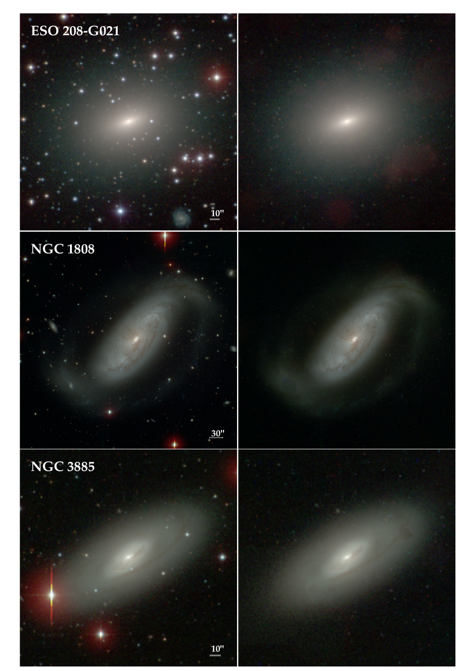
  Figure 3: Examples to illustrate our technique to clean the images of foreground stars and background galaxies. We use the three-band composite for both the original and star-cleaned images, displayed using an arcsinh stretch.

  

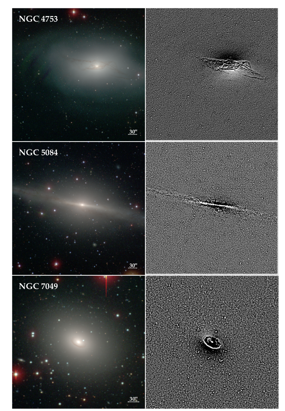
  Figure 4: Examples to illustrate the ability of the structure maps to bring out fine structure. The left panel shows the BVI color composite on an arcsinh stretch, and the right panel shows the structure map of the star-cleaned $B$-band image on a linear stretch.

  first attempt to replace it with an unsaturated version using the short exposure, following the same procedure for treating saturated cores. We apply this alternative procedure only to those regions wherein our local interpolation scheme fails to do a good job.

• Stacked images. In an effort to improve the S/N and to enhance the visibility of features with low surface brightness, we create a stacked image for each galaxy by combining the processed individual images from each of the four filters. We did not match the seeing among the images, as such a process, which involves smoothing, would alter the noise properties of the images; this is not critical for the stacked images because we are mainly interested in emphasizing diffuse features, which are insensitive to the seeing. This technique has been used to detect faint structures in both nearby (van Dokkum 2005) and distant (Gawiser et al. 2006) galaxies. As in Gawiser006, their Appendix A), we weight the data by S/N² to optimize for surface brightness, after first normalizing all the images so that 1 count corresponds to AB = 30 mag. We follow Frei & Gunn (1994) to convert our BVRI magnitudes to the AB system. To compute the weights, we determine the signal from the mean flux of 10–20 bright stars in common among the different images, and the noise from the standard deviation of the sky pixels.

• Structure maps. There are a variety of ways to spatially filter an image to emphasize structures on different scales. The structure map technique developed by Pogge & Martini (2002) is particularly effective in enhancing spatial variations on the smallest resolvable scales, namely that of the PSF. For every image in the survey, we calculate the structure map $S$, defined as

  $$S=\left({{I}\over{I\otimes P}}\right)\otimes P^{\phantom{.}t},$$ (25)

  where $I$ is the star-cleaned image taken in a particular filter, $P$ is the corresponding PSF image (see Section 4.3), $P^{\phantom{.}t}$ is the transpose of the PSF, such that $P^{\phantom{.}t}(x,y)=P(-x,-y)$, and the operator $\otimes$ denotes convolution. Figure 6 illustrates the utility of the structure map in highlighting small-scale spatial variations in an image.

• Color index maps. Our multi-filter data set allows us to study two-dimensional distributions of color, which trace spatial variations of dust and stellar content. A color index map is generated simply by dividing two registered images taken in the relevant filters, after sky subtraction and matching the two images to a common PSF. We convolve the image with the better seeing with a two-dimensional Gaussian function whose width is the quadrature difference of the two seeing values. We create the following set of color index maps: $B-V$, $B-R$, $B-I$, $V-I$, and $R-I$.

6 Tabulated Data

6.1 Isophotal and Photometric Parameters Derived from CGS

Paper II presents the brightness profiles and isophotal parameters of the survey. A number of basic, but nonetheless useful, global parameters for the galaxies can be derived from those data. We summarize them here. The advantage of our measurements is that they are derived in a uniform, self-consistent manner.

Table 3 lists several size measurements derived from the $B$-band images. We choose this bandpass because it closely matches most published measurements in the literature. The quantities $R_{20}$, $R_{50}$, and $R_{80}$ are the radii enclosing, respectively, 20%, 50%, and 80% of the total flux, which is calculated from integrating the surface brightness profile generated using the IRAF task ellipse (see Paper II). We define the concentration parameter as $C=R_{80}/R_{20}$. The isophotal diameters, measured at a surface brightness level of $\mu_{B}=25.0$ and 26.5 mag arcsec^-2, are given as $D_{25}$ and $D_{26.5}$, while $D^{c}_{25}$ and $D^{c}_{26.5}$ are the corresponding values corrected for Galactic extinction ($A_{B}$ in Table 1, taken from Schlegel et al. (1998) and inclination effect, following the prescription of Bottinelli et al. (1995). For galaxies with morphological types $T>-3.5$, we derive the inclination angle of the disk, $i$, using Hubble’s (1926) formula

$${\rm cos}^{2}i={{(1-e)^{2}-q_{0}^{2}}\over{1-q_{0}^{2}}},$$ (26)

which makes use of the apparent ellipticity ($e$) of the outer regions of the disk. The intrinsic flattening of the disk depends mildly on morphological type (Paturel et al. 1997), but for simplicity we adopt a constant value of $q_{0}=0.2$ (Noordermeer & van der Hulst 2007). The position angle (PA) of the photometric major axis, east of north, is also given. Unlike the other parameters in this table, both $e$ and PA are measured from the $I$-band image rather than from the $B$-band image in order to minimize possible distortions from dust or patchy regions of star formation. These quantities are determined from the outer regions of the galaxy—far enough to be insensitive to the bulge and bar but not so much so to be affected by lopsidedness in the outer disk or imperfect flat fielding—where they usually converge to a constant value. The listed uncertainties represent the standard deviation about the mean. In cases where $e$ and PA do not converge, we estimate them visually from the best-fitting isophotes at large radii. Lastly, we tabulate $\Sigma$, the sum of the rms fluctuations in the structure map of the $B$-band image, which gives a useful relative measure of the degree of high-spatial frequency fluctuations present in the image.

Table 4 presents BVRI integrated magnitudes derived from the star-cleaned images (Section 5). Two measurements are made: $m_{25}$ pertains to the total apparent magnitude within the $\mu=25$ mag arcsec^-2 isophote, whereas $m_{\rm tot}$ derives from the total flux within the largest isophote fitted to the image. The main uncertainty of the magnitudes comes from the uncertainty of the photometry zero point, with little contribution from sky error or Poisson noise. For convenience, we provide the absolute magnitudes in the $B$ band, corrected for Galactic extinction as given in Table 1 and adopting the luminosity distances therein.

Table 5 lists $\mu_{e}$, the surface brightness measured at the effective or half-light radius $R_{50}$, for each of the four filters.

6.2 Photometric Data from the Literature

Table 6 assembles multiwavelength photometric data from several large galaxy catalogs. The listed values represent total integrated fluxes for the entire galaxy. Instead of collecting data from any available literature source, we restrict our selection to only a few well-documented, homogeneous compilations. For the ultraviolet, we select FUV (1350–1750 Å) and NUV (1750–2800 Å) measurements principally from the Galaxy Evolution Explorer (GALEX) atlases of Buat et al. (2007), Dale et al. (2007), and Gil de Paz et al. (2007). At present, only $\sim 16\%$ of our sample has published GALEX data, although the situation will soon improve substantially with the recent completion of the All-Sky Imaging Survey. To extend the optical coverage blueward of the $B$ band, we searched HyperLeda for $U$-band (3500 Å) photometry, which is available for 63% of the sample. The most complete coverage is in the near-infrared ($J$, $H$, and $K_{s}$ bands) and far-infrared (12, 25, 60, and 100 $\mu$m); $\sim$95% of the galaxies are included in the Two Micron All-Sky Survey (2MASS; Skrutskie et al. 2006) and in the source catalogs of the Infrared Astronomical Satellite (IRAS). Because our galaxies are angularly large, care is taken to choose photometry derived from studies that properly treat extended sources (Jarrett et al. 2003; Sanders et al. 2003). In addition to the flux densities in the individual IRAS bands, we also give the parameter FIR, defined as 1.26$\times$10^-14 (2.58$S_{60}\,+\,S_{100}$) W m^-2, which approximates well the total flux between 42.5 and 122.5 $\mu$m (Helou et al. 1988; Rice et al. 1988). To date, $\sim 70$% (406/605) of our sample have been observed at 3.6 and 4.5 $\mu$m using the Infrared Array Camera on Spitzer. Roughly 60% of our sample overlaps with the Spitzer Survey of Stellar Structure in Galaxies (S⁴G; Sheth et al. 2010). We intend to incorporate these mid-infrared data into CGS in the future.

6.3 Kinematics, Environment, and Gas Content

Three categories of data are included in Table 7. We assemble from HyperLeda information on the internal kinematics of the galaxies, namely the apparent maximum rotation velocity of the gas ($V_{\rm max}$), the maximum rotation velocity corrected for inclination ($V_{\rm rot}$), and the central stellar velocity dispersion ($\sigma_{\star}$).

Next, we provide three environmental indicators. Using the facilities in the NASA/IPAC Extragalactic Database (NED), we search for candidate neighbors within a radius of 750 kpc. (NED restricts environmental searches to a maximum radius of 600^′, and, for a handful of objects, this corresponds to less than 750 kpc.) We calculate the projected angular separation, $\Delta\theta$, in units of the diameter $D_{25}$ (Table 3), to the nearest neighboring galaxy having an apparent magnitude brighter than $B_{T}\,+\,1.5$ mag and a systemic velocity within $\upsilon_{h}\,\pm\,500$ km s^-1. These criteria select sizable objects, with luminosity ratios of at least 4:1, which are likely to be physically associated companions. When no neighbor that satisfies the above criteria is found, $\Delta\theta$ is given as a lower limit. Following Bournaud et al. (2005), we also calculate the tidal parameter

$$t_{p}\equiv\log\left\{\sum_{i}\frac{M_{i}}{M_{0}}\left(\frac{R_{0}}{D_{i}}\right)^{3}\right\},$$ (27)

where $M_{0}$ and $R_{0}$ are the mass and size of the galaxy in question, $M_{i}$ and $D_{i}$ are the mass and projected separation of neighbor $i$, and the summation is performed over all neighbors with systemic velocities within $\upsilon_{h}\,\pm\,500$ km s^-1 in a region with a radius of 750 kpc. For simplicity, we assume that all galaxies have the same mass-to-light ratio and adopt the Johnson $B$ band as the reference filter. To the extent possible, we convert photometry listed in other bandpasses to the $B$ band, assuming colors typical of an Sbc galaxy (Fukugita et al. 1995; Peletier & de Grijs 1998). An uncertainty of up to 0.3 mag, which encompasses the extreme range of plausible $K$ corrections for different Hubble types, introduces an error of 0.12 dex in $t_{p}$. We set $R_{0}=0.5D_{25}$. Lastly, we indicate whether the galaxy belongs to the field or to a known galaxy group or cluster. The main cluster in the southern sky pertinent to CGS is Fornax, and we draw our membership identifications from Ferguson (1989) and Ferguson & Sandage (1990). Most of the group assignments come from the 2MASS-based group catalog of Crook et al. (2007).

The last two columns of Table 7 summarize the neutral hydrogen content. The H I  (21 cm) flux, in magnitude units, is defined such that $m_{21}^{c}=-2.5\log f+17.40$, where the integrated line flux $f$ is in units of Jy km s^-1. We adopted the correction for self-absorption as given in HyperLeda. In the optically thin limit, the H I mass is given by

$$M_{{\rm H~{}{I}}}=2.36\times 10^{5}\ D_{L}^{2}\ f\,\,\,\,M_{\odot},$$ (28)

where $D_{L}$ is the luminosity distance expressed in Mpc (Roberts 1962). We list the H I mass normalized to the total $B$-band luminosity, using magnitudes from Table 1, corrected for Galactic extinction.

7 Summary

The CGS is a long-term effort to investigate the detailed physical properties of a magnitude-limited ($B_{T}<12.9$ mag), statistically complete sample of 605 galaxies in the southern hemisphere ($\delta<0$^∘). The present-day constitution of a galaxy encodes rich clues to its formation mechanism and evolutionary pathway. CGS aims to secure the necessary data to quantify the main structural components, stellar content, kinematics, and level of nuclear activity in a large, representative set of local galaxies spanning a wide range of morphological type, mass, and environment.

This paper, the first in a series, gives a broad overview of the survey, defines the sample selection, and describes the optical imaging component of the program. Over the course of 69 nights, we collected more than 6000 BVRI science images using the du Pont 2.5 m telescope at Las Campanas Observatory. The image quality is generally quite good: half of the images were taken under sub-arcsecond seeing conditions. The CCD camera has a field of view (8$\farcm$9$\times$8$\farcm$9) sufficient to yield reasonably accurate sky subtraction for most of the sample, allowing us to reach a median surface brightness limit of $\sim 27.5$, 26.9, 26.4, and 25.3 mag arcsec^-2 in the $B$, $V$, $R$, and $I$ bands, respectively. Although only roughly half of the data were taken under photometric conditions, we are able to devise a calibration strategy to establish a photometric zero point for the rest of the survey.

We apply post-processing steps to generate several data products from the images that will be useful for later science applications: (1) three-band color composites; (2) star-cleaned images that can be used as templates to simulate high-redshift observations; (3) stacked BVRI images to enhance the surface brightness sensitivity; (4) structure maps to emphasize high-spatial frequency features such as spiral arms, dust lanes, and nuclear disks; and (5) color index maps to trace the spatial variation of stellar content and dust reddening. An image atlas showcases these digital images for each galaxy. To facilitate subsequent scientific analyses of the sample, we collect an extensive set of ancillary data, including optical isophotal and photometric parameters derived from CGS itself and published information on multiwavelength photometry, internal kinematics, environmental variables, and neutral hydrogen content. We pay particular attention to ensuring the accuracy and homogeneity of these databases.

Paper II (Li et al. 2011) presents the one-dimensional isophotal analysis for the survey, including radial profiles of surface brightness, color, and geometric parameters. Fourier decomposition of the isophotes yields quantitative measures of the strength of bars, spiral arms, and global asymmetry. Our team is actively using the CGS data for a number of other applications, including investigations of disk truncations, lopsidedness, color gradients, pseudobulges, and the fundamental plane of spheroids. We are applying GALFIT (Peng et al. 2002, 2010) to perform full two-dimensional decomposition of the galaxies to obtain robust structural parameters for bulges, bars, disks, and other photometrically distinct subcomponents, and to quantify non-axisymmetric structures such as spiral arms and tidal distortions.

To maximize the science return of the survey, we intend to make accessible to the community all the final, fully reduced, calibrated science images, their associated ancillary products (object masks, PSF images, star-cleaned images, etc.), as well as higher-level science derivatives resulting from the one-dimensional and two-dimensional analysis. We will strive to release these data, as they become available, roughly within one year of their initial publication. Please consult the project Web site (http://cgs.obs.carnegiescience.edu) for updates.

Appendix A Image Atlas

Figures 7.1–7.616 present the image atlas for the 605 galaxies in CGS; we also include the 11 extra galaxies that are not part of the formal sample. One full-page figure is devoted to each galaxy, ordered sequentially following the numerical indices listed in Table 1. The six panels of each figure show the composite color image, the star-cleaned composite color image, the BVRI stacked image, the structure map of the star-cleaned $B$-band image, and the $B-R$ and $R-I$ color index maps. Darker regions on the index maps correspond to redder colors. Each image is scaled to a dimension of $1.5\,D_{25}$, with north up and east to the left. We use an arcsinh stretch for the color composite, star-cleaned, and stacked images, while the structure and color index maps are shown on a linear stretch. We only display three sample pages for illustration (Figures 7(a)–7(c)); the full set of figures is available in the electronic version of the paper, as well as on the project Web site http://cgs.obs.carnegiescience.edu.

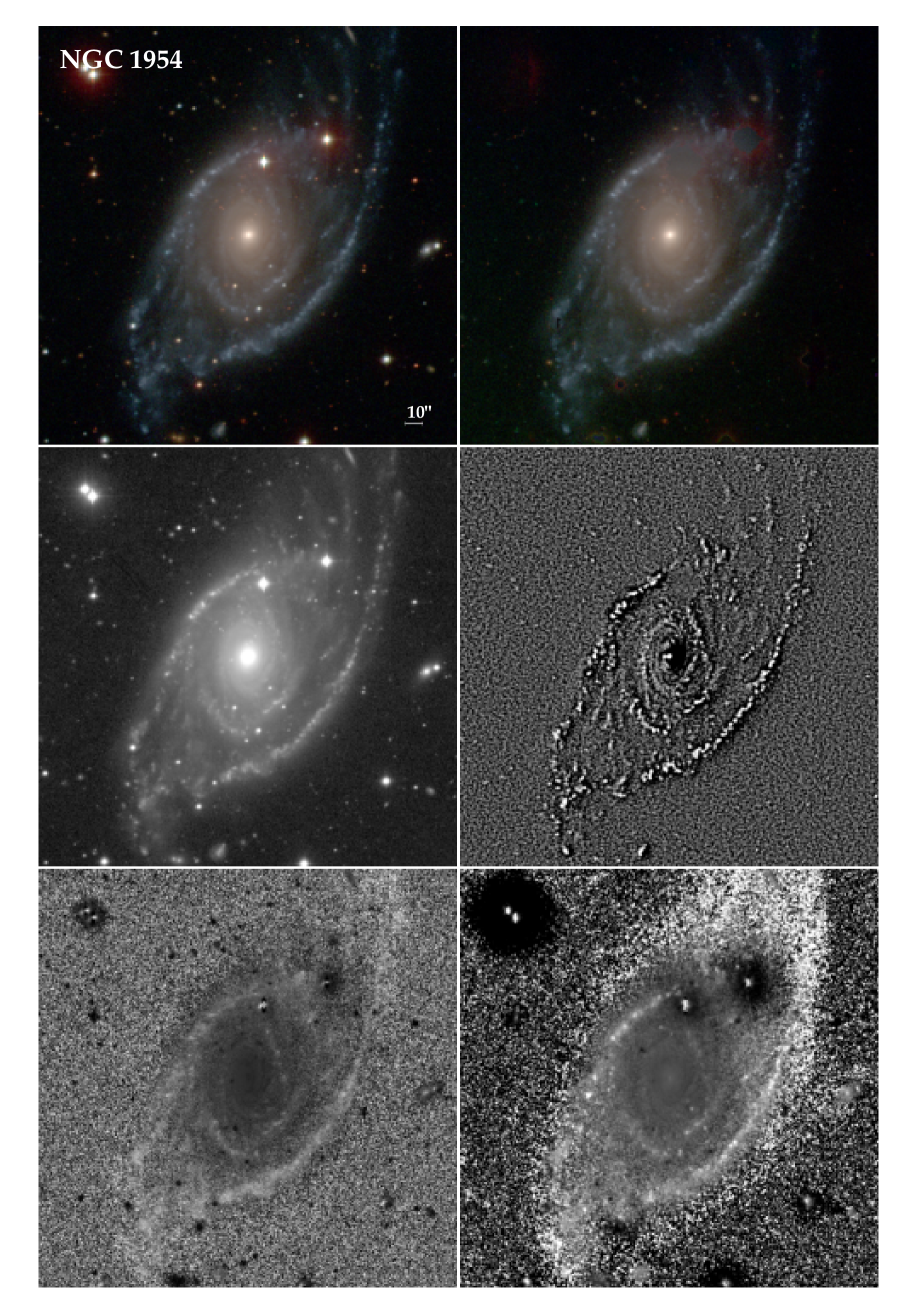
Figure 7(a): Sample page from the image atlas, illustrating NGC 1954. The panels show, from top to bottom, left to right: the composite color image, the star-cleaned composite color image, the BVRI stacked image, the structure map of the star-cleaned $B$-band image, and the $B-R$ and $R-I$ color index maps. Darker regions on the index maps correspond to redder colors. Each image is scaled to a dimension of $1.5\,D_{25}$, with north up and east to the left. The color composite, star-cleaned, and stacked images are shown on an arcsinh stretch, and the rest are shown on a linear stretch.

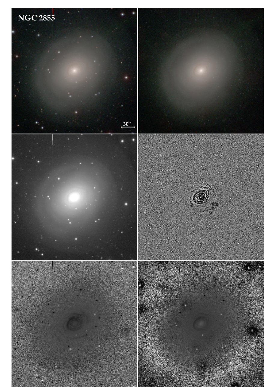
Figure 7(b): Sample page from the image atlas, illustrating NGC 2855. The panels show, from top to bottom, left to right: the composite color image, the star-cleaned composite color image, the BVRI stacked image, the structure map of the star-cleaned $B$-band image, and the $B-R$ and $R-I$ color index maps. Darker regions on the index maps correspond to redder colors. Each image is scaled to a dimension of $1.5\,D_{25}$, with north up and east to the left. The color composite, star-cleaned, and stacked images are shown on an arcsinh stretch, and the rest are shown on a linear stretch.

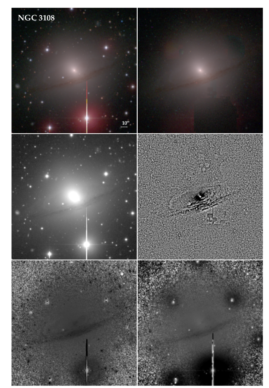
Figure 7(c): Sample page from the image atlas, illustrating NGC 3108. The panels show, from top to bottom, left to right: the composite color image, the star-cleaned composite color image, the BVRI stacked image, the structure map of the star-cleaned $B$-band image, and the $B-R$ and $R-I$ color index maps. Darker regions on the index maps correspond to redder colors. Each image is scaled to a dimension of $1.5\,D_{25}$, with north up and east to the left. The color composite, star-cleaned, and stacked images are shown on an arcsinh stretch, and the rest are shown on a linear stretch.

References

- Aguerri et al. (2005) Aguerri, J. A. L., Elias-Rosa, N., Corsini, E. M., & Muñoz-Tuñón, C. 2005, A&A, 434, 109
- Andredakis & Sanders (1994) Andredakis, Y. C., & Sanders, R. H. 1994, MNRAS, 267, 283
- Athanassoula (2003) Athanassoula, E. 2003, MNRAS, 341, 1179
- Athanassoula (2005) Athanassoula, E. 2005, MNRAS, 358, 1477
- Barazza et al. (2008) Barazza, F. D., Jogee, S., & Marinova, I. 2008, ApJ, 675, 1194
- Barth (2007) Barth, A. J. 2007, AJ, 133, 1085
- Beard & MacGillivray (1990) Beard, S. M., & MacGillivray, H. T. 1990, MNRAS, 247, 311
- Bertin & Arnouts (1996) Bertin, E., & Arnouts, S. 1996, A&AS, 117, 393
- Blanton et al. (2003) Blanton, M. R., Hogg, D. W., Bahcall, N. A., et al. 2003, ApJ, 592, 819
- Böker et al. (2003) Böker, T., Stanek, R., & van der Marel, R. P. 2003, AJ, 125, 1073
- Böker et al. (2002) Böker, T., van der Marel, R. P., Laine, S., et al. 2002, AJ, 123, 1389
- Bottinelli et al. (1995) Bottinelli, L., Gouguenheim, L., Paturel, G., & Teerikorpi, P. 1995, A&A, 296, 64
- Bournaud et al. (2005) Bournaud, F., Combes, F., Jog, C. J., & Puerari, I. 2005, A&A, 438, 507
- Buat et al. (2007) Buat, V., Takeuchi, T. T., Iglesias-Páramo, J., et al. 2007, ApJS, 173, 404
- Bureau & Freeman (1999) Bureau, M., & Freeman, K. C. 1999, AJ, 118, 126
- Buta & Crocker (1991) Buta, R., & Crocker, D. A. 1991, AJ, 102, 1715
- Buta et al. (2006) Buta, R., Laurikainen, E., Salo, H., Block, D. L., & Knapen, J. H. 2006, AJ, 132, 1859
- Carollo et al. (1997) Carollo, C. M., Stiavelli, M., de Zeeuw, P. T., & Mack, J. 1997, AJ, 114, 2366
- Courteau (1996) Courteau, S. 1996, ApJS, 103, 363
- Courteau et al. (1996) Courteau, S., de Jong, R., & Broeils, A. 1996, ApJ, 457, L73
- Crook et al. (2007) Crook, A. C., Huchra, J. P., Martimbeau, N., Masters, K. L., Jarrett, T., & Macri, L. M. 2007, ApJ, 655, 790
- Dale et al. (2007) Dale, D. A., Gil de Paz, A., Gordon, K. D., et al. 2007, ApJ, 655, 863
- de Jong (1996) de Jong, R. S. 1996, A&AS, 118, 557
- de Vaucouleurs (1948) de Vaucouleurs, G. 1948, Ann. d’Ap., 11, 247
- de Vaucouleurs et al. (1991) de Vaucouleurs, G., de Vaucouleurs, A., Corwin Jr., H. G., et al. 1991, Third Reference Catalogue of Bright Galaxies (New York: Springer) (RC3)
- Erwin et al. (2005) Erwin, P., Beckman, J. E., & Pohlen, M. 2005, ApJ, 626, L81
- Erwin et al. (2008) Erwin, P., Pohlen, M., & Beckman, J. E. 2008, AJ, 135, 20
- Eskridge et al. (2002) Eskridge, P. B., Frogel, J. A., Pogge, R. W., et al. 2002, ApJS, 143, 73
- Ferguson (1989) Ferguson, H. C. 1989, AJ, 98, 367
- Ferguson & Sandage (1990) Ferguson, H. C., & Sandage, A. 1990, AJ, 100, 1
- Forbes et al. (1995) Forbes, D. A., Franx, M., & Illingworth, G. D. 1995, AJ, 109, 1988
- Freeman (1970) Freeman, K. C. 1970, ApJ, 160, 811
- Frei (1996) Frei, Z. 1996, PASP, 108, 624
- Frei et al. (1996) Frei, Z., Guhathakurta, P., Gunn, J. E., & Tyson, J. A. 1996, AJ, 111, 174
- Frei & Gunn (1994) Frei, Z., & Gunn, J. E. 1994, AJ, 108, 1476
- Friedli & Benz (1993) Friedli, D., & Benz, W. 1993, A&A, 268, 65
- Fukugita et al. (1995) Fukugita, M., Shimasaku, K., & Ichikawa, T. 1995, PASP, 107, 945
- Gadotti (2009) Gadotti, D. A. 2009, MNRAS, 393, 1531
- Gavazzi et al. (2003) Gavazzi, G., Boselli, A., Donati, A., Franzetti, P., & Scodeggio, M. 2003, A&A, 400, 451
- Gawiser et al. (2006) Gawiser, E., van Dokkum, P. G., Herrera, D., et al. 2006, ApJS, 162, 1
- Gil de Paz et al. (2007) Gil de Paz, A., Boissier, S., Madore, B. F., et al. 2007, ApJS, 173, 185
- Gott (1977) Gott, J. R., III 1977, ARA&A, 15, 235
- Graham & Worley (2008) Graham, A. W., & Worley, C. C. 2008, MNRAS, 388, 1708
- Helou et al. (1988) Helou, G., Khan, I. R., Malek, L., & Boehmer, L. 1988, ApJS, 68, 151
- Ho et al. (1995) Ho, L. C., Filippenko, A. V., & Sargent, W. L. W. 1995, ApJS, 98, 477
- Ho et al. (1997a) Ho, L. C., Filippenko, A. V., & Sargent, W. L. W. 1997a, ApJS, 112, 315
- Ho et al. (1997b) Ho, L. C., Filippenko, A. V., & Sargent, W. L. W. 1997b, ApJ, 487, 59
- Hubble (1926) Hubble, E. 1926, ApJ, 64, 321
- Jansen et al. (2000) Jansen, R. A., Franx, M., Fabricant, D., & Caldwell, N. 2000, ApJS, 126, 271
- Jarrett et al. (2003) Jarrett, T. H., Chester, T., Cutri, R., Schneider, S., & Huchra, J. P. 2003, AJ, 125, 525
- Kent (1985) Kent, S. M. 1985, ApJS, 59, 115
- Kormendy (1985) Kormendy, J. 1985, ApJ, 292, L9
- Kormendy & Barentine (2010) Kormendy, J., & Barentine, J. C. 2010, ApJ, 715, L176
- Kormendy et al. (2009) Kormendy, J., Fisher, D. B., Cornell, M. E., & Bender, R. 2009 ApJS, 182, 216
- Kormendy & Kennicutt (2004) Kormendy, J., & Kennicutt, R. C. 2004, ARA&A, 42, 603
- Landolt (1992) Landolt, A. U. 1992, AJ, 104, 372
- Lang et al. (2010) Lang, D., Hogg, D. W., Mierle, K., Blanton, M., & Roweis, S. 2010, AJ, 139, 1782
- Lasker et al. (2008) Lasker, B. M., Lattanzi, M. G., McLean, B. J., et al. 2008, AJ, 136, 735
- Lauer (1985) Lauer, T. R. 1985, ApJ, 292, 104
- Lauer et al. (1995) Lauer, T. R., Ajhar, E. A., Byun, Y.-I., et al. 1995, AJ, 110, 2622
- Laurikainen et al. (2005) Laurikainen, E., Salo, H., & Buta, R. 2005, MNRAS, 362, 1319
- Ledo et al. (2010) Ledo, H. R., Sarzi, M., Dotti, M., Khochfar, S., & Morelli, L. 2010, MNRAS, 407, 969
- Levine & Sparke (1998) Levine, S. E., & Sparke, L. S. 1998, ApJ, 496, L13
- Li et al. (2011) Li, Z.-Y., Ho, L. C., Barth, A. J., & Peng, C. Y. 2011, ApJS, in press (Paper II)
- Lin & Pringle (1987) Lin, D. C., & Pringle, J. E. 1987, ApJ, 320, L87
- Lupton et al. (2004) Lupton, R. H., Blanton, M. R., Fekete, G., et al. 2004, PASP, 116, 133
- Lütticke et al. (2000) Lütticke, R., Dettmar, R.-J., & Pohlen, M. 2000, A&AS, 145, 405
- MacArthur et al. (2003) MacArthur, L., Courteau, S., & Holtzman, J. A. 2003, ApJ, 582, 689
- Montgomery et al. (1993) Montgomery, K. A., Marschall, L. A., and Janes, K. A., 1993, AJ, 106, 181
- Murali et al. (2002) Murali, C., Katz, N., Hernquist, L., Weinberg, D. H., & Davé, R. 2002, ApJ, 571, 1
- Noordermeer & van der Hulst (2007) Noordermeer, E., & van der Hulst, J. M. 2007, MNRAS, 376, 1480
- Paturel et al. (1997) Paturel, G., Andernach, H., Bottinelli, L., et al. 1997, A&AS, 124, 109
- Paturel et al. (2003) Paturel, G., Petit, C., Prugniel, Ph., et al. 2003, A&A, 412, 45
- Peletier & de Grijs (1998) Peletier, R. F., & de Grijs, R. 1998, MNRAS, 300, L3
- Peng et al. (2002) Peng, C. Y., Ho, L. C., Impey, C. D., & Rix, H.-W. 2002, AJ, 124, 266
- Peng et al. (2010) Peng, C. Y., Ho, L. C., Impey, C. D., & Rix, H.-W. 2010, AJ, 139, 2097
- Pogge & Martini (2002) Pogge, R. W., & Martini, P. 2002, ApJ, 569, 624
- Ravindranath et al. (2001) Ravindranath, S., Ho, L. C., Peng, C. Y., Filippenko, A. V., & Sargent, W. L. W. 2001, AJ, 122, 653
- Rice et al. (1988) Rice, W., Lonsdale, C. J., Soifer, B. T., et al. 1988, ApJS, 68, 91
- Rix & White (1992) Rix, H.-W., & White, S. D. M. 1992, MNRAS, 254, 389
- Roberts (1962) Roberts, M. S. 1962, AJ, 67, 437
- Sanders et al. (2003) Sanders, D. B., Mazzarella, J. M., Kim, D.-C., Surace, J. A., & Soifer, B. T. 2003, AJ, 126, 1607
- Schlegel et al. (1998) Schlegel, D. J., Finkbeiner, D. P., & Davis, M. 1998, ApJ, 500, 525
- Schmidt (1968) Schmidt, M. 1968, ApJ, 151, 393
- Schombert (1986) Schombert, J. M. 1986, ApJS, 60, 603
- Seigar et al. (2002) Seigar, M., Carollo, C. M., Stiavelli, M., de Zeeuw, T., & Dejonghe, H. 2002, AJ, 123, 184
- Sérsic (1968) Sérsic, J. L. 1968, Atlas de Galaxias Australes (Córdoba: Obs. Astron., Univ. Nac. Córdoba)
- Sheth et al. (2010) Sheth, K., Regan, M., Hinz, J. L., et al. 2010, PASP, 122, 1397
- Skrutskie et al. (2006) Skrutskie, M. F., Cutri, R. M., Stiening, R., et al. 2006, AJ, 131, 1163
- Thilker et al. (2005) Thilker, D. A., Bianchi, L., Boissier, S., et al. 2005, ApJ, 619, L79
- Tran et al. (2001) Tran, H. D., Tsvetanov, Z., Ford, H. C., et al. 2001, AJ, 121, 2928
- van Albada (1982) van Albada, T. S. 1982, MNRAS, 201, 939
- van der Kruit (1979) van der Kruit, P. C. 1979, A&AS, 38, 15
- van Dokkum (2001) van Dokkum, P. G. 2001, PASP, 113, 1420
- van Dokkum (2005) van Dokkum, P. G. 2005, AJ, 130, 2647
- van Dokkum & Franx (1995) van Dokkum, P. G., & Franx, M. 1995, AJ, 110, 2027
- Wyse et al. (1997) Wyse, R. F. G., Gilmore, G., & Franx, M. 1997, ARA&A, 35, 637
- York et al. (2000) York, D. G., Adelman, J., Anderson Jr., J. E., et al. 2000, AJ, 120, 1579
- Zaritsky & Rix (1997) Zaritsky, D., & Rix, H.-W. 1997, ApJ, 477, 118