Stable regimes for hard disks in a channel with twisting walls

Abstract.

We study a gas of $N$ hard disks in a box with semi-periodic boundary conditions. The unperturbed gas is hyperbolic and ergodic (these facts are proved for $N=2$ and expected to be true for all $N\geq 2$). We study various perturbations by twisting the outgoing velocity at collisions with the walls. We show that the dynamics tends to collapse to various stable regimes, however we define the perturbations and however small they are.

Keywords: Hard balls, hard disks, hyperbolicity, ergodicity, stability, nonequilibrium dynamics, steady states, SRB measures.

Gas of hard balls is a classical model of statistical mechanics. The chaotic motion of its molecules can explain many phenomena observed in real gases and fluids. We study a 2D gas of hard disks placed in a channel whose walls act as “Maxwell demon” that makes the angle of reflection different from the angle of incidence (twisting the outgoing velocity vectors). We present quite unexpected patterns developed by the gas dynamics under various twisting rules.

1. Introduction

The gas of hard balls is a classical model of statistical mechanics. Hard ball collisions produce strong scattering effect which makes the system behave chaotically and quickly relax to equilibrium (at least locally). In mathematical terms, the gas of hard balls in finite container is widely regarded as a hyperbolic dynamical system (i.e., its Lyapunov exponents should not be zero) and its natural invariant measure (Liouville measure) is expected to be ergodic and mixing.

More precisely, the celebrated Boltzmann-Sinai ergodic hypothesis states that the gas of $N$ hard balls in a container with periodic boundary conditions (a torus) is hyperbolic, ergodic, mixing (and Bernoulli). Attempts to prove this conjecture have long history [28, 29, 30], and at present it is proven under various conditions [15, 24, 25, 26, 27], but not yet in its full generality.

We note that the gas of $N$ hard balls on a $d$-dimensional torus has $d+1$ integrals of motion: its kinetic energy and its total momentum (a $d$-vector) are preserved, hence the position of the center of mass can be fixed. This leads to a great reduction of the phase space eliminating a total of $2d+1$ dimensions.

If the container has rigid walls, the total momentum is no longer preserved, thus the phase space has higher dimensionality and is more complicated; such gases are even harder to study. Hyperbolicity and ergodicity have been proven only for $N=2$ balls in a rectangular box (when the disks are no too large) [23] and for $N\geq 2$ disks in a very special 2D container with curved walls where each disk is confined to its own cell [5].

We are interested in a gas of $N$ hard disks in a 2D rectangular container with partial periodicity, i.e., where two opposite walls are rigid but in the other direction boundary conditions are periodic (such a container can be regarded as a cylinder, rather than a torus). The hyperbolicity and ergodicity for such a gas are proved only for $N=2$, see [23], but these properties are undoubtedly valid for all $N\geq 2$.

The dynamics of this gas becomes more intriguing if small driving forces are added at the rigid walls, i.e., when collisions of the disks with the walls are modified by stochastic or deterministic perturbations. We consider deterministic perturbations where the angle of reflection is no longer equal to the angle of incidence, i.e., the velocity vector of the colliding disk is “twisted” a little right after the collision. Such twisting collision rules may appear physically unrealistic (they belong to the “Maxwell-demon” type of external forces), but they produce very realistic and interesting nonequilibrium phenomena such as shear flow and entropy production [7].

It is commonly expected (and observed empirically [7]) that the gas of hard balls under small perturbations remains chaotic and has a unique nonequilibrium stationary state, perhaps in the form of a Sinai-Ruelle-Bowen (SRB) measure, i.e., an ergodic measure with smooth conditional densities on unstable manifolds. These facts have been actually proven for $N=1$ particle in the the 2D periodic Lorentz gas under two types of small perturbations: external fields [6, 10, 12] and twisting collision rules [32]. Similar results were obtained for various classes of bounded billiard tables with twisting walls [1, 17].

We note that the unperturbed Lorentz gas with $N=1$ particle is a uniformly hyperbolic dynamical system. Under small perturbations, uniform hyperbolicity usually survives and makes the construction of an SRB measure possible.

The gas of $N\geq 2$ hard balls, on the other hand, is never uniformly hyperbolic. Non-uniform hyperbolicity can be easily destroyed even by arbitrary small perturbations making it hard to control the perturbed dynamics. For this reason there are no theoretical proofs of hyperbolicity or the existence of SRB measures under any perturbations, to our knowledge. Moreover, one may expect that the perturbed gas is not always fully hyperbolic or ergodic, i.e., that there may be elliptic islands or multiple ergodic components, etc.

The modest purpose of this paper is to point out that things are actually much worse, even for the gas of $N=2$ disks. We show that if the disks are not too big (if their diameters are less than 0.5), then an arbitrarily small twist added to collisions at the walls tends to destroy the chaotic behavior of the gas causing a complete collapse of the dynamics in a way that almost every phase trajectory converges to some trivial stable regimes. The collapse seems to happen for every type of small twists, though the limit stable regimes may be very different and sometimes quite bizarre.

Most of the stable regimes we observed for $N=2$ also appear for any number $N>2$ of disks (provided their diameter is small enough). On the other hand, when the disks are not too small, then our stable regimes seem to disappear. We believe that if the diameters of the disks are greater than $1/N$, then the gas is fully chaotic and SRB measures exist, in agreement with numerical evidence [7].

This work is motivated by discussions with J. Lebowitz and Ya. Sinai. Our original purpose was to prove hyperbolicity and construct SRB measures for at least some types of twisting collisions. However, we discovered that at sufficiently low densities all twists cause a total collapse (often to our surprise). Thus in the end we decided to report our findings in this paper.

2. Model

Our model is a system of $N$ hard disks in a unit square

$$D=\{0\leq x\leq 1,\ \ 0\leq y\leq 1\}$$

that has rigid (reflecting) walls at $y=0$ and $y=1$ and periodic boundary conditions at $x=0$ and $x=1$. The disks are identical (have the same mass and radius), and they collide elastically with each other.

We can represent our model as an infinite chain of copies of the square $D$ placed in the infinite strip (channel) $I=\{0\leq y\leq 1\}$ where hard disks appear periodically; see Fig. 1.

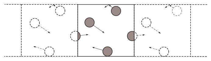
Figure 1. A periodic system of disks moving in a channel.

We denote by $\mathbf{q}_{i}=(x_{i},y_{i})$ the position of the $i$th disk and by $\mathbf{p}_{i}=(u_{i},v_{i})$ its velocity vector, $i=1,\ldots,N$. Now suppose a disk collides with a wall (either $y=0$ or $y=1$). By the classical law its velocity $\mathbf{p}=\mathbf{p}_{\rm before}=(u,v)$ changes to $\mathbf{p}_{\rm after}=(u,-v)$, and its kinetic energy $\tfrac{1}{2}\|\mathbf{p}\|^{2}$ is preserved, i.e.,

(2.1) $$\|\mathbf{p}_{\rm before}\|=\|\mathbf{p}_{\rm after}\|.$$

The total momentum $\mathbf{p}_{\rm total}=\mathbf{p}_{1}+\cdots+\mathbf{p}_{N}$ of the system is not preserved, but its $x$-component is preserved, i.e., the sum $u_{1}+\cdots+u_{N}$ remains constant in time.

The entire (macrocanonical) phase space is $4N$-dimensional, and the energy surface is $(4N-1)$-dimensional. The conservation of $u_{1}+\cdots+u_{N}$ allows us to set it to zero, after which the $x$-coordinate of the center of mass will be constant and can be fixed, too. Thus the reduced phase space is $(4N-3)$-dimensional. The resulting system is expected to be hyperbolic (with $2N-2$ positive Lyapunov exponents and the same number of negative ones), ergodic, and mixing. These facts have been proved for $N=2$ in [23].

We now modify the law of collisions with the walls. We will preserve the kinetic energy of the disks, so that (2.1) still holds true. Thus it is enough to specify the angle of reflection $\psi$, as a function of the angle of incidence, $\varphi$:

(2.2) $$\psi=f(\varphi).$$

We measure the angles $\psi$ and $\varphi$ as shown in Figure 2, so that the range of our angles is the interval $[0,\pi]$. The function $f$ does not depend on the point of collision, but it may be different for the bottom wall at $y=0$ and the top wall at $y=1$. We will denote those two functions by $f_{0}$ and $f_{1}$, respectively.

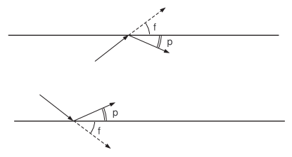
Figure 2. Angle of incidence $\varphi$ and angle of reflection $\psi$.

For classical collisions $\psi=\varphi$, hence $f$ is the identity function, $f(\varphi)=\varphi$. We will consider its small perturbations, i.e., our functions $f$ will satisfy $f(\varphi)=\varphi+\,{\rm small}$. For convenience we also assume that

• $f(\varphi)$ is continuous and strictly monotonically increasing;

• $f(0)=0$ and $f(\pi)=\pi$,

i.e., $f$ is an orientation preserving homeomorphism of the interval $[0,\pi]$. This ensures that our dynamics will be invertible, i.e., every phase point has a unique past.

As before, the energy surface in the phase space is $(4N-1)$-dimensional. Since our collision rules are translation invariant (independent of the $x$ coordinate of the collision point), the energy surface is naturally foliated by invariant hypersurfaces on which the dynamics are identical. Thus we can factor this foliation out by replacing the $x$-coordinates of the disks by their relative $x$-coordinates $x_{1}-x_{n}$, $\ldots$, $x_{n-1}-x_{n}$, which eliminates one more variable and makes the (factored) phase space $(4N-2)$-dimensional. Most of the time we will deal with $N=2$ disks, in which case the phase space will be 6-dimensional.

Many collision rules (2.2) quickly lead to trivial degenerate regimes. For example, if $f_{k}(\varphi)<\varphi$ for $k=0,1$ and all $0<\varphi<\pi$, then $u_{\rm after}=\cos\psi>\cos\varphi=u_{\rm before}$, hence the $x$-component of the total momentum, $u_{\rm total}=u_{1}+\cdots+u_{N}$ will grow at every collision with the walls. It is then clear that all the particles will eventually move almost horizontally to the right (will be “blown away by wind”).

To prevent the wind from blowing, we will restrict our study to collision rules where one wall counterbalances the effect of the other:

(2.3) $$f_{1}(\varphi)=\pi-f_{0}(\pi-\varphi),$$

i.e., the function $f_{1}$ at the top wall $y=1$ acts exactly opposite to the function $f_{0}$ at the bottom wall $y=0$. Under this condition there is a natural symmetry in the channel, hence drift in either direction (left or right) cannot be dominant in the whole phase space.

3. One particle case

To clarify the effect of our twisting collisions, we begin with the simplest case of one hard disk, i.e., we set $N=1$. Then the radius of the disk is irrelevant, and we can just make it a point particle bouncing between the two walls.

Let $\varphi_{0}$ be the angle of incidence at the initial collision at, say, the bottom wall $y=0$. Then the reflection angle $\psi=f_{0}(\varphi_{0})$ becomes the incidence angle $\varphi_{1}$ at the next collision at the top wall, i.e., $\varphi_{1}=f_{0}(\varphi_{0})$. Similarly, the incidence angle at the following collision at the bottom wall will be

$$\varphi_{2}=f_{1}(\varphi_{1})=f_{1}(f_{0}(\varphi_{0})),$$

and then the process will repeat periodically. By induction,

$$\varphi_{2n}=g^{n}(\varphi_{0})\qquad\text{for all}\quad n\geq 1,$$

where $g=f_{1}\circ f_{0}$, thus the evolution of incidence angles is completely described by the iterations of the function $g$. For functions with opposite orientations, i.e., those obeying (2.3), we have

(3.1) $$g(\varphi)=\pi-f_{0}\bigl{(}\pi-f_{0}(\varphi)\bigr{)}.$$

Note that $g$, just like $f_{0}$, is an orientation-preserving homeomorphism of the interval $[0,\pi]$. But not any homeomorphism of $[0,\pi]$ can be defined by (3.1), so we describe the class of functions $g$ satisfying (3.1). To this end we introduce an involution $j\colon[0,\pi]\to[0,\pi]$ defined by $j(\varphi)=\pi-\varphi$ and note that

$$g=(j\circ f_{0})\circ(j\circ f_{0})$$

Thus, $g=h^{2}$, where $h=j\circ f_{0}$ is an orientation reversing homeomorphism of the interval $[0,\pi]$.

The map $h\colon[0,\pi]\to[0,\pi]$ obviously has a unique fixed point $\varphi_{0}\in(0,\pi)$, which automatically is a fixed point for $g$. For any other point $\varphi\neq\varphi_{0}$ there are exactly three possibilities:

• $h^{2}(\varphi)=\varphi$, then $\varphi$ is a 2-periodic point for $h$ and a fixed point for $g$;

• $|h^{2}(\varphi)-\varphi_{0}|<|\varphi-\varphi_{0}|$, then the images of $\varphi$ under $g$ will move toward $\varphi_{0}$;

• $|h^{2}(\varphi)-\varphi_{0}|>|\varphi-\varphi_{0}|$, then the images of $\varphi$ under $g$ will move away from $\varphi_{0}$;

The non-fixed points of $g$ make an open set, which is a union of disjoint intervals, we denote them by $\{I_{m}\}$. The endpoints of each interval $I_{m}$ are fixed points for $g$, i.e., 2-periodic points for $h$ (unless one of them is $\varphi_{0}$, of course). In each interval $I_{m}\subset[0,\pi]$ all the points move under $g$ in one direction – either toward $\varphi_{0}$ or away from $\varphi_{0}$.

For each interval $I_{m}$ its image $I_{m^{\prime}}=h(I_{m})$ is another interval whose points move in the same direction (either toward $\varphi_{0}$ or away from $\varphi_{0}$) as the points of $I_{m}$. Note that $I_{m}=h(I_{m^{\prime}})$ as well. We call the intervals $I_{m}$ and $I_{m^{\prime}}$ dual to each other. Thus the intervals $\{I_{m}\}$ come in dual pairs. Dual intervals lie on the opposite sides of $\varphi_{0}$, and all the points in both intervals move either toward $\varphi_{0}$ or away from $\varphi_{0}$. If $I_{m},I_{m^{\prime}}$ and $I_{n},I_{n^{\prime}}$ are two pairs of dual intervals, then one pair lies inside the other; see Figure 3.

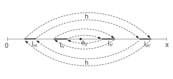
Figure 3. Dual intervals about the fixed point $\varphi_{0}$.

If the number of intervals $I_{m}$ is finite, then it is necessarily even, and exactly half of them lies to the left of $\varphi_{0}$, and the other half – to the right. The above structure is essentially a complete description of all interval maps $g$ satisfying (3.1):

Proposition 3.1.

Let $g$ be an orientation preserving homeomorphism of the interval $[0,\pi]$ with an odd number of fixed points

$$0=\varphi_{-k}<\varphi_{-k+1}<\cdots<\varphi_{0}<\cdots\varphi_{k-1}<\varphi_{k}=\pi.$$

Suppose that for each $0\leq i<k$ either all the points of both intervals $(\varphi_{-i-1},\varphi_{-i})$ and $(\varphi_{i},\varphi_{i+1})$ move under $g$ toward $\varphi_{0}$ or all the points in these two intervals move away from $\varphi_{0}$. Then there exists an orientation reversing homeomorphism $h\colon[0,\pi]\to[0,\pi]$ such that $g=h^{2}$. The middle fixed point $\varphi_{0}$ is the (only) fixed point of $h$.

The proof uses standard methods of one-dimensional topological dynamics, and we omit it.

The central fixed point $\varphi_{0}$ plays a special role, we will call it the center (of the map $g$); it is the only fixed point of $h$. Note that

(3.2) $$f_{0}(\varphi_{0})=\pi-\varphi_{0},$$

hence if a particle hits a wall at the angle $\varphi_{0}$, it turns around and flies straight back. Its trajectory is then periodic not only in the angular coordinates, but also in the spatial coordinates; see Fig. 4.

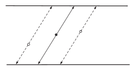
Figure 4. A periodic trajectory running between two collisions.

4. A special family of collisions with a twist

While most of our conclusions apply to generic functions $f_{0}$ and $f_{1}$ satisfying (2.3), it will be convenient to use one particular family of functions to clarify our arguments.

First, it is convenient when the center $\varphi_{0}$ is at the geometric center of the interval $[0,\pi]$, i.e., $\varphi_{0}=\pi/2$. Then the special periodic trajectories described in the end of Section 3 move vertically, up and down, i.e., they just bounce between the walls like the regular periodic billiard trajectories.

Next, for simplicity we consider functions $g$ that have one fixed point $\varphi_{0}=\pi/2$ (other than $0$ and $\pi$), which will automatically be the center. Then there are three fixed points total: $0,\pi/2$, and $\pi$. The intervals $(0,\pi/2)$ and $(\pi/2,\pi)$ either both move toward $\pi/2$ or both move away from $\pi/2$. In the former case $\pi/2$ will be a stable fixed point and attract the entire interval $(0,\pi)$. In the latter case $\pi/2$ will be an unstable (repulsive) fixed point and then each interval $(0,\pi/2)$ and $(\pi/2,\pi)$ will be attracted by its other endpoint, i.e., by $0$ or $\pi$, respectively. We will say that in the former case the map $g$ has a stable center and in the latter – an unstable center. These cases are quite different, in dynamical terms, and both are interesting.

We note that in order to make $\pi/2$ a fixed point for $g$ satisfying (3.1), we need to set $f_{0}(\pi/2)=\pi/2$, according to (3.2). Then $\pi/2$ is a fixed point for $f_{0}$ as well.

Thus $f_{0}$ must have three fixed points: $0$, $\pi/2$, and $\pi$. It is also convenient if the time reversal of the collision rule defined by $f_{0}$ belongs to the same family of collision rules. The time reversal collision rule is defined by $\varphi\mapsto f_{0}^{-}(\varphi)$ at the bottom wall and $\varphi\mapsto f^{-}_{1}(\varphi)$ at the top wall, where the functions $f_{0}^{-}$ and $f_{1}^{-}$ satisfy

(4.1) $$f_{0}^{-}=f^{-1}_{1}\qquad\text{and}\qquad f_{1}^{-}=f^{-1}_{0}$$

in accordance with (2.3).

In view of the above requirement we can define $f_{0}$ by

(4.2) $$\tan f_{0}(\varphi)=e^{\lambda}\tan\varphi.$$

Then, due to (2.3),

(4.3) $$f_{1}(\varphi)=f_{0}(\varphi)$$

so both walls obey the same collision rule! Note that there are no restriction on $\lambda$ here, our rules work well for any $\lambda\in(-\infty,\infty)$, but for the twist to be small we will only consider $\lambda\approx 0$.

Due to (4.1), the time reversal collision rules satisfy

$$\tan f_{0}^{-}(\varphi)=\tan f_{1}^{-}(\varphi)=e^{-\lambda}\tan\varphi,$$

hence it belongs to the same family of rules (4.2), but $\lambda$ must be replaced with $-\lambda$, i.e., reversing the time corresponds to negating $\lambda$.

A direct differentiation of (4.2) gives

$$f_{0}^{\prime}(\varphi)=e^{-\lambda}\,\frac{\sin^{2}f_{0}(\varphi)}{\sin^{2}\varphi}=e^{\lambda}\,\frac{\cos^{2}f_{0}(\varphi)}{\cos^{2}\varphi},$$

Hence

$$f_{0}^{\prime}(\pi/2)=e^{-\lambda}\qquad\text{and}\qquad f_{0}^{\prime}(0)=f_{0}^{\prime}(\pi)=e^{\lambda}.$$

Thus, $\lambda>0$ corresponds to a stable center and $\lambda<0$ to an unstable center, i.e., we have dynamics of both types.

We note that the rules (4.2)–(4.3) can be rewritten as follows: at every collision with the wall the incoming velocity $(u^{-},v^{-})$ and the outgoing velocity $(u^{+},v^{+})$ are related by

(4.4) $$u^{+}/|v^{+}|=e^{-\lambda}u^{-}/|v^{-}|.$$

This makes it convenient for numerical simulations: one can recompute the velocity vectors by (4.4) without using the angle $\varphi$ or its tangent.

5. Collisions with a stable center

We begin with a single disk and a small positive $\lambda>0$. Again, we assume that the disk has zero radius, i.e., it is just a point particle.

Recall that $f_{0}^{\prime}(\pi/2)=e^{-\lambda}<1$. Thus if the angle of incidence is close to $\pi/2$, i.e., $\varphi=\pi/2+\delta$ for some small $\delta$, then after $n$ collisions at the walls it will be $\varphi_{n}=\pi/2+\delta_{n}$, where $\delta_{n}\to 0$.

More precisely, as the disk moves between collisions from wall to wall, its displacement in the horizontal direction is given by $\Delta x=\cot\varphi=\tan\delta$. Due to (4.2)–(4.3), after the next collision its displacement will be $e^{-\lambda}\cot\varphi=e^{-\lambda}\,\Delta x$. Thus the displacement in the $x$ direction is precisely decreasing by a factor $e^{-\lambda}<1$.

Thus the displacements in the $x$ direction make a geometric progression and the total displacement is

(5.1) $$\Delta x\sum_{n=0}^{\infty}e^{-n\lambda}=\frac{\Delta x}{1-e^{-\lambda}}$$

The particle’s trajectory converges to a vertical line and the velocity vector aligns vertically at an exponential rate.

Consider now the system of $N$ disks. We assume that the diameter $d$ of the disks is small enough so that the disks can be lined up along one vertical or horizontal line in the unit square, i.e., $d<1/N$.

For any disk with center at $(x_{i},y_{i})$ and velocity vector $(u_{i},v_{i})$ denote by $s_{i}$ the total displacement in the $x$ direction of that disk if it is allowed to bounce between the walls alone, as if the other disks did not exist. By (5.1), $s_{i}$ is finite, and in fact

(5.2) $$s_{i}\sim\frac{|u|}{|v|(1-e^{-\lambda})}$$

Let $U$ be the the subset in phase space satisfying the following condition:

(5.3) $$|x_{i}-x_{j}|>d+s_{i}+s_{j}\qquad\forall i\neq j$$

(note that the $x$ coordinates must be taken modulo 1, as we have periodic boundary conditions at $x=0$ and $x=1$).

Now (5.3) guarantees that the projections of the disks onto the $x$-axis do not overlap and will not overlap at any time in the future. Thus our $N$ disks will never collide with each other, all of them will be bouncing between the walls and the trajectory of each disk will converge to some vertical line.

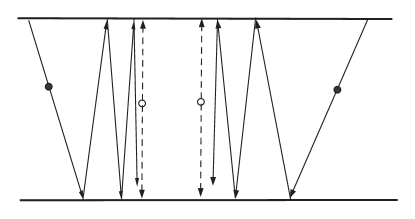
Figure 5. Convergence the a stable limit regime.

In this limit regime, the $x$-component of the velocity vector of each disk is zero. Thus those limit trajectories form a family of codimension $N$ in phase space. Note that the phase space of our system is $(4N-1)$-dimensional (the only constraint is the conservation of the total kinetic energy). Thus our family of stable limit trajectories is a $(3N-1)$-dimensional submanifold in the phase space. We denote it by $S$.

Every phase trajectory starting in $U$ converges to $S$ at an exponential rate. The set $U$ is invariant, i.e., all the trajectories originating in $U$ stay there in the future. Note that $U$ is an open subset of the phase space, thus it has a positive Lebesgue measure. Therefore the limit set $S$ has an open basin of attraction of positive Lebesgue measure.

It is more convenient to work with the collision space $\mathcal{M}$ which consists of all phase states such that either some two disks collide or a disk collides with a wall. (At the moment of collision, the velocity vectors change discontinuously, and it is customary to include in $\mathcal{M}$ only the postcollisional velocity vectors). The induced map $T=T_{\lambda}\colon\mathcal{M}\to\mathcal{M}$ is called the collision map.

We denote by $\nu_{0}$ the normalized measure on $\mathcal{M}$ that is invariant under the map $T_{0}$ corresponding to $\lambda=0$. This map corresponds to the classical specular reflections at the walls (where $\psi=\varphi$), so $T_{0}$ is the collision map for the classical gas of hard disks at equilibrium. The measure $\nu_{0}$ is absolutely continuous with respect to the Lebesgue measure on $\mathcal{M}$, and it has a strictly positive density. At the collisions with the walls, the density is proportional to $\sin\varphi$ [8].

Let $U_{0}=U\cap\mathcal{M}$ denote the subset of the collision space where (5.3) holds. It is invariant under $T$, i.e., $T(U_{0})\subset U_{0}$. Its trajectories converge to the set $S_{0}=S\cap\mathcal{M}$, i.e., $U_{0}$ is the basin of attraction of $S_{0}$ under the map $T$. The basin of attraction $U_{0}$ may be regarded as a trap, or a “hole” – every phase trajectory that enters it will never come back.

6. Holes and escape rates

Dynamical systems with holes have been studied extensively in the past decades, both numerically and theoretically [2, 9, 14, 20, 22]. In particular, many researchers studied billiards with holes [3, 4, 13, 16, 19]. It is generally observed (and in many cases proved) that holes attract almost the entire phase space, i.e., almost every trajectory sooner or later enters the hole and never returns (in other words, it escapes). This phenomenon is also interpreted as the leakage of mass (phase volume) through holes so that the remaining phase space gets thinner.

The holes are usually characterized by the escape rate $\rho>0$, which basically says that the fraction of phase space that has not escaped through the holes (not leaked out) by the time $n>0$ (where $n$ is discrete time, i.e., the collision counter) decays exponentially at a rate $\rho$, i.e., it is of order $e^{-\rho n}$. More precisely, if $\mathcal{M}_{n}$ denotes the subset of the phase space $\mathcal{M}$ that has not escaped through the holes by the time $n$, then

$$\lim_{n\to\infty}\tfrac{1}{n}\,\ln{\rm Leb}(\mathcal{M}_{n})=-\rho.$$

For any phase state $X\in\mathcal{M}$ we denote by $\tau(X)$ the escape time, i.e., the time the trajectory of $X$ enters the hole. Then $\tau(X)$ has an approximate exponential distribution on $\mathcal{M}$ with parameter $\rho$ (with respect to the Lebesgue measure), and its average is $1/\rho$.

Many studies investigate how the escape through holes is affected by the size of the latter. When holes get smaller (shrink), the escape rate decreases and the escape time grows. In our case, the “hole” $U_{0}$ described above depends on the parameter $\lambda>0$. When $\lambda$ decreases, the hole $U_{0}$ shrinks and in the limit $\lambda\to 0$ the hole converges to the submanifold $S_{0}\subset\mathcal{M}$ of zero volume.

We have investigated the escape process in our model by numerical simulations. We used $N=2$ disks of diameter $d=0.1$ with the collision rules at the walls defined by (4.2)–(4.3) for various small $\lambda>0$. We have estimated the “escape time” numerically, for different $\lambda$’s. For each $\lambda$ we simulated the dynamics from $10^{5}$ randomly chosen initial states, stopping the simulations whenever the system escaped into the “hole” $U_{0}$, and computed the mean escape time $\mu_{\tau}$.

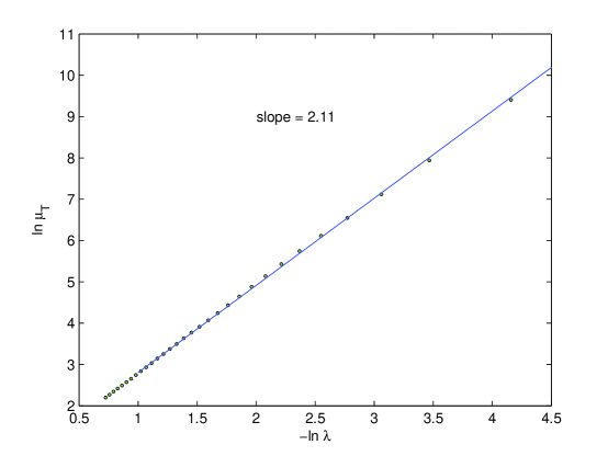
Figure 6. Plot of $\ln\mu_{\tau}$ versus $-\ln\lambda$. The least squares line has an estimated slope of 2.11.

It naturally grows, as $\lambda$ gets smaller, and Figure 6 shows how its grows on the log-log scale. The plot clearly demonstrates a linear pattern suggesting that $\mu_{\tau}\sim\lambda^{-b}$ for some $b>0$. The least squares fitting line in Figure 6 has slope 2.11, so we may guess that $b\approx 2$. Below we give a heuristic argument supporting (and refining) this conjecture.

Recall that the “hole” $U_{0}\subset\mathcal{M}$ is an open set of positive Lebesgue measure, and it is invariant under the collision map $T$, i.e., $T(U_{0})\subset U_{0}$. Hence the sets

$$U_{1}=T^{-1}(U_{0})\setminus U_{0}\qquad\text{and}\qquad U_{k}=T^{-k+1}(U_{1})$$

for $k=2,3,\ldots$ are disjoint and each of them has positive Lebesgue measure, too. Their union $U_{\infty}=\cup_{k=0}^{\infty}U_{k}$ contains all the phase points $X\in\mathcal{M}$ that end up in the hole $U_{0}$ eventually. Our first conjecture (well supported by our numerical observations) is that almost every phase point $X\in\mathcal{M}$ eventually ends up in the hole, i.e., $U_{\infty}$ covers the entire collision space $\mathcal{M}$ (up to a null set), i.e., $\mathcal{M}=U_{\infty}$ (mod 0). By direct analysis (we omit details)

(6.1) $${\rm Leb}(U_{0})=\mathcal{O}(\lambda^{N})\qquad\text{and}\qquad{\rm Leb}(U_{1})=\mathcal{O}(\lambda^{N+1}).$$

and similar estimates hold for $\nu_{0}(U_{0})$ and $\nu_{0}(U_{1})$.

Next, the measure $\nu_{0}$ is invariant under the original, twist-free collision map $T_{0}$, but not for $\lambda\neq 0$. In fact, it is preserved by the interparticle collisions, but at collisions with the walls it gets compressed if $f_{0}^{\prime}(\varphi)<1$ and gets expanded if $f_{0}^{\prime}(\varphi)>1$. In our case, $f_{0}^{\prime}(\varphi)<1$ whenever $c_{1}<\varphi<c_{2}$ for some constants $0<c_{1}<c_{2}<\pi$ whose values are not essential.

For any point $X\in\mathcal{M}$ we denote the Jacobian of the inverse collision map $T^{-1}$, with respect to the canonical measure $\nu_{0}$ by $J(X)=e^{\gamma(X)}$. If $X$ corresponds to an inter-particle collision, then $J(X)=1$, hence $\gamma(X)=0$. Otherwise $\gamma$ has a small (of order $\lambda$) value.

Now for every point $X\in U_{1}$ and $k\geq 1$ we denote

$$J_{k}(X)=J(T^{-k+1}(X))=e^{\gamma_{k}},\qquad\gamma_{k}=\gamma(T^{-k+1}(X)),$$

then we have

(6.2) $$\nu_{0}(U_{k+1})=\int_{U_{1}}J_{1}\cdots J_{k}\,d\nu_{0}=\int_{U_{1}}e^{\gamma_{1}+\cdots+\gamma_{k}}\,d\nu_{0}.$$

Next note that the sequence $\gamma_{1},\ldots,\gamma_{k}$ is determined by the collisions of the disks with the walls along the past trajectories of points $X\in U_{1}$. As time runs backwards, the disks begin colliding with each other and a chaotic regime quickly sets in. Then the distribution of every trajectory in the phase space will be fairly close to uniform (equilibrium). Thus the values of $\gamma_{n}$ could be treated as nearly independent random variables. They are all of order $\lambda$, hence the sum of $k$ of them can be expected to grow as $\lambda\sqrt{k}$, in the spirit of the the Central Limit Theorem. Thus by (6.2) we can expect that

$$\nu_{0}(U_{k+1})\sim\int_{U_{1}}e^{\lambda\sqrt{k}}\,dX\sim\lambda^{N+1}e^{\lambda\sqrt{k}},$$

as long as the chaotic regime continues. The obvious limitation $\nu_{0}(U_{k+1})\leq 1$ gives us an upper bound for $k$:

(6.3) $$k\leq\,{\rm const}\,\frac{(\ln\lambda)^{2}}{\lambda^{2}}$$

Perhaps it is more reasonable to expect that $\nu_{0}(U_{k+1})\sim 1/k$, but this would give us pretty much the same upper bound (6.3) on $k$.

Thus we see that the chaotic regime, when the particles collide and the measure of the regions $U_{k}$ tends to grow, lasts for about $\mathcal{O}\bigl{(}(\ln\lambda)^{2}/\lambda^{2}\bigr{)}$ collisions. As a result, the mean ‘escape time’ is of the same order:

(6.4) $$\mu_{\tau}=\mathcal{O}\bigl{(}(\ln\lambda)^{2}/\lambda^{2}\bigr{)}.$$

On the log-log scale $x=-\ln\lambda$ and $y=\ln\mu_{\tau}$ adopted in Figure 6 this means

(6.5) $$y=2x+2\ln x+\,{\rm const}.$$

Accordingly, we used a functional relation $y=ax+b\ln x+c$ to approximate our data plotted in Figure 6, and the least squares fit gives

$$y=1.985x+0.233\ln x+0.811.$$

The estimated slope of 1.985 is in a good agreement with the theoretically predicted slope of 2. The logarithmic coefficient 0.233 is not close to 2 in (6.5), but it is of secondary importance for the estimate (6.4).

We now investigate the dynamics beyond the bound (6.3). The measure $\mu_{0}(U_{k})$ cannot increase with $k$ forever; in fact we must have

$$\mu_{0}(U_{k})\to 0\qquad\text{as}\quad k\to\infty,$$

and moreover, $\mu_{0}(U_{k})$ should decay fast because the series $\sum_{k}\mu_{0}(U_{k})$ is summable.

Thus for large $k$ (those far exceeding the upper bound (6.3)) the dynamics cannot be chaotic: it is dominated by the collisions with the walls that compress the phase volume (when the time runs backwards). Those collisions have incidence angles close to 0 or $\pi$, so that the particles hit the walls nearly tangentially. This means that the particles move nearly horizontally in the channel.

We recall that running the time backward for a dynamics with parameter $\lambda$ is equivalent to reversing the velocity vectors of the disks and running the time forward for the dynamics with parameter $-\lambda$.

This suggests that for the dynamics with negative parameter $\lambda<0$ the limiting regime also exists, and it involves the disks flying almost horizontally and experiencing nearly tangential collisions with the walls. This will be established, with some rigor, in the next sections.

7. Collisions with an unstable center

Here we analyze the dynamics of $N$ disks with a negative parameter, $\lambda<0$. In this case $\varphi=0$ and $\varphi=\pi$ are stable fixed points for both functions $f_{0}$ and $f_{1}$ and the derivative at these points is

$$f_{0}^{\prime}(0)=f_{0}^{\prime}(\pi)=e^{\lambda}<1$$

Thus if the angle of incidence is close to 0 or $\pi$, i.e., $\varphi=\delta$ or $\varphi=\pi-\delta$ for some small $\delta$, then after a collision at the wall it will be even closer to 0 or $\pi$, i.e., it will be $\varphi_{1}=\delta_{1}$ or $\varphi_{1}=\pi-\delta_{1}$, respectively, with $\delta_{1}<\delta e^{\lambda^{\prime}}$ with some constant $\lambda^{\prime}<0$ ($\lambda^{\prime}\approx\lambda$ for small $\delta$).

However the angles of incidence cannot converge to 0 or $\pi$ monotonically in a manner similar to their convergence to $\pi/2$ in the previous section. Indeed, after a nearly tangential collision with the wall the disk has to move across the channel to the opposite wall, and now on its way across it will be very likely colliding with other disks.

Lemma 7.1.

With probability one the disks will continue colliding at arbitrary distant future.

Proof.

Suppose that the disks never collide with each other after some time $T>0$. Then they just collide with the walls, and hence their velocity vectors align almost horizontally and converge to some horizontal vectors.

By simple geometry, the disks can avoid each other on their way from one wall to the other only if the horizontal components of their velocities are nearly equal. And as the vertical components get smaller, the horizontal components would have to get also closer to each other. So in the limit, as time grows to infinity, the velocity vectors of the disks would have to converge to a common limit!

However, the collisions with the walls do not alter the kinetic energy of the disks. Thus if the disks somehow managed to avoid each other, the speed of each disk would remain constant. And since their velocity vectors must have a common limit, their speeds must have been equal all the time! In other words, the ‘equal speeds’ situation should have occurred right after the last collision between the disks in the past. This event is exceptional and occurs with probability zero. ∎

Thus almost surely our disks will keep colliding with each other forever. For this reason the limiting stable regime (if one exists) could not be as simple as the one we have seen in the previous section. Still a limiting stable regime exists, as we will show next. Again we assume that the disks are not too large.

Let us set the total kinetic energy to $N/2$, so that the velocity vectors $(u_{i},v_{i})$ of the disks will satisfy

(7.1) $$u_{1}^{2}+v_{1}^{2}+\cdots+u_{N}^{2}+v_{N}^{2}=N.$$

Now we define a subset $W_{+}$ in phase space by

(7.2) $$W_{+}=\{u_{1}+\cdots+u_{N}>\sqrt{N(N-1)}\}.$$

An elementary calculation shows that for every $X\in W_{+}$

(7.3) $$u_{i}>0\qquad\text{for all}\quad i=1,\ldots,N.$$

Now consider the trajectory of a phase point $X\in W_{+}$. At every collision with a wall, the incoming velocity vector $(u_{i},v_{i})$ points to the right, due to (7.3). Then the postcollisional velocity vector $(u_{i}^{\prime},v_{i}^{\prime})$ will turn toward the wall, i.e., $u_{i}^{\prime}>u_{i}$ and $|v_{i}^{\prime}|<|v_{i}|$. At every collision between disks $i$ and $j$, the velocity vectors of both disks may change, but their total momentum is preserved, i.e., $u_{i}+u_{j}$ remains the same.

We see that the total horizontal momentum of the system

(7.4) $$M_{u}=u_{1}+\cdots+u_{N}$$

is monotonically increasing: it is preserved at every interparticle collision and increases at every collision with a wall. Thus the trajectory of every point $X\in W_{+}$ will remain in $W_{+}$ forever. Furthermore, the value of $M_{u}$ will grow and converge to a limit.

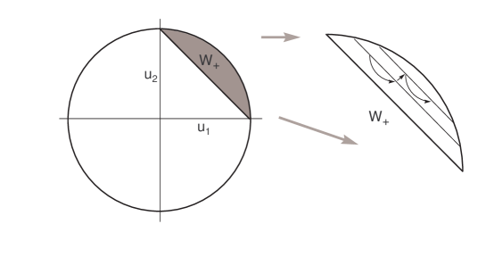
Figure 7. The region $W_{+}$ and the dynamics inside it.

We illustrate this process for $N=2$. Figure 7 shows $W_{+}$ in the $u_{1},u_{2}$ coordinates: $W_{+}$ is bounded by the circular arc $u_{1}^{2}+u_{2}^{2}=2$, $u_{1},u_{2}>0$, and its chord $u_{1}+u_{2}=\sqrt{2}$. Then $W_{+}$ is foliated by parallel lines $u_{1}+u_{2}=c$, $\sqrt{2}<c\leq 2$. The point $(u_{1},u_{2})$ stays on the same line $u_{1}+u_{2}=c$ at every collision between the disks and moves up to another line $u_{1}+u_{2}=c^{\prime}$ with $c^{\prime}>c$ during every collision with a wall.

Next we investigate the limit regime. Clearly there is a limit chord $u_{1}+u_{2}=c_{\infty}\leq 2$. If $c_{\infty}=2$, the chord degenerates to a single point $u_{1}=u_{2}=1$. In that case $v_{1}=v_{2}=0$, so the limit regime consists of both disks moving horizontally with the same unit speed.

If $c_{\infty}<2$, then the points $(u_{1},u_{2})$ along the trajectory of $X\in W_{+}$ accumulate on the chord $u_{1}+u_{2}=c_{\infty}$. We claim that they actually converge to one of the end points of that chord. Indeed, when the point $(u_{1},u_{2})$ is at a distance $\delta_{1}>0$ from the end points of the current chord $u_{1}+u_{2}=c$, then $u_{1}^{2}+u_{2}^{2}<2-\delta_{2}$ for some $\delta_{2}>0$ (which depends on $\delta_{1}$). Therefore $|v_{1}|>\delta_{3}$ or $|v_{2}|>\delta_{3}$ for some $\delta_{3}>0$ (which depends on $\delta_{2}$). Now we claim that at the next collision with a wall by one of the disks its vertical velocity will be $|v_{i}|>\delta_{4}$ for some $\delta_{4}>0$ (which depends on $\delta_{3}$). Indeed, a sequence of consecutive collisions between the two disks can be reduced to a simple billiard trajectory in a 2D periodic Lorentz gas [11, Section 4.2], and then one can easily check that the vertical components of their velocities cannot both vanish at the time they hit the walls.

Next, when a disk with a vertical velocity $|v_{i}|>\delta_{4}$ hits a wall, its velocity vector will be rotated so that $u_{i}$ will grow by some $\delta_{5}>0$ (which depends on $\delta_{4}$). Thus the point $(u_{1},u_{2})$ will move up to a chord $u_{1}+u_{2}=c+\delta_{6}$ for some $\delta_{6}>0$ (which depends on $\delta_{5}$). Hence the convergence to a limit chord can only occur when $(u_{1},u_{2})$ converges to one of its end points (and, as a result, $v_{1},v_{2}$ converge to zero).

In the above limit regime, when $c_{\infty}<2$, both disks move horizontally but at different speeds, $\bar{u}_{1}\neq\bar{u}_{2}$. We believe this actually happens with probability zero, but we can only give a heuristic argument. By Lemma 7.1 the disks have to collide from time to time. When they collide, their relative horizontal velocity is $u_{1}-u_{2}\approx\bar{u}_{1}-\bar{u}_{2}\neq 0$, but their relative vertical velocity is $v_{1}-v_{2}=\varepsilon\approx 0$. The collision of two disks can be reduced to a 2D periodic Lorentz gas with infinite horizon [11, Sect. 4.2].

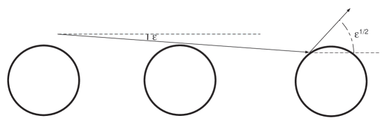
Figure 8. Nearly horizontal trajectories in a periodic Lorentz gas.

It is known in the studies of periodic Lorentz gases that if the vertical velocity of the moving particle before the collision is $\varepsilon$, then after the collision it is typically of order $\sqrt{\varepsilon}$, i.e., $v_{1}^{\prime}-v_{2}^{\prime}=\mathcal{O}(\sqrt{\varepsilon})$; see Figure 8. More precisely, there are $p,q>0$ such that the relative measure of initial conditions for which $v_{1}^{\prime}-v_{2}^{\prime}=\mathcal{O}(\varepsilon^{1/2-p})$ is $\mathcal{O}(\varepsilon^{q})$; see [31]. Thus in the course of infinitely many successive collisions between the disks their vertical velocities would explode sooner or later with probability one, violating the assumption $c_{\infty}<2$. This argument is not quite formal, as the word “probability” here refers to the canonical measure $\nu_{0}$, and in our dynamics the images of this measure keep changing, but we believe the conclusion is correct.

To summarize, we proved that in the limit regime the particles move horizontally to the right. We also conjecture that with probability one their horizontal velocities are equal:

(7.5) $$u_{1}=\cdots=u_{N}=1\qquad\text{and}\qquad v_{1}=\cdots=v_{N}=0.$$

In other words, almost all trajectories in $W_{+}$ converge to a limit regime where all the particles move horizontally and at unit speed. This is a stable limit regime, it corresponds to a submanifold $S_{+}$. This submanifold is defined by equations (7.5), hence its dimension is $2N$ (corresponding to the free coordinates $(x_{i},y_{i})$ of all the particles).

There is a symmetric region $W_{-}$ in phase space defined by

(7.6) $$W_{-}=\{u_{1}+\cdots+u_{N}<-\sqrt{N(N-1)}\},$$

where all the particles move in the negative $x$ direction. By a similar argument, almost all trajectories $X\in W_{-}$ converge to the stable limit regime where all the particles move horizontally to the left, and (we again conjecture) at unit speed:

(7.7) $$u_{1}=\cdots=u_{N}=-1\qquad\text{and}\qquad v_{1}=\cdots=v_{N}=0.$$

This corresponds to a submanifold $S_{-}$ of dimension $2N$.

Note that we have two stable limit regimes. Each one attracts a part of $\mathcal{M}$ that has a positive Lebesgue measure. Their basins of attraction are obviously disjoint, and due to symmetry they must have the same $\nu_{0}$-measure. Thus we have a coexistence of two attracting mechanisms in phase space.

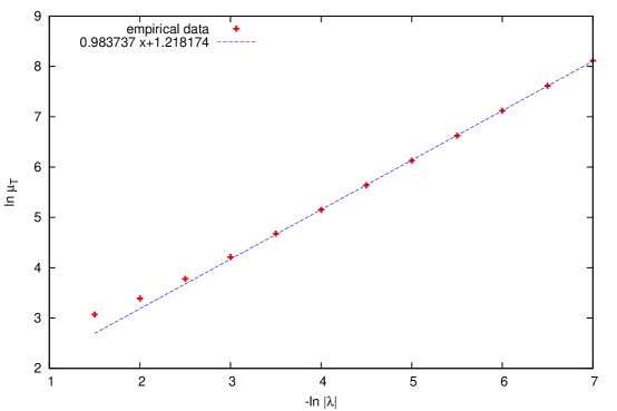
Figure 9. Plot of $\ln\mu_{\tau}$ versus $-\ln|\lambda|$. The least squares fit has slope of 0.983737.

Just like in Section 6 we estimated the escape time numerically. We used $N=2$ disks of diameter $d=0.1$ with the collision rules at the walls defined by (4.2)–(4.3) for various small $\lambda<0$. Figure 9 shows the mean escape time $\mu_{\tau}$ versus $\lambda$ on the log-log scale. The plot clearly demonstrates a linear pattern and the least square fitting line has slope 0.984 suggesting that $\mu_{\tau}\sim|\lambda|^{-1}$. Thus typical trajectories now escape much faster than in the case of stable center. We discuss the reason for the faster escape below.

Our main argument in Section 6 used the central limit theorem and was based on the chaotical character of the motion of the balls (before they enter the stable regime). However when the balls collide with the walls, our twisting rules (4.2)–(4.3) with $\lambda<0$ make the horizontal components of their velocities increase, thus the $x$ component of the total momentum, $u_{1}+u_{2}$, tends to grow (in absolute value). This tendency causes a drift toward larger values of $|u_{1}+u_{2}|$, i.e., toward the trapping regions $W_{\pm}$. Thus we should regard $u_{1}+u_{2}$ as a one-dimensional Itô diffusion process with a non-zero drift [18, 21].

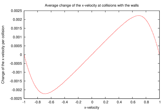
Figure 10. Average change of the $x$ component of the disks velocity $u$ versus its current value.

Figure 10 described the degree of the drift: it shows the average change of $u$, the $x$ component of the disk velocity, versus its current value (the plot was computed for $\lambda=-0.015$). We see that the absolute value $|u|$ always tends to increase, and this tendency is strong everywhere except when $u$ is close to 0 or $\pm 1$. In Section 6 we dealt with the balls that were approaching the hole $U_{0}$; then they moved nearly vertically, hence the drift was small and could be ignored. Now the balls are approaching the regions $W_{\pm}$; thus the drift is almost at its peak and its effect is crucial. Since the average drift, per collision, if of order $|\lambda|$, typical trajectories reach the regions $W_{\pm}$ of order $|\lambda|^{-1}$.

Figure 10 also shows that the drift persists as long as $|u|<1$, though it decreases as $|u|\to 1$. This supports our conjecture that typical trajectories converge to a limit regime where all the particles move at the same unit speed.

8. Generalizations

To summarize, the dynamics with unstable center ($\lambda<0$) is quite different from the one with stable center ($\lambda>0$). It has two distinct limit regimes ($S_{+}$ and $S_{-}$), both have dimension $2N$, while in the other case we had a single stable regime $S$ with dimension $3N-1$.

The attracting regions $W_{\pm}$ (“holes”) are of fixed size and measure (independent of $\lambda$), while for stable center the “hole” $U_{0}$ was quite narrow and had measure $\mathcal{O}(\lambda^{N})$.

Next we generalize our results. Our analysis of the stable center case applies to any stable fixed point of the map $g=f_{1}\circ f_{0}$ inside the interval $(0,\pi)$. Every such point produces a $T$-invariant open set $U_{0}\subset\mathcal{M}$, i.e., $T(U_{0})\subset U_{0}$, which acts as a “hole”. It has a basin of attraction in $\mathcal{M}$ of positive Lebesgue measure, and the limiting stable regime consists of disks moving with periodic incidence angles (assuming that the disks are small enough to avoid colliding with each other).

Of course if the map $g\colon[0,\pi]\to[0,\pi]$ has more than one stable fixed point, the corresponding basins of attraction are disjoint, so we have a coexistence of several attracting regimes.

Our analysis of the unstable center case applies to any map $g$ with stable fixed end points, 0 and $\pi$. In that case we have two attracting regimes similar to $S_{+}$ and $S_{-}$ above, and each has its own basin of attraction.

We must note that in the general case the “holes” $W_{\pm}$ need be defined more cautiously than (7.2) and (7.6). Precisely, we need to choose a small $\varepsilon_{0}>0$ and define $W_{\pm}$ by

$$W_{\pm}=\{\pm(u_{1}+\cdots+u_{N})>N-\varepsilon_{0}\}.$$

It is easy to verify that there is a $c=c(\varepsilon_{0})>0$ such that for every phase state in $W_{\pm}$ we have

$$\pm u_{i}>1-c\qquad\text{and}\qquad|v_{i}|<c$$

for all $i=1,\ldots,N$. Moreover, $c\to 0$ as $\varepsilon_{0}\to 0$. So we can choose, for example, $c=0.1$ and fix the corresponding $\varepsilon_{0}>0$ in the definition of $W_{\pm}$. Then of our analysis of the convergence to $S_{\pm}$ will not require significant changes.

In summary, every stable fixed point of the map $g\colon[0,\pi]\to[0,\pi]$ leads to a stable regime that attracts a set of positive Lebesgue measure in phase space.

In our numerical experiments, we mostly observed stable regimes for $N=2$ disks. Our analysis shows that they exist for larger $N$’s, too, but they become increasingly difficult to observe experimentally. Indeed, the sizes of the holes in phase space are exponentially small in $N$ (cf. (6.1), and a similar estimate can be derived for (7.2)), hence the escape time grows exponentially with $N$. Thus in physical systems with a large number of molecules the stable regimes become almost unobservable. Still, they exist for any $N$, and they dominate the dynamics for small $N$’s.

One may wonder whether attracting regimes exist when $g$ has no stable fixed points. For example, what if $g(\varphi)=\varphi$ is the identity map? The next section presents the most striking result: even in that case stable regimes may exist, which attract almost every phase trajectory!

9. Time reversible collisions with walls

Of special physical interest are twisting collisions (2.2) that make the dynamics time reversible. This means that if we reverse the velocity vectors of all our disks, then they will move along their past trajectories backwards. By direct inspection, the collision rule (2.2) is time reversible if and only if the function $f$ satisfies

(9.1) $$f\bigl{(}\pi-f(\varphi)\bigr{)}=\pi-\varphi.$$

This condition implies that the graph of the function $\psi=f(\varphi)$ is symmetric about the line $\psi=\pi-\varphi$.

If our collision rule is time reversible, i.e., satisfies (9.1), then we immediately arrive at $g(\varphi)=\varphi$.

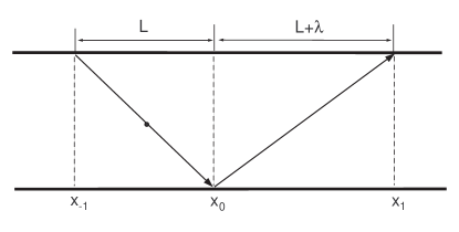
Figure 11. Collision rule pushing the particles to the right.

A simple example of a time-reversible rule is

(9.2) $$\cot f_{k}(\varphi)=(-1)^{k}\lambda+\cot\varphi$$

One can easily see that this definition is consistent with (2.3) and (9.1). The rule (9.2) can be written in the notation of (4.4) as

(9.3) $$u^{+}/|v^{+}|=u^{-}/|v^{-}|+(-1)^{k}\lambda.$$

This formula has a simple geometric interpretation: suppose a particle collides with a wall at a point with $x$-coordinate $x_{0}$, and we extend its trajectories before and after the collision until they cross the other wall at points whose $x$-coordinates we denote by $x_{-1}$ and $x_{1}$, respectively (see Figure 11), then

$$x_{1}-x_{0}=x_{0}-x_{-1}+(-1)^{k}\lambda.$$

If, for example, $\lambda>0$, then the above relation implies that the bottom wall $y=0$ pushes the particles to the right, and the top wall – to the left. This creates shear flow in the channel of the type studied in [7].

Next we describe a special regime in the above shear flow for $N=2$ disks. Suppose the disks move with opposite velocity vectors (i.e., their total momentum is zero) and they collide with opposite walls simultaneously. Then after the collision they again move with opposite velocity vectors.

When the disks collide with each other, then by symmetry their point of contact has coordinate $y=0.5$, i.e., the collision occurs right in the center of the channel. After the collision the disks move with opposite velocity vectors again, and will collide with the opposite walls simultaneously, etc. Hence this regime is invariant under our dynamics. See illustration in Figure 12.

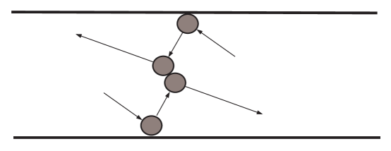
Figure 12. Special regime $S^{\ast}$ with symmetric motion.

We denote the above special family of phase trajectories by $S^{\ast}$. Note that dim$\,S^{\ast}=3$, while the (reduced) phase space is 6-dimensional, cf. Section 2.

A striking fact we discovered by numerical simulations is that the regime $S^{\ast}$ is stable and attracting. Almost every randomly selected phase trajectory eventually stabilizes near $S^{\ast}$ and then evolves in a symmetric fashion so that the disks move with opposite velocity vectors at equal distances from the opposite walls.

Actually, the regime $S^{\ast}$ may be also stable for the dynamics with an unstable center (Section 7), but this happens only for relatively large perturbations ($\lambda>0.6$). Since we are primarily interested in small perturbations, we will not discuss this last fact.

We provide a semi-heuristic argument showing that the regime $S^{\ast}$ is stable for the time-reversible collision rules, i.e., phase trajectories near $S^{\ast}$ tend to get closer to $S^{\ast}$ in the future.

We perturb the symmetries of the regime $S^{\ast}$ and show that perturbations tend to decrease, on average. There are two symmetries in the regime $S^{\ast}$: the velocity vectors of the disks are opposite, $\mathbf{v}$ and $-\mathbf{v}$, and their $y$-coordinates sum up to one, i.e., $y_{1}+y_{2}=1$.

First we perturb the velocity symmetry, i.e., suppose that the velocity vectors are $\mathbf{v}+\delta\mathbf{v}$ and $-\mathbf{v}$, i.e., the total momentum is a small $\delta\mathbf{v}\neq 0$. The interparticle collisions do not change the total momentum. When the disks collide with (opposite) walls, then the postcollisional velocity vectors will be denoted by $\mathbf{v}^{\prime}+\delta\mathbf{v}^{\prime}$ and $-\mathbf{v}^{\prime}$. Our goal is to show that $|\delta\mathbf{v}^{\prime}|$ tends to be smaller than $|\delta\mathbf{v}|$, on average.

We decompose $\delta\mathbf{v}=\delta\mathbf{v}_{\|}+\delta\mathbf{v}_{\perp}$ into the components parallel and perpendicular to $\mathbf{v}$, respectively. Similarly, $\delta\mathbf{v}^{\prime}=\delta\mathbf{v}_{\|}^{\prime}+\delta\mathbf{v}_{\perp}^{\prime}$ are the components of $\delta\mathbf{v}^{\prime}$ parallel and perpendicular to $\mathbf{v}^{\prime}$. Due to the conservation of the kinetic energy of each disk at the collision with the wall we have

$$|\mathbf{v}^{\prime}|=|\mathbf{v}|\qquad\text{and}\qquad|\mathbf{v}^{\prime}+\delta\mathbf{v}^{\prime}|=|\mathbf{v}+\delta\mathbf{v}|$$

hence

(9.4) $$|\delta\mathbf{v}_{\|}^{\prime}|=|\delta\mathbf{v}_{\|}|,$$

to the leading order. We will show that $|\delta\mathbf{v}_{\perp}^{\prime}|<|\delta\mathbf{v}_{\perp}|$, on average.

Let $\varphi$ and $\varphi+\delta\varphi$ denote the directional angles (i.e., angles made with the positive $x$ axis) of the velocity vectors $\mathbf{v}$ and $\mathbf{v}+\delta\mathbf{v}$, respectively. Let $\psi$ and $\psi+\delta\psi$ denote the directional angles of the velocity vectors $\mathbf{v}^{\prime}$ and $\mathbf{v}^{\prime}+\delta\mathbf{v}^{\prime}$, respectively. Then

$$\frac{|\delta\mathbf{v}_{\perp}|}{|\mathbf{v}|}=|\delta\varphi|\qquad\text{and}\qquad\frac{|\delta\mathbf{v}_{\perp}^{\prime}|}{|\mathbf{v}^{\prime}|}=|\delta\psi|$$

to the leading order, hence

(9.5) $$\frac{|\delta\mathbf{v}_{\perp}^{\prime}|}{|\delta\mathbf{v}_{\perp}|}=\frac{|\delta\psi|}{|\delta\varphi|}=|f_{k}^{\prime}(\varphi)|=f_{k}^{\prime}(\varphi)$$

(recall that $f_{k}$ is monotonically increasing, i.e., $f_{k}^{\prime}>0$).

Now after the collisions with the walls the particles move across the channel, and they either collide with each other or they miss each other and hit the opposite walls. In the latter case we denote by $\mathbf{v}^{\prime\prime}+\delta\mathbf{v}^{\prime\prime}$ and $-\mathbf{v}^{\prime\prime}$ their new postcollisional velocity vectors, and again decompose $\delta\mathbf{v}^{\prime\prime}=\delta\mathbf{v}_{\|}^{\prime\prime}+\delta\mathbf{v}_{\perp}^{\prime\prime}$. Then, inductively,

$$|\delta\mathbf{v}_{\|}^{\prime\prime}|=|\delta\mathbf{v}_{\|}^{\prime}|=|\delta\mathbf{v}_{\|}|$$

and

$$\frac{|\delta\mathbf{v}_{\perp}^{\prime\prime}|}{|\delta\mathbf{v}_{\perp}|}=\frac{|\delta\mathbf{v}_{\perp}^{\prime\prime}|}{|\delta\mathbf{v}_{\perp}^{\prime}|}\frac{|\delta\mathbf{v}_{\perp}^{\prime}|}{|\delta\mathbf{v}_{\perp}|}=f_{1-k}^{\prime}(\psi)f_{k}^{\prime}(\varphi)=g^{\prime}(\varphi)=1,$$

therefore $|\delta\mathbf{v}^{\prime\prime}|=|\delta\mathbf{v}|$.

We see that as long as the particles collide with the walls only, the perturbation vector $\delta\mathbf{v}$ changes periodically, with period two. So for an even number of wall collisions between two successive interparticle collisions, the net result will be zero change, i.e., $|\delta\mathbf{v}|$ will remain the same. For an odd number of wall collisions between two successive interparticle collisions, the net result will be the same as for just one wall collision, i.e., (9.5) will apply. Next we relate $|\delta\mathbf{v}_{\perp}|$ to $|\delta\mathbf{v}|$.

Consider an interparticle collision. It preserves the entire vector $\delta\mathbf{v}$, but the direction of the postcollisional velocity vector $\mathbf{v}$ can be regarded as a random variable uniformly distributed in the entire range $[0,2\pi]$, due to the scattering nature of the elastic collisions of hard disks. Let $\beta$ denote the directional angle of the vector $\delta\mathbf{v}$. Let $\varphi$ denote, as usual, the directional angle of the outgoing velocity vector $\mathbf{v}$. Then $|\delta\mathbf{v}_{\perp}|=|\delta\mathbf{v}|\,|\sin(\beta-\varphi)|$. The perturbation $\delta\mathbf{v}^{\prime}$ at the next interparticle collision will be

(9.6) $$|\delta\mathbf{v}^{\prime}|^{2}=|\delta\mathbf{v}|^{2}\bigl{(}\cos^{2}(\beta-\varphi)+\varkappa\sin^{2}(\beta-\varphi)\bigr{)}$$

where $\varkappa=[f_{k}^{\prime}]^{2}$ for an odd number of intermediate wall collisions and $\varkappa=1$ for an even number of intermediate wall collisions.

Next we estimate the total change of the norm $|\delta\mathbf{v}|$ over a long period of time $(0,T)$ during which $n$ interparticle collisions occur. We have $n-1$ intervals between successive interparticle collisions, and some of them (say, $m\leq n-1$ of them) have an odd number of collisions of each particle with the walls, while others (i.e., $n-m-1$ intervals) have an even number of collisions of each particle with the walls. Our previous analysis can be summarized as

(9.7) $$\log|\delta\mathbf{v}_{T}|-\log|\delta\mathbf{v}_{0}|=\tfrac{1}{2}\,\sum_{i=1}^{m}\log\bigl{[}1-\bigl{(}1-[f_{k_{i}}^{\prime}(\varphi_{i})]^{2}\bigr{)}\sin^{2}(\beta_{i}-\varphi_{i})\bigr{]},$$

where the summation is taken over the intervals with odd numbers of wall collisions.

Due to the randomization caused by the scattering effect of the interparticle collisions we can treat the angles $\beta_{i}$ and $\varphi_{i}$’s as independent random variables with uniform distribution in their ranges $0\leq\beta_{i}<2\pi$ and $0\leq\varphi_{i}\leq\pi$. We will prove in Appendix that the average value of each term in (9.7) is negative:

Lemma 9.1.

For both $k=0,1$ we have

$$\int_{0}^{\pi}\int_{0}^{2\pi}\log\bigl{[}1-\bigl{(}1-[f_{k}^{\prime}(\varphi)]^{2}\bigr{)}\sin^{2}(\beta-\varphi)\bigr{]}\,d\beta\,d\varphi=\mu_{1}<0.$$

Thus the sum in (9.7) approaches $-\infty$ linearly in $m$ (i.e., linearly in time), hence the norm of the perturbation $\delta\mathbf{v}$ decreases exponentially in time.

Second, we perturb the other symmetry of the regime $S^{\ast}$, i.e., we suppose that an interparticle collision occurs slightly above or below the central line $y=0.5$ of the channel. More precisely, let the point of contact at the moment of collision have coordinate $y=0.5+\ell$. At the same time we suppose that the particles have opposite velocity vectors, $\mathbf{v}=(u,v)$ and $-\mathbf{v}=(-u,-v)$, i.e., their total momentum is zero.

When the particles collide with the opposite walls, their postcollisional velocity vectors $(u^{\prime},v^{\prime})$ and $(-u^{\prime},-v^{\prime})$ will again be opposite. But the particles collide with the walls at slightly different moments of time, and the time interval between their collisions with the walls will be $2|\ell/v|$. If, after those collisions with the walls the particles collide with each other again, the point of contact will have coordinate $y=0.5+\ell^{\prime}$ with $|\ell^{\prime}|=|\ell v^{\prime}/v|$, i.e.,

(9.8) $$\log|\ell^{\prime}|-\log|\ell|=\log\bigl{(}|v^{\prime}|/|v|\bigr{)}=\log\bigl{(}\sin f(\varphi)/\sin\varphi\bigr{)}.$$

However, if the particles miss each other, then after their second collision with the opposite walls their velocities will be again $(u,v)$ and $(-u,-v)$. If the particles collide with each other after that, the point of contact will be again the distance $|\ell^{\prime}|=|\ell|$ from the central line $y=0.5$.

Thus the parity issue again arises and the formula (9.8) applies whenever the number of wall collisions between successive interparticle collisions is odd; otherwise there is no change, $|\ell^{\prime}|=|\ell|$. Thus, in the notation of (9.7) we have

(9.9) $$\log|\ell_{T}|-\log|\ell_{0}|\sim\sum_{i=1}^{m}\log\bigl{(}\sin f_{k_{i}}(\varphi_{i})/\sin\varphi_{i}\bigr{)}.$$

Again we treat $\varphi_{i}$’s as independent uniformly distributed random variables and verify that the mean value of $\log\bigl{(}\sin f(\varphi)/\sin\varphi\bigr{)}$ is negative. Proof of the following lemma will be given in Appendix.

Lemma 9.2.

For both $k=0,1$ we have

$$\frac{1}{\pi}\,\int_{0}^{\pi}\log\bigl{(}\sin f_{k}(\varphi)/\sin\varphi\bigr{)}\,d\varphi=\mu_{2}<0.$$

Thus the sum in (9.9) approaches $-\infty$ linearly in $m$ (i.e., linearly in time), hence the magnitude of the positional perturbation $\ell$ decreases exponentially in time.

This all verifies the stability of the regime $S^{\ast}$. Indeed, our perturbations by $\delta\mathbf{v}$ account for two directions transversal to $S^{\ast}$, and those by $\ell$ account for one more, hence we took care of all the three codimensions in the (reduced) 6-dimensional phase space.

We note that the classical (unperturbed) system of $N=2$ hard balls also leaves the manifold $S^{\ast}$ invariant. The dynamics within $S^{\ast}$ easily reduce to a periodic Lorentz gas with a single particle and infinite horizon. The periodic Lorentz gas is strongly hyperbolic and ergodic, thus the phase points $X\in S^{\ast}$ have one positive and one negative Lyapunov exponents, and typical phase trajectories within the manifold $S^{\ast}$ fill it densely. Interestingly, there are no expansion or contraction in any transversal direction to $S^{\ast}$, i.e., the points $X\in S^{\ast}$ have exactly one positive and one negative exponents with respect to the unperturbed dynamics in the entire phase space. This makes the manifold $S^{\ast}$ exceptional, as typical phase points are proven [23] to have two positive and two negative Lyapunov exponents, cf. Section 2.

We now describe what happens under our time-reversible perturbations. First, all the (previously zero) Lyapunov exponents in the directions transversal to $S^{\ast}$ seem to become negative, which instantly makes $S^{\ast}$ an attractor. (Here we refer to Lyapunov exponents of typical points $X\in S^{\ast}$.) Second, the (previously equivalent to the Lorentz gas) dynamics within $S^{\ast}$ is also perturbed, and it seems to retain its hyperbolic character and admit an SRB measure. For periodic Lorentz gases with infinite horizon under small perturbations the hyperbolicity is proven and a (unique) SRB measure is constructed in [12]. Perhaps the arguments of [12] could work in our case, too.

As a result, the SRB measure living on $S^{\ast}$ seems to attract nearly entire phase space. This makes it (the only) physically observable measure, as it describes the distribution of typical phase trajectories. Therefore, some kind of chaotic behavior does exist in the present case, but only after the six-dimensional phase space is reduced to the 3D surface $S^{\ast}$.

Lastly, we tried to find similar stable regimes for $N\geq 3$ balls with time-reversible twists at the walls, and did not observed any – the dynamics seem to be totally chaotic.

Acknowledgement. This work was motivated by discussions with J. Lebowitz and Ya. Sinai in March 2011, and we acknowledge the hospitality of Rutgers University and Princeton University. We thank D. Dolgopyat, J. Lebowitz, and A. Neishtadt for many useful remarks. N. C. is partially supported by NSF grant DMS-0969187. We are also grateful to the Alabama supercomputer administration for computational resources.

Appendix

First we prove Lemma 9.1. We note that $f_{k}^{\prime}(\varphi)>0$ and $\int_{0}^{\pi}f_{k}^{\prime}(\varphi)\,d\varphi=\pi$. With these assumptions the integral over $\beta$ can be taken analytically. It results in

$$\int_{0}^{2\pi}\log\left[1-\left(1-\left[f_{k}^{\prime}(\varphi)\right]^{2}\right)\sin^{2}(\beta-\varphi)\right]\,d\beta=4\pi\log\left[\frac{1}{2}\left(1+f_{k}^{\prime}(\varphi)\right)\right]$$

Now Jensen’s inequality works to show that

$$\frac{1}{\pi}\int_{0}^{\pi}\log\left[\frac{1}{2}\left(1+f_{k}^{\prime}(\varphi)\right)\right]\,d\varphi\leq\log\left[\frac{1}{\pi}\int_{0}^{\pi}\log\left[\frac{1}{2}\left(1+f_{k}^{\prime}(\varphi)\right)\right]\,d\varphi\right]=0$$

Lemma 9.1 is proved. ∎

Now we prove Lemma 9.2. Our arguments apply to both functions $f_{0}$ and $f_{1}$, so we suppress the index and denote them by $f$.

Recall that the graph of the function $\psi=f(\varphi)$ is symmetric about the line $\psi=\pi-\varphi$; see Figure 13. Thus it is convenient to use new variables

$$s=\frac{f(\varphi)+\varphi}{2}\qquad\text{and}\qquad w=\frac{f(\varphi)-\varphi}{2}.$$

If we drop a perpendicular from the point $(\varphi,f(\varphi))$, that lies on the graph, onto the main diagonal line $\psi=\varphi$, then its footpoint will be $(s,s)$, and its length will be $w\sqrt{2}$. The function $\psi=f(\varphi)$ becomes, in new variables, $w=w(s)$, and due to the above symmetry we have $w(\pi-s)=w(s)$, i.e., $w$ is an even function with respect to the center $s=\pi/2$. We also note that $w(0)=w(\pi)=0$, $|w^{\prime}|<1$, and

$$\varphi=s-w\qquad\text{and}\qquad f(\varphi)=s+w,$$

therefore

$$d\varphi=(1-w^{\prime})\,ds\qquad\text{and}\qquad\frac{df}{d\varphi}=\frac{df}{ds}\,\frac{ds}{d\varphi}=\frac{1+w^{\prime}}{1-w^{\prime}}.$$

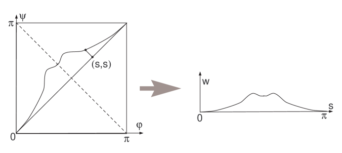
Figure 13. The graphs of $\psi=f(\varphi)$ and $w=w(s)$.

In these new variables the integral in Lemma 9.2 becomes

(9.10) $$\mu_{2}=\frac{1}{\pi}\,\int_{0}^{\pi}\log\frac{\sin(s+w)}{\sin(s-w)}(1-w^{\prime})\,ds$$

Note that

$$\int_{0}^{\pi}\log\frac{\sin(s+w)}{\sin(s-w)}\,ds=0$$

because of symmetry $w(\pi-s)=w(s)$.

We consider a function

(9.11) $$F(t):=\int_{0}^{\pi}\log\frac{\sin(s+tw)}{\sin(s-tw)}w^{\prime}\,ds$$

for $0\leq t\leq 1$. Note that $F(0)=0$. We will show that $F^{\prime}(t)>0$. Indeed,

$$2F^{\prime}(t) =\int_{0}^{\pi}\left(\cot(s+wt)+\cot(s-wt)\right)\,d(w^{2})$$

$$=\left.w^{2}\left(\cot(s+wt)+\cot(s-wt)\right)\right|_{0}^{\pi}$$

$$\;\;\;\;+\int_{0}^{\pi}\left(\frac{1+tw^{\prime}}{\sin^{2}(s+wt)}+\frac{1-tw^{\prime}}{\sin^{2}(s-wt)}\right)w^{2}\,ds$$

Recall that $w(0)=w(\pi)=0$ and $|w^{\prime}|<1$. This makes the middle line vanish. The integrand is always positive, which proves that $F^{\prime}(t)>0$. Then $F(t)>0$ for all $t>0$, and

$$\mu_{2}=-\tfrac{1}{\pi}\,F(1)<0\text{.}$$

Lemma 9.2 is proved. ∎

References

- [1] A. Arroyo, R. Markarian, D. P. Sanders, Bifurcations of periodic and chaotic attractors in pinball billiards with focusing boundaries, Nonlinearity 22 (2009) 1499–1522.
- [2] V. Baladi, C. Bonatti, and B. Schmitt, Abnormal escape rates from nonuniformly hyperbolic sets, Ergod. Th. Dynam. Syst. 19 (1999), 1111–1125.
- [3] H. van Beijeren, A. Latz, and J.R. Dorfman, Chaotic properties of dilute two- and three-dimensional random Lorentz gases II: Open systems, Phys. Rev. E 63 (2001), 016312.
- [4] W. Breymann, Z. Kovács, and T. Tél, Chaotic scattering in the presence of an external magnetic field, Phys. Rev. E 50 (1994), 1994-2006.
- [5] L. A. Bunimovich, C. Liverani, A. Pellegrinotti & Y. Suhov, Ergodic systems of balls in a billiard table, Comm. Math. Phys. 146 (1992), 357–396.
- [6] N. Chernov, G. Eyink, J. E. Lebowitz, and Ya. G. Sinai, Steady state electric conductivity in the periodic Lorentz gas, Comm. Math. Phys. 154 (1993), 569–601.
- [7] N. Chernov and J. Lebowitz, Stationary nonequilibrium states in boundary driven Hamiltonian systems: shear flow, J. Stat. Phys., 86 (1997), 953–990.
- [8] N. Chernov, Entropy, Lyapunov exponents and mean-free path for billiards, J. Stat. Phys., 88 (1997), 1–29.
- [9] N. Chernov, R. Markarian, and S. Troubetzkoy, Invariant measures for Anosov maps with small holes, Ergod. Th. Dynam. Syst. 20 (2000), 1007–1044.
- [10] N. Chernov, Sinai billiards under small external forces, Ann. H. Poincaré 2 (2001), 197–236.
- [11] N. Chernov and R. Markarian, Chaotic Billiards, Math. Surv. Monogr., 127, AMS, Providence, RI, 2006. (316 pp.)
- [12] N. Chernov and D. Dolgopyat, Anomalous current in periodic Lorentz gases with infinite horizon, Russ. Math. Surveys, 64 (2009), 73–124.
- [13] M. Demers, P. Wright, and L.-S. Young, Escape rates and physically relevant measures for billiards with small holes, Comm. Math. Phys. 294 (2010), 353–388.
- [14] G. Keller and C. Liverani, Rare Events, Escape Rates and Quasistationarity: Some Exact Formulae, J. Stat. Phys. 135 (2009), 519–534.
- [15] A. Krámli, N. Simányi & D. Szász, The K–property of three billiard balls, Ann. Math. 133 (1991), 37–72
- [16] A. Lopes and R. Markarian, Open Billiards: Invariant and Conditionally Invariant Probabilities on Cantor Sets, SIAM J. Appl. Math. 56 (1996), 651–680.
- [17] R. Markarian, E. J. Pujals, M. Sambarino, Pinball billiards with dominated splitting, Ergod. Th. Dynam. Syst. 30 (2010), 1757- 1786.
- [18] Oksendal B., Stochastic Differential Equations, Springer, Berlin, 2003.
- [19] E. Ott and T. Tél, Chaotic scattering: An introduction, Chaos 3 (1994), 417–426.
- [20] G. Pianigiani and J. Yorke, Expanding maps on sets which are almost invariant: decay and chaos, Trans. Amer. Math. Soc. 252 (1979), 351–366.
- [21] Revuz D. and Yor M. Continuous martingales and Brownian motion, 3d edition. Grundlehren der Mathematischen Wissenschaften, 293 (1999) Springer-Verlag, Berlin.
- [22] J. Schneider, T. Tél, and Z. NeufeldDynamics of leaking Hamiltonian systems, Phys. Rev. E. 66 (2002) 066218.
- [23] N. Simányi, Ergodicity of hard spheres in a box, Ergod. Th. Dynam. Syst. 19 (1999), 741–766.
- [24] N. Simányi, The complete hyperbolicity of cylindric billiards, Ergod. Th. Dyn. Sys. 22 (2002), 281–302.
- [25] N. Simányi, Proof of the Boltzmann-Sinai ergodic hypothesis for typical hard disk systems, Invent. Math. 154 (2003), 123–178.
- [26] N. Simányi, Proof of the ergodic hypothesis for typical hard ball systems, Ann. H. Poincaré 5 (2004), 203–233.
- [27] N. Simányi, Conditional proof of the Boltzmann-Sinai ergodic hypothesis (assuming the hyperbolicity of typical singular orbitz, Inventionnes 177 (2009), 381–413.
- [28] Ya. G. Sinai, On the foundations of the ergodic hypothesis for a dynamical system of statistical mechanics, Dokl. Akad. Nauk SSSR 153 (1963), 1261–1264.
- [29] Ya. G. Sinai, Dynamical systems with elastic reflections. Ergodic properties of dispersing billiards, Russ. Math. Surv. 25 (1970), 137–189.
- [30] D. Szász, Boltzmann’s Ergodic Hypothesis, a Conjecture for Centuries?, Studia Sci. Math. Hung. 31 (1996), 299–322.
- [31] Szasz D. and Varju T. Limit Laws and Recurrence for the Planar Lorentz Process with Infinite Horizon, J. Statist. Phys. 129 (2007), 59–80.
- [32] H. K. Zhang, Current in periodic Lorentz gases with twists, Comm. Math. Phys. 306 (2011), 747–776.