Critical properties of joint spin and Fortuin-Kasteleyn observables in the two-dimensional Potts model

Abstract

The two-dimensional Potts model can be studied either in terms of the original $Q$-component spins, or in the geometrical reformulation via Fortuin-Kasteleyn (FK) clusters. While the FK representation makes sense for arbitrary real values of $Q$ by construction, it was only shown very recently that the spin representation can be promoted to the same level of generality. In this paper we show how to define the Potts model in terms of observables that simultaneously keep track of the spin and FK degrees of freedom. This is first done algebraically in terms of a transfer matrix that couples three different representations of a partition algebra. Using this, one can study correlation functions involving any given number of propagating spin clusters with prescribed colours, each of which contains any given number of distinct FK clusters. For $0\leq Q\leq 4$ the corresponding critical exponents are all of the Kac form $h_{r,s}$, with integer indices $r,s$ that we determine exactly both in the bulk and in the boundary versions of the problem. In particular, we find that the set of points where an FK cluster touches the hull of its surrounding spin cluster has fractal dimension $d_{2,1}=2-2h_{2,1}$. If one constrains this set to points where the neighbouring spin cluster extends to infinity, we show that the dimension becomes $d_{1,3}=2-2h_{1,3}$. Our results are supported by extensive transfer matrix and Monte Carlo computations.

,

1 Introduction

The two-dimensional $Q$-state Potts model [1] is one of the most well-studied models in the realm of statistical physics. It can be addressed on the lattice using traditional approaches [2] (duality, series expansions, exact transformations) and algebraic techniques [3] (Temperley-Lieb algebra, quantum groups). In some cases it can be exactly solved using quantum inverse scattering methods [4]. When $0\leq Q\leq 4$ it gives rise to a critical theory in the continuum limit, which can in turn be investigated by the methods of field theory [5] (Coulomb gas, conformal field theory) or probability theory [6] (Stochastic Loewner Evolution). Despite of this well-equipped toolbox and sixty years of constant investigations, the Potts model remains at the forefront of current research, most recently in the context of logarithmic conformal field theory [7, 8].

The partition function of the Potts model reads

$$Z=\sum_{\sigma}\prod_{(ij)\in E}\exp\left(K\delta_{\sigma_{i},\sigma_{j}}\right)\,,$$ (1)

where $K$ is the coupling between spins $\sigma_{i}=1,2,\ldots,Q$ along the edges $E$ of some lattice ${\cal L}$. The Kronecker delta function $\delta_{\sigma_{i},\sigma_{j}}$ equals 1 if $\sigma_{i}=\sigma_{j}$, and 0 otherwise. The precise choice of ${\cal L}$ does not affect universal critical properties, so for convenience we choose the square lattice. The transition line—which gives rise to a critical theory for $0\leq Q\leq 4$—is then given by the selfduality criterion ${\rm e}^{K}=1+\sqrt{Q}$.

There are two obvious ways to rewrite the local Boltzmann weights:

$$\exp\left(K\delta_{\sigma_{i},\sigma_{j}}\right)=\left\{\begin{array}[]{ll}w\left[(1-\delta_{\sigma_{i},\sigma_{j}})w^{-1}+\delta_{\sigma_{i},\sigma_{j}}\right]\,,&w={\rm e}^{K}\,,\\ 1+v\delta_{\sigma_{i},\sigma_{j}}\,,&v={\rm e}^{K}-1\,,\end{array}\right.$$ (2)

where we have used that $\delta_{\sigma_{i},\sigma_{j}}=0$ or $1$. The partition function (1) is obtained by expanding a product of such factors; each term in the expansion corresponds to choosing, for each $(ij)\in E$, either the first or the second term in (2).

Consider first the expansion in powers of $w^{-1}$. Each factor of $w^{-1}$ comes with the term $(1-\delta_{\sigma_{i},\sigma_{j}})$ that forces the spins $\sigma_{i}$ and $\sigma_{j}$ to take different values; there is thus a piece of domain wall (DW) on the edge $(ij)^{*}$ dual to $(ij)$. Making this choice for each $(ij)\in E$ defines a DW configuration on the dual lattice ${\cal L}^{*}$. This DW configuration defines a graph $G$ (not necessarily connected), the faces of which are the clusters of aligned spins. Since we do not specify the colour of each of these clusters, a DW configuration has to be weighted by the chromatic polynomial $\chi_{G^{*}}(Q)$ of the dual graph $G^{*}$. Initially $\chi_{G^{*}}(Q)$ is defined as the number of colourings of the vertices of the graph $G^{*}$, using colours $\{1,2,\ldots,Q\}$, with the constraint that neighbouring vertices have different colours. This is indeed a polynomial in $Q$ for any $G$, and so can be evaluated for any real $Q$ (but $\chi_{G^{*}}(Q)$ is integer only when $Q$ is integer). The partition function (1) can thus be written as a sum over all possible DW configurations

$$Z_{\rm spin}=w^{N}\sum_{G}\,w^{-{\rm length}(G)}\,\chi_{G^{*}}(Q)\,,$$ (3)

where $N$ is the number of spins, and ${\rm length}(G)$ denotes the total length of the domain walls.

Alternatively we may consider the expansion in powers of $v$. The set of edges $(ij)\in E$ for which the term $v\delta_{\sigma_{i},\sigma_{j}}$ is chosen defines a graph $H$, the connected components of which are known as Fortuin-Kasteleyn (FK) clusters [9]. Since spins belonging to the same FK cluster are obviously aligned, we can perform the sum over $\{\sigma_{i}\}$ in (1) to obtain

$$Z_{\rm FK}=\sum_{H}Q^{{\rm\sharp clusters}(H)}v^{{\rm\sharp edges}(H)}\,.$$ (4)

We stress that spins belonging to different FK clusters can still be aligned (with probability $1/Q$), even if the two clusters are adjacent on the lattice.

Despite of the fact that $Z_{\rm spin}=Z_{\rm FK}=Z$ exactly, the different geometrical degrees of freedom ($G$ resp. $H$) underlying the spin and FK formulations give rise to different critical exponents in the continuum limit for $0\leq Q\leq 4$. In both cases it is possible to build $Z$ from a transfer matrix that acts on respectively the FK [10] and spin [11] degrees of freedom. The transfer matrix is an essential ingredient in both analytical and numerical studies, and it gives access to the rich algebraic structures underlying the Potts model. In the FK case this structure is the Temperley-Lieb algebra [3], whereas the particular partition algebra that emerges in the spin case [11] still awaits a complete study.

Critical exponents corresponding to FK clusters were first derived by Coulomb gas techniques (see e.g. [5]) and have subsequently been confirmed by the rigorous methods of SLE (see e.g. [6]). In particular the probability that $\ell$ distinct FK clusters propagate between small neighbourhoods of two distant points defines a critical exponent that can be found in the Kac table of CFT as $h_{0,\ell}$ in the bulk case, and as $h_{1,1+2\ell}$ in the boundary case [12]. The spin case turns out to be richer, since one needs in addition to specify the respective colours of the propagating spin clusters. A pair of adjacent clusters having different (resp. identical) colours give rise to a thin (resp. a thick) DW. The exponents corresponding to $\ell_{1}$ thin DW and $\ell_{2}$ thick DW can be identified as $h_{\ell_{1}-\ell_{2},2\ell_{1}}$ in the bulk case and as $h_{1+2(\ell_{1}-\ell_{2}),1+4\ell_{1}}$ in the boundary case [11]. At present this result is based on (substantial) numerical evidence, supported by analytical arguments for the special case $\ell_{1}=0$.

The purpose of this paper is to study the joint properties of FK and spin clusters, by simultaneously keeping track of the geometrical degrees of freedom $G$ and $H$ appearing in (3)–(4). The corresponding geometrical observables are defined precisely in section 2. We show that making certain physical assumptions—and insisting on recovering the results for FK [12] and spin [11] clusters as special cases—leads to a conjecture for the scaling dimensions of joint observables in the general case. This conjecture generalises all the preceeding results and gives access to new information on the interaction between FK and spin clusters. All the scaling dimensions fit into the Kac table $h_{r,s}$ with integer indices $r$ and $s$.

This result constitutes a further step in the programme [13] of classifying non-unitary boundary conditions in two-dimensional geometrical models.

In section 3 we define a transfer matrix that contains complete information about these joint spin-FK observables. It formally acts on three coupled partition algebras. We study its spectrum numerically in section 4, finding strong support for our general conjecture for the scaling dimensions of geometrical observables. In section 5 we further corroborate the conjecture by studying the most relevant among the new exponents by Monte Carlo simulations. We discuss our findings in section 6.

2 Joint spin and FK observables

We begin by reviewing the definition of observables in the spin representation of the Potts model [11]. For the purposes of this discussion it suffices to consider two-point correlation functions. We then ask how the probability, that a certain number $\ell$ of spin clusters—each corresponding to a given value of the spin $\sigma_{i}$—connect a small (in units of the lattice spacing) neighbourhood $A$ to another small neighbourhood $B$, decays when the distance $x$ between $A$ and $B$ increases. It is convenient to specify the two-point function by just giving the $\ell$ colour labels $\sigma_{i}$. By the $S_{Q}$ permutation symmetry only the relative colours matter. For instance, with $\ell=4$ the labels $1123$ and $2241$ specify the same correlation function.

Alternatively one may think of this question in terms of the DW that separate pairs of adjacent (when moving along the rim of $A$ or $B$) spin clusters. Each DW can be either thin or thick, depending on whether the two adjacent clusters have different or identical colours. The reason for this nomenclature is that adjacent spin clusters with different colours can touch (in which case the corresponding DW has a width of one lattice spacing), whereas if the colours are identical they cannot (since then there would be no separating DW). In other words, the width of a thick DW is at least two lattice spacings. The results of [11] show that this distinction is important, since it survives in the continuum limit and gives rise to different critical exponents.

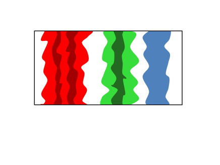
Figure 1: Schematic example of excitations considered in this paper, with three spin clusters carrying different coulours propagating along the imaginary time direction. The shaded regions represent propagating FK clusters living inside the spin clusters. Using the notations (5), this excitation corresponds to $1^{2}2^{1}3^{0}$.

An obvious but important consequence of (2) is that if two points belong to the same FK cluster, it implies that they also belong to the same spin cluster. The opposite implication is however not true. This means that FK clusters live “inside” spin clusters, and in particular a given spin cluster can contain several distinct FK clusters. This suggests introducing a more general two-point function where each propagating spin cluster contains a given non-negative number of propagating FK clusters. We describe this by a label

$$\sigma_{1}^{\alpha_{1}}\sigma_{2}^{\alpha_{2}}\ldots\sigma_{\ell}^{\alpha_{\ell}}\,,$$ (5)

where $\sigma_{k}$ is the colour of $k$’th spin cluster, and $\alpha_{k}=0,1,2,\ldots$ is the number of FK clusters living inside the $k$’th spin cluster. An example of such an excitation is shown in Fig. 1.

2.1 Result for bulk and boundary critical exponents

Two different geometries are of interest. In the bulk case, the neighbourhoods $A$ and $B$ are at arbitrary, but widely separated, locations in the infinite plane. This is conformally equivalent to an infinitely long cylinder—a strip with periodic boundary conditions—with $A$ and $B$ situated at the two extremities. In the boundary case, the geometry is that of the upper half plane, with $A$ being at the origin and $B$ far away from the real axis. It suffices to consider free boundary conditions on the real axis, since the work of [11] has already demonstrated that fixed or mixed boundary conditions on the positive real axis can be accommodated by fusing the operator that inserts the propagating (spin and FK) clusters with an appropriate boundary condition changing operator at the origin.

The results for the critical exponents can be stated in terms of the Kac parametrisation of CFT

$$h_{r,s}=\frac{\left(r-s\,\kappa/4\right)^{2}-\left(1-\kappa/4\right)^{2}}{\kappa}\,,$$ (6)

where $2\leq\kappa\leq 4$ parameterises the number of states $Q\in[0,4]$ via

$$Q=4\left(\cos\frac{\kappa\,\pi}{4}\right)^{2}\,.$$ (7)

In the bulk case (geometry of the plane) the critical exponent corresponding to the two-point function defined above is denoted $h(Q)=h(Q;\sigma_{1}^{\alpha_{1}}\sigma_{2}^{\alpha_{2}}\ldots\sigma_{\ell}^{\alpha_{\ell}})$, and the correlation function (or probability) of the prescribed event decays like $P\propto x^{-4h(Q)}$ for $x\gg 1$. Equivalently, on a long cylinder of size $L\times M$ with $M\gg L$, periodic boundary conditions in the $L$-direction, and $A$ and $B$ identified with the opposite ends of the cylinder, the decay is exponential: $P\propto{\rm e}^{-4\pi(M/L)\,h(Q)}$. In the boundary case (geometry of the half plane) the critical exponent for free boundary conditions is denoted $\widetilde{h}(Q)$.

We can write the bulk and boundary exponents in a unified way as

$$h(Q) = h_{q_{1},q_{2}}\,,$$ (8)

$$\widetilde{h}(Q) = h_{1+2q_{1},1+2q_{2}}\,,$$ (9)

where the right-hand side refers to (6) and we have defined a “charge” $(q_{1},q_{2})$. The result of [12] is then that $\ell$ propagating FK clusters correspond to

$$(q_{1},q_{2})=(0,\ell)\,,\qquad\qquad\ \ \ \mbox{for FK clusters.}$$ (10)

In the case of spin clusters with $\ell_{1}$ thin DW and $\ell_{2}$ thick DW the result of [11] is that

$$(q_{1},q_{2})=(\ell_{1}-\ell_{2},2\ell_{1})\,,\qquad\mbox{for spin clusters.}$$ (11)

These results strongly suggest that the costs for creating an excitation consisting of several types of interfaces simply add up at the level of the charge $(q_{1},q_{2})$. This is a well-known situation in the Coulomb gas (CG) formalism. But note that whereas the result (10) for FK clusters indeed admits a CG derivation [12] no such argument has yet been established for the spin cluster result (11). Admitting the additivity of charges, we can nevertheless read off the following rules from (11)

$$(q_{1},q_{2})=\left\{\begin{array}[]{ll}(1,2)&\mbox{for a thin DW}\,,\\ (-1,0)&\mbox{for a thick DW}\,.\end{array}\right.$$ (12)

We now argue that two additional rules are needed for dealing with the insertion of FK clusters inside a given spin cluster. Indeed, when a single FK cluster is inserted ($\alpha_{i}=1$) we create a pair of interfaces separating the hull of the FK cluster from the hull of the surrounding spin cluster. The insertion of each subsequent FK cluster (when $\alpha_{i}>1$) will in addition create an interface separating the FK cluster from the one preceeding it. To match (10) we clearly need $(q_{1},q_{2})=(0,1)$ in the latter case. To deal with the former, we note that using our conventions, a configuration with just $\ell$ FK clusters can either be labelled $1^{\ell}$ (if each FK cluster has the same colour) or $1^{1}2^{1}\ldots\ell^{1}$ (if each FK cluster has a different colour). In either case, additivity of charges and consistency with (10) requires the correct rule to be

$$(q_{1},q_{2})=\left\{\begin{array}[]{ll}(-1,-1)&\mbox{for the first FK in a given spin cluster}\,,\\ (0,1)&\mbox{for each subsequent FK in that cluster}\,.\end{array}\right.$$ (13)

The main result of this paper is the following conjecture:

• Consider the excitation labelled as in (5). Compute the corresponding charge $(q_{1},q_{2})$ by adding up the contributions from the $\sigma_{k}$, using rules (12), and those of the $\alpha_{k}$, using rules (13). Then the bulk and boundary critical exponents are given by (8)–(9).

2.2 Remarks on the first spin cluster

The reader will have noticed that the nature (thin or thick) of the DW are determined by the relative colours of two spin clusters. It therefore remains to discuss carefully how to account for the first one of the spin clusters making up the excitation.

In the bulk case, when only a single spin cluster is present ($\ell=1$), it will almost surely wrap around the periodic direction (i.e., separate the neighbourhoods $A$ and $B$). Our results do not apply to this case. Indeed, it is well known that the critical exponent in this case is the magnetic exponent $h_{1/2,0}$ (resp. $h_{0,\alpha_{1}}$) for a spin cluster with $\alpha_{1}=0$ (resp. $\alpha_{1}\geq 1$) propagating FK clusters, cf. (10). If, on the other hand, we impose the additional constraint that the spin cluster must not wrap around the periodic direction, our results do apply. The constraint then amounts to the presence of one thick DW that separates the spin cluster from itself.

In the boundary case, our results always apply, provided that the first spin cluster is counted as a thin DW. This makes intuitive sense, since the free boundary conditions permit the spin cluster to touch the boundary, just as in the case of two spins clusters with different colours.

2.3 Possible values of the exponents $h_{r,s}$

It is obvious that all excitations of the type (5) will lead to charges $(q_{1},q_{2})$, where $q_{1}$ and $q_{2}$ take integer (positive or negative) values. We now wish to clarify precisely which values $(q_{1},q_{2})\in\mathbb{Z}^{2}$ can be obtained through the joint spin-FK observables.

The spin part of the excitation is described by the numbers $(\ell_{1},\ell_{2})$ of thin and thick DWs, as in (11). We first discuss the boundary case, for which the allowed values are $\ell_{1}\geq 1$ (since the first DW is thin) and $\ell_{2}\geq 0$. Using rules (12)–(13) one can then deduce the possible values of the charge $(q_{1},q_{2})$:

• For $q_{1}\geq 1$, we have the constraint $q_{2}\geq 2q_{1}$. Indeed, the excitation with $(\ell_{1},\ell_{2})=(q_{1},0)$ and no FK clusters gives the charge $(q_{1},2q_{1})$, while the one with $(\ell_{1},\ell_{2})=(q_{1}+1,0)$ and a single FK cluster on one of the spin clusters gives the charge $(q_{1},2q_{1}+1)$. Any higher value of $q_{2}$ can be attained by placing additional FK clusters on the same spin cluster.

• For even $q_{1}\leq 0$, we have the constraint $q_{2}\geq\frac{q_{1}+2}{2}$. Indeed, the excitation with $(\ell_{1},\ell_{2})=(1,-\frac{q_{1}}{2})$ and one FK cluster on each one of the spin clusters corresponds to $q_{2}=\frac{q_{1}+2}{2}$, while any higher value can be obtained by adding further FK clusters.

• For odd $q_{1}\leq 0$, we have the constraint $q_{2}\geq\frac{q_{1}+3}{2}$. Indeed, the excitation with $(\ell_{1},\ell_{2})=(1,-\frac{q_{1}-1}{2})$ and one FK cluster on each of the spin clusters except the first one saturates the inequality on $q_{2}$, whose value can be increased by the addition of more FK clusters.

The discussion of the bulk case is similar, except that the allowed values of $(\ell_{1},\ell_{2})$ are $\ell_{1},\ell_{2}\geq 0$ with $\ell_{1}\neq 1$ (because of the periodic boundary conditions), and of course $(\ell_{1},\ell_{2})\neq(0,0)$ in order to have a non-trivial excitation. The leads only to a very minor modification of the constraints on the charge $(q_{1},q_{2})$ derived in the boundary case: For $q_{1}<0$ we have now $q_{2}\geq\lceil\frac{q_{1}}{2}\rceil$.

In conclusion, the spin-FK observables described in this paper make it possible to produce (say, in the bulk case) all the Kac table exponents $h_{r,s}$ with integer indices $(r,s)$ above or below both of the lines $s=2r$ and $s=r/2$. The two cones in between these lines are not accessible by the spin-FK observables.

3 Transfer matrix construction

We now describe a transfer matrix whose spectrum contains all of the excitations discussed in section 2.

First recall that a partition ${\cal P}$ of a set $X$ is a set of nonempty subsets of $X$ such that every element $i\in X$ is in exactly one of these subsets. The elements of ${\cal P}$ (i.e., the nonempty subset of $X$) are called blocks. A block containing precisely one element of $X$ is called a singleton. A partition ${\cal P}_{a}$ is said to be a refinement of ${\cal P}_{b}$, and we write ${\cal P}_{a}\preceq{\cal P}_{b}$, provided that each block in ${\cal P}_{a}$ is a subset of some block in ${\cal P}_{b}$. This defines a partial order of the partitions of $X$.

We shall need a few simple operators acting on ${\cal P}$. We denote the identity operator by $I$. For $i,j\in X$ the join operator $J_{ij}$ acts as $I$ if $i$ and $j$ belong to the same block; if not, it amalgamates the block containing $i$ with the block containing $j$ so as to form a single block. The detach operator $D_{i}$ acts by detaching $i$ from its block, i.e., by transforming it into a new singleton block $\{i\}$.

If we associate a Potts spin $\sigma_{i}$ with each $i\in X$ we can finally define the indicator operator as $\Delta_{ij}=\delta_{\sigma_{i},\sigma_{j}}\cdot I$.

In the representation theory of the Temperley-Lieb algebra, $D_{i}$ is usually defined in a slightly different manner. Namely, $D_{i}$ acts as $\widetilde{Q}\cdot I$ if $i$ is a singleton (i.e., it gives a Boltzmann weight $\widetilde{Q}$); otherwise it transforms $i$ into a singleton (with a Boltzmann weight $1$). Then, setting $e_{2i-1}=\widetilde{Q}^{-1/2}D_{i}$ and $e_{2i}=\widetilde{Q}^{1/2}J_{i,i+1}$, the $e_{k}$ provide a representation of the Temperley-Lieb algebra [3] corresponding to the $\widetilde{Q}$-state Potts model. In our construction of the transfer matrix we shall account for $Q$ in a different manner, which is why we have set $\widetilde{Q}=1$ above.

3.1 States and elementary transfer matrices

The states of the Potts model in the spin-FK representation are given by a triplet of partitions $({\cal P}_{1},{\cal P}_{2},{\cal P}_{3})$ of the set $X$ of vertices within a row of the lattice ${\cal L}$.

The first partition ${\cal P}_{1}$ is arbitrary (not necessarily planar) and describes the spin colours: we have $\sigma_{i}=\sigma_{j}$ if and only if $i,j$ belong to the same block in ${\cal P}_{1}$. The second partition ${\cal P}_{2}$ is planar and describes the connectivity of spin clusters. We have ${\cal P}_{2}\preceq{\cal P}_{1}$, since spins in the same spin cluster have equal colours. The third partition ${\cal P}_{3}$ is again planar and describes the connectivity of FK clusters. We have ${\cal P}_{3}\preceq{\cal P}_{2}$, since spins in the same FK cluster are also in the same spin cluster.

We represent graphically the transfer matrix as

(14)

The elementary transfer matrix $T_{\rm h}$ that adds a horizontal edge between vertices $i$ and $j$ acts in ${\cal P}_{1}\otimes{\cal P}_{2}\otimes{\cal P}_{3}$ as follows:

$$T_{\rm h}=1\cdot(I-\Delta_{ij})\otimes I\otimes I+({\rm e}^{K}-1)\cdot\Delta_{ij}\otimes J_{ij}\otimes J_{ij}+1\cdot\Delta_{ij}\otimes J_{ij}\otimes I\,,$$ (15)

where the number before the dot ($\cdot$) is the Boltzmann weight. The first term corresponds to the two spins $\sigma_{i}$ and $\sigma_{j}$ being different, in which case $i,j$ can neither be in the same spin cluster, nor in the same FK cluster. The second term corresponds to $i,j$ being in the same FK cluster, hence also in the same spin cluster. Finally, the third term corresponds to $i,j$ having the same spin without being in the same FK cluster; in this case the spin clusters must be joined up since $i,j$ are neighbours on the lattice.

We can similarly define the elementary transfer matrix $T_{\rm v}$ that adds a vertical edge edge to the lattice, by propagating the vertex $i$ to a new vertex $i^{\prime}$. It acts in ${\cal P}_{1}\otimes{\cal P}_{2}\otimes{\cal P}_{3}$ like

$$T_{\rm v}=1\cdot(I-\Delta_{ii^{\prime}})\otimes D_{i}\otimes D_{i}+({\rm e}^{K}-1)\cdot\Delta_{ii^{\prime}}\otimes I\otimes I+1\cdot\Delta_{ii^{\prime}}\otimes I\otimes D_{i}\,,$$ (16)

and each term has the same interpretation as in $T_{\rm h}$. Since $T$ builds up the partition function $Z$, it must also account for the summation $\sum_{\sigma}$ over the spin varibles, cf. (1). The easiest convention is to let the action of $T_{\rm v}$ be accompanied by a sum over $\sigma_{i^{\prime}}$. This sum is dealt with in the same way as in [11]. Namely, let $\Sigma$ denote the set of spin values $\{\sigma_{i}\}$ being used in a given state, so that the number of elements $|\Sigma|$ is just the number of blocks in ${\cal P}_{1}$. After summing over $\sigma_{i^{\prime}}$, the second and third terms in (16) each correspond to a single non-zero contribution. The first term gives $|\Sigma|-1$ contributions where $\sigma_{i^{\prime}}\neq\sigma_{i}$, but $\sigma_{i^{\prime}}\in\Sigma$. The remaining contributions, where $\sigma_{i^{\prime}}\neq\sigma_{i}$ and $\sigma_{i^{\prime}}\notin\Sigma$ can be regrouped (using the overall $S_{Q}$ symmetry) as a single contribution, with Boltzmann weight $Q-|\Sigma|$, in which $\{i^{\prime}\}$ becomes a singleton in ${\cal P}^{\prime}_{1}$. It is precisely because of this regrouping that it now makes sense to promote $Q$ to an arbitrary real variable [11].

The complete row-to-row transfer matrix $T$ for a system of size $L$, shown graphically in (14), is then obtained as the product of the elementary transfer matrices corresponding to all horizontal and vertical edges in a row:

$$T=\left(\prod_{i=1}^{L}T_{\rm v}^{(i)}\right)\times\left(\prod_{i=1}^{L^{\prime}}T_{\rm h}^{(i,i+1)}\right)\,,$$ (17)

where $L^{\prime}=L-1$ in the boundary case (strip geometry) and $L^{\prime}=L$ with indices $i$ considered modulo $L$ in the bulk case (cylinder geometry).

Several remarks are in order:

1. When representing ${\cal P}_{1}$ one can replace the actual spin values $\sigma_{i}$ by colour labels $c_{i}$ defined such that $c_{i}=c_{j}$ if and only if $\sigma_{i}=\sigma_{j}$. Using the $S_{Q}$ symmetry these colour labels can be brought into a standard form, thus reducing the number of basis states. Details of this construction are given in [11].

2. For a system of size $L$, at most $L$ different colour labels are used. Therefore the number of basis states depends only on $L$, and not on $Q$. In particular the state space is finite.

3. The three partition algebras ${\cal P}_{1}$, ${\cal P}_{2}$ and ${\cal P}_{3}$ are coupled by virtue of (15)–(16). It is an interesting problem, beyond the scope of this paper, to analyse in details this situation from a representation theoretical point of view.

4. If one neglects the information on FK clusters contained in ${\cal P}_{3}$, the second and third terms in (15)–(16) can be resummed, and one recovers the construction of [11].

5. If one neglects the information on spin clusters contained in ${\cal P}_{2}$, the first and third terms in (15)–(16) can be resummed. The result is then independent of ${\cal P}_{1}$ and reproduces the well-known Temperley-Lieb representation [3].

6. In the above construction we have accounted for $Q$ in the partition algebra ${\cal P}_{1}$. Therefore, the detach operators $D_{i}$ acting on ${\cal P}_{2}$ and ${\cal P}_{3}$ have parameter $\widetilde{Q}=1$. In particular, the FK clusters described by ${\cal P}_{3}$ can be thought of as percolation ($\widetilde{Q}=1$) clusters inside the spin clusters described by ${\cal P}_{1}$ and ${\cal P}_{2}$. Leaving $\widetilde{Q}$ as a free parameter would amount to studying FK clusters of a second $\widetilde{Q}$-state Potts model defined on top of the spin clusters of the original $Q$-state Potts model. This appears to be an interesting way of coupling a pair of $(Q,\widetilde{Q})$-state Potts models—and we intend to report further on this elsewhere.

The leading eigenvalue $\Lambda_{0}$ of the transfer matrix $T$ gives the ground state free energy $f_{0}=-\frac{1}{L}\log\Lambda_{0}$. This $f_{0}$ coincides precisely with that of the usual FK transfer matrix [10], even when $Q$ is non-integer. Its finite-size corrections possess a universal $L^{-2}$ term whose coefficient determines the central charge of the corresponding CFT [14].

3.2 Correlation functions

To obtain the two-point correlation defined in section 2 we need a variant transfer matrix $T^{\prime}$ which imposes the propagation of the defect labelled as in (5) along the (imaginary) time direction of the cylinder (or strip). From its leading eigenvalue $\Lambda^{\prime}_{0}$ one can determine the energy gap $\Delta f=-\frac{1}{L}\log(\Lambda^{\prime}_{0}/\Lambda_{0})$ whose finite-size scaling in turn determines the critical exponents $h(Q)$ and $\widetilde{h}(Q)$ [14, 5].

To construct $T^{\prime}$ we modify the basis states ${\cal P}_{1}\otimes{\cal P}_{2}\otimes{\cal P}_{3}$ by marking some of the blocks in the partitions ${\cal P}_{2}$ and ${\cal P}_{3}$. First, we mark $\ell$ blocks in ${\cal P}_{2}$ whose spin colours in ${\cal P}_{1}$ coincide with the choice of $\{\sigma_{1},\sigma_{2},\ldots,\sigma_{\ell}\}$ in (5). Second, let ${\cal P}_{3}$ be a refinement of ${\cal P}_{2}$ such that the $k$’th marked block in ${\cal P}_{2}$ is refined into at least $\alpha_{k}$ blocks in ${\cal P}_{3}$, of which precisely $\alpha_{k}$ are marked.

In order to conserve the marked clusters in the transfer matrix evolution, none of the marked clusters must be “left behind”, and two distinct marked clusters must not be allowed to link up. Imposing these rules in a precise way is tantamount to defining a modified action of the join and detach operators, $J_{ij}$ and $D_{i}$, on the marked basis states. Namely, $J_{ij}$ is modified to give a zero Boltzmann weight if $i,j$ are in distinct marked blocks (this prevents a marked block from disappearing), and $D_{i}$ is modified to give a zero Boltzmann weight if $\{i\}$ is a marked singleton block (this prevents marked blocks from being “left behind”). Finally, when $J_{ij}$ joins a marked and an unmarked block, the result is a marked block.

The full state space corresponding to the excitation (5) is generated by letting $T^{\prime}$ act a sufficient number of times on a suitable initial basis state. This initial state is such that the $k$’th marked block in ${\cal P}_{2}$ consists of $\alpha_{k}$ consecutive points $\{i_{k},i_{k}+1,\ldots,i_{k}+\alpha_{k}-1\}$ in a row of the lattice. In the refining partition ${\cal P}_{3}$ each of these $\alpha_{k}$ points is a marked singleton. Finally, those of the $L$ points which are not marked in this construction of the initial state are taken as singletons, both in ${\cal P}_{2}$ and in ${\cal P}_{3}$.

In summary, the modified transfer matrix $T^{\prime}$ keeps enough information, both about the mutual colouring of the sites and about the connectivity of spin and FK clusters, to give the correct Boltzmann weights to the different configurations, even for non-integer $Q$, and to follow the time evolution of the excitation defined by (5).

4 Exact diagonalisation results

We have numerically diagonalised the transfer matrix in the spin-DW representation for cylinders (resp. strips) of width up to $L=8$ (resp. $L=9$) spins. We verified that the leading eigenvalue $\Lambda_{0}$ in the ground state sector coincides with that of the FK transfer matrix, including for non-integer $Q$. As to the excitations $\Lambda^{\prime}_{0}$, we explored systematically all possible colouring combinations (5) for up to $\ell=3$ marked spin clusters with different choices for the number of FK clusters $\alpha_{k}$, for a variety of values of the parameter $\kappa$.

Finite-size approximations of the critical exponents $h(L)$ and $\widetilde{h}(L)$ were extracted from the leading eigenvalue in each sector, using standard CFT results [14, 5], and fitting both for the universal corrections in $L^{-2}$ and the non-universal $L^{-4}$ term. These approximations were further extrapolated to the $L\to\infty$ limit by fitting them to first and second order polynomials in $L^{-1}$, gradually excluding data points corresponding to the smallest $L$. Error bars were obtained by carefully comparing the consistency of the various extrapolations.

$p=\frac{\kappa}{4-\kappa}$	$1^{1}2^{0}$	$1^{2}2^{0}$	$1^{1}1^{0}$	$1^{1}2^{0}3^{0}$
$2$	3.0000(1)	5.01(1)	—	3.99(1)
$3$	5.005(5)	8.05(5)	9.03(2)	7.03(3)
$4$	6.97(2)	11.02(3)	11.2(1)	9.95(5)
$5$	8.85(10)	13.9(1)	13.4(3)	12.7(3)
Exact	$2p-1$	$3p-1$	$2p+3$	$3p-2$

Table 1: Bulk critical exponents corresponding to four different sector labels (5), as functions of the parameter $p=\frac{\kappa}{4-\kappa}$. The conjectured exponents read $h_{1,3}$ for sector $1^{1}2^{0}$, $h_{1,4}$ for sector $1^{2}2^{0}$, $h_{3,1}$ for sector $1^{1}1^{0}$, and $h_{2,5}$ for sector $1^{1}2^{0}3^{0}$. The table entries give the value of $|\rho|$, when (6) is rewritten as $h_{r,s}=(\rho^{2}-1)/(4p(p+1))$, with error bars shown in parentheses.

Representative final results for the bulk case (periodic boundary conditions) are shown in Table 1. Corresponding results for the boundary case (free boundary conditions) are given in Table 2. In all cases the agreement with the conjecture made in section 2 is very good.

$p=\frac{\kappa}{4-\kappa}$	$1^{1}2^{0}$	$1^{2}2^{0}$	$1^{1}1^{0}$	$1^{1}2^{0}3^{0}$
$2$	5.001(2)	9.00(1)	9.01(2)	7.002(4)
$3$	9.01(1)	15.0(1)	13.02(2)	13.05(8)
$4$	12.92(5)	20.98(2)	17.02(3)	18.85(10)
$5$	16.7(2)	26.7(2)	21.05(10)	24.5(3)
Exact	$4p-3$	$6p-3$	$4p+1$	$6p-5$

Table 2: Boundary critical exponents with free boundary conditions, corresponding to four different sector labels (5), as functions of the parameter $p=\frac{\kappa}{4-\kappa}$. The conjectured exponents read $h_{3,7}$ for sector $1^{1}2^{0}$, $h_{3,9}$ for sector $1^{2}2^{0}$, $h_{-1,3}$ for sector $1^{1}1^{0}$, and $h_{5,11}$ for sector $1^{1}2^{0}3^{0}$. The table entries give the value of $|\rho|$, when (6) is rewritten as $h_{r,s}=(\rho^{2}-1)/(4p(p+1))$, with error bars shown in parentheses.

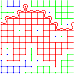
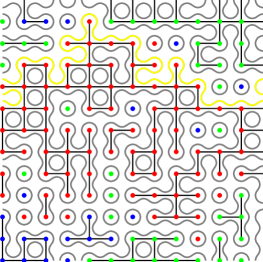
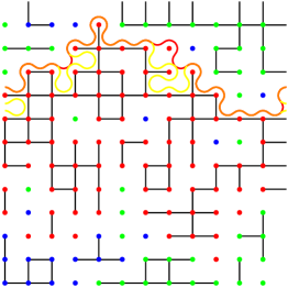
Figure 2: Various critical curves in the $3$-state Potts model. The three pictures show the same configuration with different geometrical features emphasised. (a) Spin cluster configuration. There is a non-trivial (i.e. non-homotopic to a point) red cluster wrapping along one periodic boundary condition, but not the other one. One of its boundaries is shown in red, and contributes to the fractal dimension $d_{\rm spin}=2-2h_{1,0}$. (b) Same spin configuration, but this time the FK clusters and their corresponding boundaries are shown. The non-trivial red cluster is broken into smaller FK clusters, one of them remaining non-trivial. One of the two boundaries of the percolating FK cluster is shown in yellow and has a fractal dimension $d_{\rm FK}=2-2h_{0,1}$ in the continuum limit. (c) Superposition of the previous red and yellow interfaces. Their intersection, shown in orange, corresponds to the set of points where the FK cluster touches the hull of its surrounding spin cluster. Its fractal dimension is $d_{2,1}=2-2h_{2,1}$.

5 Monte Carlo simulations

Although we the result of section 2 apply to a general excitation (5), only a few of the resulting scaling dimensions $h_{r,s}$ are relevant (i.e., $0\leq h_{r,s}<1$) for some $Q$ in the interval $0\leq Q\leq 4$. Moreover, some of the excitations are relevant only in a part of the interval, where there are not “enough colours” to realise the choice of different $\sigma_{k}$ used in (5). An example of this situation is the bulk operator $1^{1}2^{0}3^{0}$ with scaling dimension $h_{2,5}$, which is relevant only for $0\leq Q\leq 2$, meaning that $Q$ is not large enough to accommodate the three different spin colours defining the excitation.

These remarks become important if we want to measure the fractal dimension corresponding to a given excitation in a Monte Carlo simulation. For convenience we restrict the discussion to bulk critical exponents. Among the excitations which involve both spin and FK degrees of freedom, it appears that only two are relevant and physical (in the above sense). The first of these is $1^{1}$ with wrapping around the periodic direction disallowed. It describes the insertion of a spin cluster with one FK cluster inside it. The charge is $(q_{1},q_{2})=(-1,0)+(-1,-1)$ from (12)–(13) leading to the scaling dimension $h_{-2,-1}=h_{2,1}$ by application of (8). The corresponding codimension

$$d_{2,1}=2-2h_{2,1}=3-\frac{6}{\kappa}$$ (18)

is thus the fractal dimension of the set of points where the FK cluster touches the hull of its surrounding spin cluster. We have $0\leq d_{2,1}\leq 2$ for all $0\leq Q\leq 4$. An example of a geometrical curve corresponding to the dimension $d_{2,1}$ is shown in Fig. 2.

The second excitation of interest is $1^{1}2^{0}$. The charge is now $(q_{1},q_{2})=2\times(1,2)+(-1,-1)$ from (12)–(13), and the corresponding scaling dimension reads $h_{1,3}$ by (8). The fractal dimension

$$d_{1,3}=2-2h_{1,3}=4-\kappa$$ (19)

describes the same set of points as above, but with the additional constraint that a second spin cluster (the $2^{0}$ part of the label) adjacent to the one whose hull is being touched by its internal FK cluster (the $1^{1}$ part of the label) must now also propagate all the way to infinity. Note that $d_{1,3}$ and $d_{2,1}$ should coincide for the Ising model ($Q=2$) and indeed we find $d_{1,3}=d_{2,1}=1$ in this case.

We checked numerically these fractal dimensions using Monte Carlo (MC) methods. Efficient MC algorithms for the non-integer $Q$-state Potts model are already available. We chose here to work with the Chayes–Machta algorithm [15] that works for $Q\in\left[1,4\right]$. This algorithm is easy to implement and allows one to keep track of both FK and spin clusters, even for non-integer $Q$ [16].

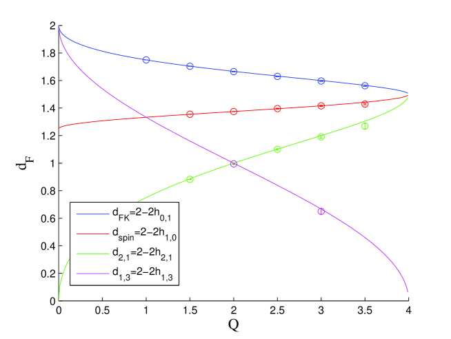
Figure 3: Fractal dimensions $d_{\rm FK}$, $d_{\rm spin}$, $d_{2,1}$ and $d_{1,3}$ (see text for details) as functions of $Q$. The small circles with their error bars are obtained from Monte Carlo simulations, while solid lines represent the CFT prediction.

The elementary step of the algorithm reads:

• Find all the FK clusters in the configuration.

• Independently label the clusters as active or inactive with respective probability $\frac{1}{Q}$ and $\frac{Q-1}{Q}$. Sites belonging to an active clusters are said to be active.

• Erase all bonds. Independently add bonds between pairs of active sites with probability $p_{c}=1-\mathrm{e}^{-K}=\frac{\sqrt{Q}}{1+\sqrt{Q}}$ . The resulting clusters are the new FK clusters.

Active sites correspond to spins in a given colour $Q_{0}$, so that the spin clusters of this colour can be obtained by performing the bond-adding step of Chayes–Machta at zero temperature, i.e. by replacing $p_{c}$ by $p_{0}=1$. The clusters and their boundaries are then detected in a standard way.

Since the fractal dimensions we wish to measure are bulk properties, we work with an $L\times L$ lattice with periodic boundary conditions. We perform the statistics on non-trivial clusters wrapping once around one of the periodic boundaries. The fractal dimensions $d_{\rm F}$ are then obtained by measuring the mean value $\ell$ of the curve length as a function of $L=32,64,\dots,800$; using the relation $\ell\sim AL^{d_{\rm F}}$.

This algorithm allowed us to recover as a check the well-known fractal dimensions of the interfaces of the FK and spin clusters, which read respectively $d_{\rm FK}=2-2h_{0,1}$ and $d_{\rm spin}=2-2h_{1,0}$. The dimension $d_{2,1}=2-2h_{2,1}$ of the set of points where the FK cluster touches the hull of its surrounding spin cluster can be measured without much more complication for $Q>1$. To evaluate the dimension $d_{1,3}=2-2h_{1,3}$, we restrict the set of points considered when measuring $d_{2,1}$ to the points whose adjacent spin cluster also wraps around the periodic boundary condition. As the Chayes–Machta for non-integer $Q$ only keeps track of one spin cluster, we were able to measure $d_{1,3}$ only for $Q$ integer. Note also that $d_{1,3}$ makes sense physically only for $Q\geq 2$.

Results are shown in Fig. 3. The agreement with our predictions is very good. The small deviations we observe when $Q$ becomes close to $Q=4$ are expected, as logarithmic corrections are known to occur in this case.

6 Conclusion

We have defined geometrical observables that keep track of both FK and spin clusters for any real $Q\in\left[0,4\right]$. We conjecture that such observables are conformally invariant and we provide exact formulas for the bulk and boundary critical exponents. Our results are supported by extensive transfer matrix and Monte Carlo computations. It is quite remarkable that all the exponents are of the Kac form $h_{r,s}$; an analytical understanding of those results would probably shed some light on this rather intriging point. We note also that we now have enough observables to cover all the Kac table $h_{r,s}$ for any integer choice of $(r,s)$, except in the two cones delimited by the straight lines $s=2r$ and $s=r/2$ (see section 2.3). This remark is particulary important in the context of Logarithmic CFT (LCFT), where including more involved geometrical observables in the theory might yield some possibly unknown, interesting logarithmic features. In particular, our transfer matrix $T$ at logarithmic points should have a much more complicated structure that the ones considered so far in lattice regularisations of LCFTs (see e.g. [7, 8]).

References

References

- [1] R.B. Potts, Math. Proc. Camb. Phil. Soc. 48, 106–109 (1952).
- [2] F.Y. Wu, Rev. Mod. Phys. 54, 235–-268 (1982).
- [3] P.P. Martin, Potts models and related problems in statistical mechanics (World Scientific, Singapore, 1991).
- [4] R.J. Baxter, Exactly solved models in statistical mechanics (Academic Press, London, 1982).
- [5] J.L. Jacobsen, Lect. Notes Phys. 775, 347–424 (2009).
- [6] M. Bauer and D. Bernard, Phys. Rep. 432, 115 (2006).
- [7] R. Vasseur, J.L. Jacobsen and H. Saleur, Nucl. Phys. B 851, 314–345 (2011).
- [8] R. Vasseur, A.M. Gainutdinov, J.L. Jacobsen and H. Saleur, arXiv:1110.1327.
- [9] C.M. Fortuin and P.W. Kasteleyn, Physica 57, 536 (1972).
- [10] H.W.J. Blöte and M.P. Nightingale, Physica A 112, 405 (1982).
- [11] J. Dubail, J.L. Jacobsen and H. Saleur, J. Phys. A: Math. Theor. 43, 482002 (2010); J. Stat. Mech. P12026 (2010).
- [12] B. Duplantier and H. Saleur, Nucl. Phys. B 290, 291 (1987).
- [13] J.L. Jacobsen and H. Saleur, Nucl. Phys. B 788, 137 (2008); J. Dubail, J.L. Jacobsen and H. Saleur, Nucl. Phys. B 813, 430 (2009); ibid. 827, 457 (2010).
- [14] H.W.J. Blöte, J.L. Cardy and M.P. Nightingale, Phys. Rev. Lett. 56, 742 (1986).
- [15] L. Chayes and J. Machta, Physica A 254, 477 (1998).
- [16] A. Zatelepin and L. Shchur, arXiv:1008.3573.