Path Integral Approach to the Calculation of Reaction Rates for a Reaction Coordinate Coupled to a Dual Harmonic Bath

Abstract

We present a new method for the numerical calculation of canonical reaction rate constants in complex molecular systems, which is based on a path integral formulation of the flux-flux correlation function. Central is the partitioning of the total system into a relevant part coupled to a dual bath. The latter consists of two parts: First, a set of strongly coupled harmonic modes, describing, for example, intramolecular degrees of freedom. They are treated on the basis of a reaction surface Hamiltonian approach. Second, a set of bath modes mimicking an unspecific environment modeled by means of a continuous spectral density. After deriving a set of general equations expressing the canonical rate constant in terms of appropriate influence functionals, several approximations are introduced to provide an efficient numerical implementation. Results for an initial application to the H-transfer in 6-Aminofulvene-1-aldimine are discussed.

INTRODUCTION

Sophisticated experimental methods nowadays provide a rather detailed insight into molecular dynamics, unraveling the importance of quantum effects even in rather complex systems at room temperature ¹. This provides a challenge to theory since a fully quantum mechanical description of condensed phase dynamics remains out of reach and therefore approximate methods have to be developed. Among the oldest problem is that of chemical reaction rates which in fact gives a straightforward means for identifying quantum tunneling in terms of the non-Arrhenius behavior. Different methods have been developed to account for quantum effects in rate calculations (see, e.g., reviews in Refs. 2, 3 which set the focus on enzyme reactions or the recent developments in Ref. 4). A rigorous formulation of quantum mechanical rate constants can be given on the basis of the path integral approach ^{5, 6, 7}, see also the related instanton type approaches, e.g. in Refs. 10, 8, 9.

Canonical rate constant are commonly calculated using the flux-flux correlation approach ⁵, which requires a path integral propagation in complex time. Here, a breakthrough in numerical efficiency has been the quasi-adiabatic propagator (QUAPI) approach developed by Makri and coworkers ^{11, 12, 13, 14}. For the case of a generic system-bath model the QUAPI approach is based on a propagator splitting where the quasi-adiabatic path along which the bath oscillators are at their minimum position along the reaction path serves as the reference. In the context of rate calculations it has been applied to the situation of a double well, bilinearly coupled to a harmonic bath ^{12, 13, 15}, and to electronically nonadiabatic reactions in Ref. 14. In another application Makri and Forsythe ¹⁶ used the all Cartesian reaction surface Hamiltonian approach ¹⁷ to determine a system-bath Hamiltonian for H diffusion in a silicon lattice. Employing a flexible bath reference for the Si environment led directly to the form of the Hamiltonian used in the QUAPI method. However, to account for the two-dimensional motion of H an effective one-dimensional Hamiltonian had been used which was supplemented by an orthogonal harmonic mode with position-dependent frequency. The Si lattice bath modes were treated at the transition state geometry, i.e. mode-mode coupling and coordinate-dependence of the Hessian were neglected. In a subsequent publication, the issue of coupled bath modes has been addressed for a generic system ¹⁸.

In the present work we consider the more general situation, where a large amplitude reaction coordinate belongs to some polyatomic molecule, which is further embedded in some environment such as a solvent or a solid state matrix. The term polyatomic molecule is assumed to include situations with strongly coupled solvation shells. This setup will be termed system coupled to a dual bath. For the case mentioned the distinction between intra- and intermolecular baths is motivated by the following observation: Quite often one faces a situation where the (intramolecular) reaction coordinate is strongly coupled to specific intramolecular modes with an interaction potential that is not of the standard bilinear form. This coupling can be well-described by a reaction surface Hamiltonian, which in principle is amenable to an ab initio treatment. For the surrounding solvent this level of sophistication is often not necessary as the spectral densities associated with the coupling are broad and featureless. This suggests a treatment in terms of empirical models or classical calculations of respective correlation functions, e.g., on the basis of molecular mechanics force fields ¹.

The goal of the present paper is to develop a path integral expression for the calculation of canonical rate constants for a reaction coordinate coupled to a dual bath. This approach is applied to the case of H-transfer in 6-Aminofulvene-1-aldimine embedded in some model environment. Although our results for this case are of preliminary character, this reaction in principle shows some interesting effects. It was investigated in detail using NMR spectroscopy by Limbach and coworkers ¹⁹. The temperature-dependent rate was found to be sensitive to the phase of the surrounding medium, which was either amorphous or crystalline. In general the reaction in the amorphous phase proceeds faster and the observed kinetic isotope effect (KIE) becomes temperature independent for low temperatures; at $T=$298 K it was $k^{\rm H}/k^{\rm D}=4$. In contrast for the crystalline environment the KIE was temperature dependent throughout the measured range, which did not include tunneling regime; at $T=$298 K it was $k^{\rm H}/k^{\rm D}=9$. The analysis of the experimental data was performed using the Bell-Limbach model ²⁰. This model introduces the reorganization energy for H-bond compression which is necessary for tunneling to occur from the intrinsic barrier for the transfer in the compressed state assuming a two step process. Further, a heavy atom mass effect is assumed for the transferred particle. Based on this model the effective barrier was estimated to be 3 kcal/mol and 1.9 kcal/mol for the crystalline and amorphous phase, respectively. In both cases the reorganization energy amounted to 0.5 kcal/mol and the mass effect was found to be 1 a.m.u. Accounting for zero-point energy effects yielded an effective barrier for D transfer of 1.2 kcal/mol and 0.7 kcal/mol for the crystalline and amorphous phase, respectively. Although this model is of empirical character it shows the importance of the specific coupling to bond-compressing intramolecular modes as well as the influence of the environment on the reaction rates, thus illustrating the essence of the present dual bath approach.

In the following we will start by introducing the system-bath Hamiltonian; a brief summary of the derivation of the intramolecular reaction surface Hamilton is given in the Appendix. Afterwards the path-integral expression of the canonical rate constant will be derived and some approximations simplifying the numerical treatment will be introduced. Subsequently, the application to the H/D-transfer in 6-Aminofulvene-1-aldimine is discussed and we conclude with a summary.

THEORY

System-Dual Bath Hamiltonian

Large amplitude motions of certain coordinates of a polyatomic molecule embedded in some environment will be described as a relevant low-dimensional system coordinate, $s$, coupled to a dual bath, where the intramolecular and environmental degrees of freedom (DOFs) are denoted $Q$ and $q$, respectively. In the Appendix we give a brief account on the derivation of a reaction surface Hamiltonian for the intramolecular problem, ²¹ specified to the case of a linear reaction path ²². The resulting intramolecular Hamiltonian can be written as the sum of the (one-dimensional) reaction coordinate part (we use mass-weighted coordinates and atomic units throughout)

$$H_{0}=-\frac{1}{2}\frac{\partial^{2}}{\partial s^{2}}+V_{0}(s)\,,$$ (1)

an intramolecular bath part

$$H_{1}=\frac{1}{2}\sum_{k}\Big{[}-\frac{\partial^{2}}{\partial Q_{k}^{2}}+\omega_{k}^{2}Q_{k}^{2}\Big{]}\,,$$ (2)

and a coupling part

$$V_{1}(s,\mbox{\boldmath$Q$})=-\sum_{k}f_{k}\left(s\right)Q_{k}+\frac{1}{2}\sum_{k,k^{\prime}}K_{kk^{\prime}}\left(s\right)Q_{k}Q_{k^{\prime}}-\frac{1}{2}\sum_{k}\omega_{k}^{2}Q_{k}^{2}$$ (3)

Here, $\mbox{\boldmath$f$}(s)$ is the vector of forces exerted on the oscillators (Eq. (A.10)), $\textbf{K}(s)$ is the reaction coordinate dependent force constant matrix, and $\omega_{k}^{2}=K_{kk}(s_{\rm ref})$ is the frequency of the $k$th bath mode at some reference value of the reaction coordinate.

The coupling of the reaction coordinate and the intramolecular DOFs to the harmonic bath of the environment,

$$H_{2}=\frac{1}{2}\sum_{\alpha}\Big{[}-\frac{\partial^{2}}{\partial q_{\alpha}^{2}}+\omega_{\alpha}^{2}q_{\alpha}^{2}\Big{]}\,,$$ (4)

will be assumed to include the lowest-order terms of a Taylor expansion with respect to $q$, i.e.

$$V_{2}(s,\mbox{\boldmath$Q$},\mbox{\boldmath$q$})=\sum_{\alpha}d_{\alpha}(s)q_{\alpha}+\sum_{\alpha,k}C_{\alpha,k}(s)Q_{k}q_{\alpha}\,.$$ (5)

Here, where $d_{\alpha}(s)$ and $c_{\alpha,k}(s)$ are some coupling functions to be specified for the system at hand. Thus the total Hamiltonian is given as

$$H=H_{0}(s)+H_{1}(\mbox{\boldmath$Q$})+H_{2}(\mbox{\boldmath$q$})+V_{1}(s,\mbox{\boldmath$Q$})+V_{2}(s,\mbox{\boldmath$Q$},\mbox{\boldmath$q$})\,.$$ (6)

Canonical Quantum Reaction Rate

We will use the flux-flux correlation function expression of the reaction rate between reactant and product, $k_{RP}$, due to Miller and coworkers ⁵

$$k_{RP}=\frac{1}{Z}\int_{0}^{\infty}C_{\rm f}(t)dt\,,$$ (7)

where

$$C_{\rm f}(t)=\mathrm{Tr}\left\{Fe^{iHt_{\rm c}^{*}}Fe^{-iHt_{\rm c}}\right\}$$ (8)

is the autocorrelation function of the symmetrized flux operator specified here to the case of a one-dimensional reaction coordinate $s$ with the dividing surface at $s=0$, $F=\frac{1}{2}\left(p_{s}\delta(s)+\delta(s)p_{s}\right)$, and $Z=\mathrm{Tr}\left(-\beta H_{\rm R}\right)$ is the canonical partition function of suitably defined reactant Hamiltonian $H_{\rm R}$. The complex time, $t_{\rm c}=t-i\beta/2$, is due to the combination of the time evolution operator and the Boltzmann operator and $\beta=1/k_{\rm B}T$.

The flux autocorrelation function can be calculated by approximating the momentum operator in the vicinity of the dividing surface by a finite difference expression with increment $\Delta s$¹²

$$C_{\rm f}(t)=\frac{1}{2\Delta s^{2}}\mathrm{Re}\left[K(\Delta s,\Delta s,0,0,t_{\rm c})-K(0,\Delta s,0,\Delta s,t_{\rm c})\right],$$ (9)

where

$$K(s,s^{\prime},s^{\prime\prime},s^{\prime\prime\prime},t_{\rm c})=\int_{-\infty}^{\infty}d\mbox{\boldmath$Q$}d\mbox{\boldmath$q$}\langle\mbox{\boldmath$Q$}|\langle\mbox{\boldmath$q$}|\langle s^{\prime\prime\prime}|e^{iHt_{\rm c}^{*}}|s^{\prime\prime}\rangle\langle s^{\prime}|e^{-iHt_{\rm c}}|s\rangle|\mbox{\boldmath$q$}\rangle|\mbox{\boldmath$Q$}\rangle\,.$$ (10)

The elementary propagators in this expression can be evaluated using the path integral technique, i.e. dividing the complex time $t_{\rm c}$ into $N$ slices. This yields ¹⁶

$$K(s_{1},s_{N+1},s_{N+2},s_{2N+2},t_{\rm c})$$ (11)

$$= \int_{-\infty}^{\infty}\cdots\int_{-\infty}^{\infty}d\mbox{\boldmath$Q$}d\mbox{\boldmath$q$}ds_{2}\cdots ds_{N}ds_{N+3}\cdots ds_{2N+1}$$

$$\times\langle\mbox{\boldmath$Q$}|\langle\mbox{\boldmath$q$}|\prod_{n=2N+1}^{N+2}\langle s_{n+1}|e^{-iH\delta_{n}}|s_{n}\rangle\prod_{n=N}^{1}\langle s_{n+1}|e^{-iH\delta_{n}}|s_{n}\rangle|\mbox{\boldmath$q$}\rangle|\mbox{\boldmath$Q$}\rangle$$

$$= \int_{-\infty}^{\infty}\cdots\int_{-\infty}^{\infty}ds_{2}\cdots ds_{N}ds_{N+3}\cdots ds_{2N+1}F_{\rm infl}(s_{1},s_{2},\cdots,s_{2N+2},t_{c})$$

$$\times\prod_{n=2N+1}^{N+2}\langle s_{n+1}|e^{-iH_{0}(s)\delta_{n}}|s_{n}\rangle\prod_{n=N}^{1}\langle s_{n+1}|e^{-iH_{0}(s)\delta_{n}}|s_{n}\rangle\,,$$

where the time steps $\delta_{n}$ are defined as follows:

$$\delta_{2N+2} = \delta_{N+2}=\frac{-t_{c}^{*}}{2N}$$

$$\delta_{n} = \frac{-t_{c}^{*}}{N},n=N+3,\cdots,2N+1$$

$$\delta_{N+1} = \delta_{1}=\frac{t_{c}}{2N}$$

$$\delta_{n} = \frac{t_{c}}{N},n=2,\cdots,N.$$ (12)

In Eq. (11) the influence functional is defined as

$$F_{\rm infl}\left(\{s_{n}\}\right)=\int_{-\infty}^{\infty}d\mbox{\boldmath$q$}d\mbox{\boldmath$Q$}\langle\mbox{\boldmath$q$}|\langle\mbox{\boldmath$Q$}|\prod_{n=2N+2}^{1}e^{-i\left[H_{1}\left(\mbox{\boldmath$Q$}\right)+V_{1}\left(s_{n},\mbox{\boldmath$Q$}\right)+H_{2}\left(\mbox{\boldmath$q$}\right)+V_{2}\left(s_{n},\mbox{\boldmath$Q$},\mbox{\boldmath$q$}\right)\right]\delta_{n}}|\mbox{\boldmath$Q$}\rangle|\mbox{\boldmath$q$}\rangle\,,$$ (13)

where $\{s_{n}\}$ denotes a specified path realization. With the help of the exact propagator for harmonic oscillators ²³ one can obtain the following result, e.g., for the intramolecular bath part

$$\langle\mbox{\boldmath$Q$}_{n+1}|e^{-i(H_{1}\left(\mbox{\boldmath$Q$}\right)+V_{1}\left(s_{n},\mbox{\boldmath$Q$}\right))\delta_{n}}|\mbox{\boldmath$Q$}_{n}\rangle=\exp\left\{-iV_{1}(s_{n},\mbox{\boldmath$Q$}_{n})\delta_{n}\right\}\prod_{k}\sqrt{\frac{\omega_{k}}{2\pi i\sin(\omega_{k}\delta_{n})}}$$

$$\times\exp\left\{\sum_{k}i\omega_{k}\left[\cot(\omega_{k}\delta_{n})Q_{nk}^{2}-\frac{Q_{n+1,k}Q_{nk}}{\sin(\omega_{k}\delta_{n})}\right]\right\}\,.$$ (14)

Note that $V_{1}(s_{n},\mbox{\boldmath$Q$}_{n})$ not only contains the force on the oscillator coordinates but also the mode-mode coupling and the change of the diagonal elements of the force constant matrix with respect to the chosen reference value of the reaction coordinate. Actually the choice of the latter does not play an important role, if one assumes that $\delta_{n}$ is chosen to be sufficiently small.

Using a similar expression for the environmental part of the Hamiltonian, we arrive at the following influence functional

$$F_{\rm infl}\left(\{s_{n}\}\right)=F_{q}F_{Q}\int_{-\infty}^{\infty}d\mbox{\boldmath$Q$}_{1}\ldots d\mbox{\boldmath$Q$}_{2N+2}d\mbox{\boldmath$q$}_{1}\ldots d\mbox{\boldmath$q$}_{2N+2}\exp\{g(\{s_{n}\},\mbox{\boldmath$Q$},\mbox{\boldmath$q$})\}$$ (15)

$$g(\{s_{n}\},\mbox{\boldmath$Q$},\mbox{\boldmath$q$}) = \sum_{nk}i\omega_{k}\left[\left(\cot(\omega_{k}\delta_{n})+\frac{(\omega_{k}\delta_{n})}{2}\right)Q_{nk}^{2}-\frac{Q_{n+1,k}Q_{nk}}{\sin(\omega_{k}\delta_{n})}\right]$$ (16)

$$+i\sum_{nk}\delta_{n}f_{k}(s_{n})Q_{nk}-\frac{i}{2}\sum_{nkk^{\prime}}Q_{nk}K_{kk^{\prime}}(s_{n})Q_{nk^{\prime}}$$

$$+\sum_{n\alpha}\frac{i\omega_{\alpha}}{\sin(\omega_{\alpha}\delta_{n})}\left[\cos(\omega_{\alpha}\delta_{n})q_{n\alpha}^{2}-q_{n+1,\alpha}q_{n\alpha}\right]$$

$$-i\sum_{n\alpha}\delta_{n}d_{\alpha}(s_{n})q_{n\alpha}-i\sum_{nk\alpha}\delta_{n}C_{\alpha k}(s_{n})Q_{nk}q_{n\alpha},$$

where

$$F_{q}=\prod_{n\alpha}\sqrt{\frac{\omega_{\alpha}}{2\pi i\sin(\omega_{\alpha}\delta_{n})}}$$ (17)

and

$$F_{Q}=\prod_{nk}\sqrt{\frac{\omega_{k}}{2\pi i\sin(\omega_{k}\delta_{n})}}$$ (18)

are path independent prefactors.

The partition function can be calculated following the same lines

$$Z = \int_{-\infty}^{\infty}\cdots\int_{-\infty}^{\infty}ds_{1}ds_{2}\cdots ds_{N_{\beta}}F_{\beta}(s_{1},s_{2},\cdots,s_{N_{\beta}})$$ (19)

$$\times \langle s_{1}|e^{-iH_{0}(s)\delta_{\beta}}|s_{N_{\beta}}\rangle\prod_{n=N_{\beta}-1}^{1}\langle s_{n+1}|e^{-iH_{0}(s)\delta_{\beta}}|s_{n}\rangle$$

with the influence functional

$$F_{\beta}\left(\{s_{n}\}\right)=\int_{-\infty}^{\infty}d\mbox{\boldmath$q$}d\mbox{\boldmath$Q$}\langle\mbox{\boldmath$q$}|\langle\mbox{\boldmath$Q$}|\prod_{n=N_{\beta}}^{1}e^{-i\left[H_{1}\left(\mbox{\boldmath$Q$}\right)+V_{1}\left(s_{n},\mbox{\boldmath$Q$}\right)+H_{2}\left(\mbox{\boldmath$q$}\right)+V_{2}\left(s_{n},\mbox{\boldmath$Q$},\mbox{\boldmath$q$}\right)\right]\delta_{\beta}}|\mbox{\boldmath$Q$}\rangle|\mbox{\boldmath$q$}\rangle\,.$$ (20)

Here $\delta_{\beta}=-{i\beta}/{N_{\beta}}$ and $N_{\beta}=2N$ is the number of time slices for the imaginary time $-i\beta$.

In a next step we need to evaluate the integrals in Eq. (15) which are of the following complex-coefficient Gaussian type

$$\int_{-\infty}^{\infty}\cdots\int_{-\infty}^{\infty}dx_{1}dx_{2}\cdots dx_{N}\exp\{-\sum_{mn}A_{mn}x_{m}x_{n}+i\sum_{mn}B_{mn}x_{m}x_{n}+\sum_{n}W_{n}x_{n}\},$$ (21)

where both $\mathbf{A}$ and $\mathbf{B}$ are real symmetric matrices. For any physically meaningful case the matrix $\mathbf{A}$ is positive-definite and the integration will converge. Moreover, it is possible to find one invertible real matrix, $\mathbf{U}_{\rm c}$, to congruently diagonalize $\mathbf{A}$ and $\mathbf{B}$ simultaneously. If $\mathbf{U_{1}}$ and $\mathbf{U_{2}}$ are orthogonal matrices such that

$$\mathbf{U_{1}}^{\rm T}\mathbf{A}\mathbf{U_{1}} = \mathbf{a}\equiv\mathrm{diag}\{a_{1},a_{2},\cdots,a_{N}\}$$

$$\mathbf{U_{2}}^{\rm T}\mathbf{a}^{-\frac{1}{2}}\mathbf{U_{1}}^{\rm T}\mathbf{B}\mathbf{U_{1}}\mathbf{a}^{-\frac{1}{2}}\mathbf{U_{2}} = \mathbf{b}\equiv\mathrm{diag}\{b_{1},b_{2},\cdots,b_{N}\}\,$$ (22)

and the matrix $\mathbf{A}$ is positive-definite such that all eigenvalues $\{a_{n}\}$ are positive, one can define the transformation matrix

$$\mathbf{U}_{\rm c}=\mathbf{U_{1}}\mathbf{a}^{-\frac{1}{2}}\mathbf{U_{2}}\,$$ (23)

which transforms $\mathbf{U}_{\rm c}^{\rm T}\mathbf{A}\mathbf{U}_{\rm c}=\mathbf{1}$ and $\mathbf{U}_{\rm c}^{\rm T}\mathbf{B}\mathbf{U}_{\rm c}=\mathbf{b}$. Using the new variables {$y_{n}$} defined by $y_{n}=\sum_{m}(\mathbf{U}_{\rm c}^{-1})_{nm}x_{m}$ the integration in Eq. (21) can be performed analytically to give

$$\int_{-\infty}^{\infty}\cdots\int_{-\infty}^{\infty}dx_{1}dx_{2}\cdots dx_{N}\exp\{-\sum_{mn}A_{mn}x_{m}x_{n}+i\sum_{mn}B_{mn}x_{m}x_{n}+\sum_{n}W_{n}x_{n}\}$$ (24)

$$= |\mathrm{Det}(\mathbf{U}_{\rm c}^{-1})|\int_{-\infty}^{\infty}\cdots\int_{-\infty}^{\infty}dy_{1}dy_{2}\cdots dy_{N}\exp\{-\sum_{n}(1-ib_{n})y_{n}^{2}+\sum_{n}w_{n}y_{n}\}$$

$$= \prod_{n}\left[\sqrt{\frac{\pi}{a_{n}}}\sqrt{\frac{1}{1-ib_{n}}}\exp\left(\frac{w_{n}^{2}}{4(1-ib_{n})}\right)\right],$$

where $w_{n}=\sum_{m}(\mathbf{U}_{\rm c})_{nm}W_{m}$. Here and in the following the square root of a complex number means its principal value, i.e., the non-negative real part.

Using this method it is at least in principle possible to solve Eq. (15). However, in practice this would imply to numerically diagonalize a large matrix for each specified path. In order to simplify matters we reconsider the environmental bath part. Here, the quadratic coefficients of the bath oscillators are path independent and assumed to be uncorrelated between each other. Based on above mentioned procedure we can find a frequency-dependent real invertible matrix $\textbf{U}_{q}(\omega)$ to congruently diagonalize each bath mode

$$\tilde{q}_{n}=\sum_{n^{\prime}}[\textbf{U}^{-1}_{q}(\omega)]_{nn^{\prime}}q_{n^{\prime}}$$ (25)

such that

$$\sum_{n}\frac{i\omega}{\sin(\omega\delta_{n})}\left[\cos(\omega\delta_{n})q_{n}^{2}-q_{n+1}q_{n}\right]=-\sum_{n}(1-ib^{q}_{n}(\omega))\tilde{q}_{n}^{2}\,,$$ (26)

where the $\{b^{q}_{n}(\omega)\}$ (and $\{a^{q}_{n}(\omega)\}$ which will appear below) are the eigenvalues from diagonalizing the corresponding coefficients matrix according the procedure introduced in Eq. (Canonical Quantum Reaction Rate). Using the new variables $\tilde{q}_{n\alpha}=\sum_{n^{\prime}}[\textbf{U}^{-1}_{q}(\omega_{\alpha})]_{nn^{\prime}}q_{n^{\prime}\alpha}$ the integration over $\{\tilde{q}_{n\alpha}\}$ can be performed analytically. The final result for influence functional is given by

$$F_{\rm infl}\left(\{s_{n}\}\right) = F_{q}F_{Q}\tilde{F_{q}}\int_{-\infty}^{\infty}\cdots\int_{-\infty}^{\infty}d\mbox{\boldmath$Q$}_{1}d\mbox{\boldmath$Q$}_{2}\cdots d\mbox{\boldmath$Q$}_{N}\exp\{g(\{s_{n}\},\mbox{\boldmath$Q$})\}$$

$$g(\{s_{n}\},\mbox{\boldmath$Q$}) = \sum_{nk}i\omega_{k}\left[\left(\cot(\omega_{k}\delta_{n})+\frac{(\omega_{k}\delta_{n})}{2}\right)Q_{nk}^{2}-\frac{Q_{n+1,k}Q_{nk}}{\sin(\omega_{k}\delta_{n})}\right]$$ (27)

$$+i\sum_{nk}\delta_{n}f_{k}(s_{n})Q_{nk}-\frac{i}{2}\sum_{nkk^{\prime}}Q_{nk}K_{kk^{\prime}}(s_{n})Q_{nk^{\prime}}+\Delta(\{s_{n}\})$$

$$+i\sum_{nk}\delta_{n}\Delta f_{k}(s_{n})Q_{nk}+\sum_{nkn^{\prime}k^{\prime}}g_{nk,n^{\prime}k^{\prime}}(s_{n},s_{n^{\prime}})Q_{nk}Q_{n^{\prime}k^{\prime}},$$

where

$$\tilde{F_{q}}=\prod_{n\alpha}\sqrt{\frac{\pi}{a^{q}_{n}(\omega_{\alpha})}}\sqrt{\frac{1}{(1-ib^{q}_{n}(\omega_{\alpha}))}}$$ (28)

$$\Delta(\{s_{n}\}) = \sum_{n\alpha}\frac{w_{n\alpha}^{2}}{4[1-ib^{q}_{n}(\omega_{\alpha})]}$$

$$w_{n\alpha} = -i\sum_{n^{\prime}}[\textbf{U}_{q}(\omega_{\alpha})]_{n^{\prime}n}\delta_{n^{\prime}}d_{\alpha}(s_{n^{\prime}})$$

$$\Delta f_{k}(s_{n}) = \sum_{n^{\prime}\alpha}\frac{w_{n^{\prime}\alpha}u_{n^{\prime}\alpha,nk}}{2[1-ib^{q}_{n^{\prime}}(\omega_{\alpha})]}$$

$$u_{n^{\prime}\alpha,nk}(s_{n}) = -i[\textbf{U}_{q}(\omega_{\alpha})]_{nn^{\prime}}\delta_{n}C_{\alpha k}(s_{n})$$

$$g_{nk,n^{\prime}k^{\prime}}(s_{n},s_{n^{\prime}}) = \sum_{n^{\prime\prime}\alpha}\frac{u_{n^{\prime\prime}\alpha,nk}u_{n^{\prime\prime}\alpha,n^{\prime}k^{\prime}}}{4[1-ib^{q}_{n^{\prime\prime}}(\omega_{\alpha})]}.$$ (29)

So far the $q$-integrations have been performed following the idea from Eq. (21) to Eq. (24). The quantities entering Eq. (Canonical Quantum Reaction Rate) can be calculated readily before the $Q$-integrations. In a final step the procedure of Eq. (Canonical Quantum Reaction Rate) can be applied to the $Q$-integrations to numerically diagonalize the complex coefficient matrix in Eq. (Canonical Quantum Reaction Rate) for each path of the reaction coordinate. The final result for the influence functional of the reaction coordinate plus dual bath system can then be formally written as:

$$F_{\rm infl}\left(\{s_{n}\}\right)=F_{q}F_{Q}\tilde{F_{q}}e^{\Delta(\{s_{n}\})}\prod_{nk}\left(\sqrt{\frac{\pi}{a^{Q}_{nk}}}\sqrt{\frac{1}{1-ib^{Q}_{nk}}}\exp\Big{\{}\frac{w_{nk}^{2}}{4(1-ib^{Q}_{nk})}\Big{\}}\right)\,.$$ (30)

with the different functions defined in Eqs.(17), (18) and (28). The quantities $a_{nk}^{Q}$, $b_{nk}^{Q}$, and $w_{nk}$ in above formal expression can be obtained from the numerical diagonalization of the respective complex coefficient matrix.

Approximations

Depending on the system size obtaining the quantities in Eq. (30) by direct diagonalization might become rather time consuming, due to those terms which depend on the system’s coordinate and, therefore, have to be evaluated for each specific path. Therefore, we will introduce certain approximations to make the approach numerical efficient for such cases.

First, we will assume that the coupling strength between the $Q_{k}$ and $q_{\alpha}$ modes does not strongly depend on $s$. Thus we ignore the $s$-dependence of the coupling strength between $Q_{k}$ and $q_{\alpha}$, i.e, $\{C_{\alpha k}\}$ are simply constants and hence $\{g_{nk,n^{\prime}k^{\prime}}(s_{n},s_{n^{\prime}})=g_{nk,n^{\prime}k^{\prime}}\}$ are also constants. Next, we assume that not for all modes, $\{Q_{k}\}$, the mode mixing due to $\mathbf{K}(s)$ shows a strong coordinate dependence. In the following we use $\{Q_{k}\}$ to denote those intramolecular DOFs, which are most strongly affected by the motion of the reaction coordinate $s$. The remaining intramolecular modes are comprised in $\{Q_{\nu}\}$. For the latter modes, the quadratic coefficients will be replaced by their $s$-independent mean values along the reaction path in Eq. (Canonical Quantum Reaction Rate), i.e.,

$$K_{\nu\nu^{\prime}}(s_{n})\rightarrow\langle K_{\nu\nu^{\prime}}\rangle\equiv\frac{1}{2L}\int_{-L}^{L}K_{\nu\nu^{\prime}}(s)ds,$$ (31)

where $2L$ is the length of the reaction path. Under this approximation, we need to diagonalize a large matrix just once, while for each specified path we only need to diagonalize a much smaller matrix since only a few DOFs, $\{Q_{k}\}$, are significantly coupled via $s$.

Following the idea of Eq. (Canonical Quantum Reaction Rate) we can find a real invertible matrix $\mathbf{U^{Q}}$ which congruently diagonalizes the quadratic coefficient matrix related only to $\{Q_{\nu}\}$

$$\sum_{n\nu}i\omega_{\nu}\left[\left(\cot(\omega_{\nu}\delta_{n})+\frac{(\omega_{\nu}\delta_{n})}{2}\right)Q_{n\nu}^{2}-\frac{Q_{n+1,\nu}Q_{n\nu}}{\sin(\omega_{\nu}\delta_{n})}\right]$$ (32)

$$-\frac{i}{2}\sum_{n\nu\nu^{\prime}}\delta_{n}\langle K_{\nu\nu^{\prime}}\rangle Q_{n\nu}Q_{n\nu^{\prime}}+\sum_{n\nu,n^{\prime}\nu^{\prime}}g_{n\nu,n^{\prime}\nu^{\prime}}Q_{n\nu}Q_{n^{\prime}\nu^{\prime}}$$

$$= -\sum_{n\nu}(1-ib_{n\nu})\tilde{Q}_{n\nu}^{2},$$

where $\tilde{Q}_{n\nu}=\sum_{n^{\prime}\nu^{\prime}}\left(\mathbf{U^{Q}}\right)^{-1}_{n\nu,n^{\prime}\nu^{\prime}}Q_{n\nu^{\prime}}$. With the help of this transformation we can analytically integrate over the $\{\tilde{Q}_{n\nu}\}$ part. This will further contribute a pre-factor $\tilde{F_{Q}}$ and some modifications to the exponential factor compared with Eq. (Canonical Quantum Reaction Rate)

$$F_{\rm infl}\left(\{s_{n}\}\right) = F_{q}F_{Q}\tilde{F_{q}}\tilde{F_{Q}}\int_{-\infty}^{\infty}\cdots\int_{-\infty}^{\infty}d\mbox{\boldmath$Q$}_{1}d\mbox{\boldmath$Q$}_{2}\cdots d\mbox{\boldmath$Q$}_{N}\exp\{g(\{s_{n},Q_{nk}\})\}$$

$$g(\{s_{n},Q_{nk}\}) = \sum_{nk}i\omega_{k}\left[\left(\cot(\omega_{k}\delta_{n})+\frac{(\omega_{k}\delta_{n})}{2}\right)Q_{nk}^{2}-\frac{Q_{n+1,k}Q_{nk}}{\sin(\omega_{k}\delta_{n})}\right]$$ (33)

$$+i\sum_{nk}\delta_{n}f_{k}(s_{n})Q_{nk}-\frac{i}{2}\sum_{nkk^{\prime}}Q_{nk}K_{kk^{\prime}}(s_{n})Q_{nk^{\prime}}+\Delta(\{s_{n}\})$$

$$+i\sum_{nk}\delta_{n}\Delta f_{k}(s_{n})Q_{nk}+\sum_{nkn^{\prime}k^{\prime}}g_{nk,n^{\prime}k^{\prime}}Q_{nk}Q_{n^{\prime}k^{\prime}}+\tilde{\Delta}(\{s_{n}\})$$

$$+i\sum_{nk}\delta_{n}\Delta\tilde{f}_{k}(s_{n})Q_{nk}+\sum_{nkn^{\prime}k^{\prime}}\tilde{g}_{nk,n^{\prime}k^{\prime}}Q_{nk}Q_{n^{\prime}k^{\prime}},$$

where

$$\tilde{F}_{Q}=\prod_{n\nu}\sqrt{\frac{\pi}{a_{n\nu}}}\sqrt{\frac{1}{1-ib_{n\nu}}}$$ (34)

and the additional terms caused by the reduction of DOFs are defined as follows:

$$\tilde{\Delta}(\{s_{n}\}) = \sum_{n\nu}\frac{w_{n\nu}^{2}}{4(1-ib_{n\nu})}$$

$$w_{n\nu} = \sum_{n^{\prime}\nu^{\prime}}(\mathbf{U^{Q}})_{n^{\prime}\nu^{\prime},n\nu}\left[i\delta_{n^{\prime}}f_{\nu^{\prime}}(s_{n^{\prime}})+i\delta_{n^{\prime}}\Delta f_{\nu^{\prime}}(s_{n^{\prime}})\right]$$

$$\Delta\tilde{f}_{k}(s_{n}) = \sum_{n^{\prime}\nu^{\prime}}\frac{w_{n^{\prime}\nu^{\prime}}u_{nk,n^{\prime}\nu^{\prime}}}{2(1-ib_{n^{\prime}\nu^{\prime}})}$$

$$u_{nk,n^{\prime}\nu^{\prime}} = 2\sum_{n^{\prime\prime}\nu}(\mathbf{U^{Q}})_{n^{\prime\prime}\nu,n^{\prime}\nu^{\prime}}g_{nk,n^{\prime\prime}\nu}-i\sum_{\nu}(\mathbf{U^{Q}})_{n\nu,n^{\prime}\nu^{\prime}}\delta_{n}K_{k\nu}(s_{n})$$

$$\tilde{g}_{nk,n^{\prime}k^{\prime}}(s_{n},s_{n^{\prime}}) = \sum_{n^{\prime\prime}\nu}\frac{u_{nk,n^{\prime\prime}\nu}u_{n^{\prime}k^{\prime},n^{\prime\prime}\nu}}{4(1-ib_{n^{\prime\prime}\nu})}\,.$$ (35)

Similar to Eq. (30) the final result can be written formally as

$$F_{\rm infl}\left(\{s_{n}\}\right)=F_{q}F_{Q}\tilde{F}_{q}\tilde{F}_{Q}e^{\Delta(\{s_{n}\})+\tilde{\Delta}(\{s_{n}\})}\prod_{nk}\left(\sqrt{\frac{\pi}{a^{Q}_{nk}}}\sqrt{\frac{1}{1-ib^{Q}_{nk}}}\exp\Big{\{}\frac{w_{nk}^{2}}{4(1-ib^{Q}_{nk})}\Big{\}}\right).$$

with the different functions defined in Eqs.(17), (18), (28), and (34). The quantities $a_{nk}^{Q}$, $b_{nk}^{Q}$, and $w_{nk}$ in above formal expression can be obtained from the numerical diagonalization of the complex coefficient matrix and the final sum is only for modes which strongly couple to $s$. The final numerical calculations may start from Eq. (Approximations) which is feasible since only a very low-dimensional matrix (according to the coordinates $\{Q_{k}\}$) needs to be diagonalized for each specified path.

APPLICATION TO THE H/D-TRANSFER IN 6-AMINOFULVENE-1-ALDIMINE

In this section we present results of a preliminary simulation based on a reaction surface model Hamiltonian describing the intramolecular H atom transfer in 6-Aminofulvene-1-aldimine. Here, our aim is not to provide a quantitative assessment of this reaction, but to illustrate the theoretical formalism presented in the previous section. The configuration of two stationary points, which have been obtained at the B3LYP/6-31+G(d,p) level of theory²⁴ are shown in Fig. 1 . The minimum configuration in panel (a) corresponds to the reactant or equivalent product. The H atom transfer process can take place from the reactant via the transition state (panel (b)) to the product or inversely. The reaction barrier height, as calculated by the energy difference of the minimum and the transition state, is 3.8 kcal/mol (fully relaxed gas phase barrier).

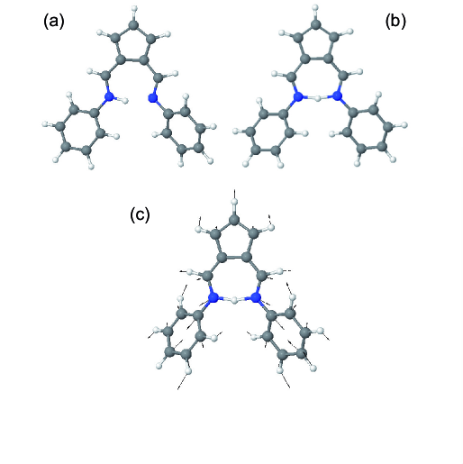
Figure 1: 6-Aminofulvene-1-aldimine: (a) minimum configuration, (b) transition state for the hydrogen atom transfer, (c) Strongly coupled normal mode at the transition state having a frequency of 641 cm^-1. All results have been obtained at the B3LYP/6-31+G(d,p) level of theory.

The unit vector which defines the linear reaction path is given by the direction pointing from the equivalent reactant to the product, i.e., $\mbox{\boldmath$e$}_{s}=(\mbox{\boldmath$R$}_{\rm prod}-\mbox{\boldmath$R$}_{\rm reac})/(|\mbox{\boldmath$R$}_{\rm prod}-\mbox{\boldmath$R$}_{\rm reac}|)$ (cf. Fig. 1). The potential along the one-dimensional linear reaction path coordinate, $V(\mbox{\boldmath$R$}_{0})$, is shown in Fig. 2. According to the present linear reaction path, the barrier is as high as 14.85 kcal/mol.

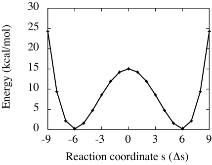
Figure 2: The zeroth-order potential energy curve, $V(\mbox{\boldmath$R$}_{0})$, obtained at the B3LYP/6-31+G(d,p) level of theory for the hydrogen/deuterium atom transfer reaction in 6-Aminofulvene-1-aldimine as shown in Fig. 1. The curve has been generated from 19 points, symmetrically distributed with respect to the reference geometry $s_{\rm ref}=0$, which corresponds to $\mbox{\boldmath$R$}_{\rm ref}=(\mbox{\boldmath$R$}_{\rm prod}-\mbox{\boldmath$R$}_{\rm reac})/2$. The reactant/product configuration is at $s=\pm 6\Delta s$, i.e. $\Delta s=|\mbox{\boldmath$R$}_{\rm prod}-\mbox{\boldmath$R$}_{\rm reac}|/12$.

Within the harmonic approximation for the intramolecular bath modes, the energy difference with respect to the fully relaxed reaction path will be recovered by the so-called bath reorganization energy ²¹ (see also discussion in Refs. 25 and 26 where two and three reaction coordinates, respectively, have been used to obtain a better agreement with the fully relaxed barrier even without taking into account coupled harmonic vibrations). Furthermore, in the real system, there will be a contribution to the reorganization energy due to the interaction with the environment. In the following we do not attempt to fit the environmental contribution such as to obtain agreement with the experimental estimate by Limbach and coworkers. ¹⁹

The considered molecule has 105 intramolecular vibrational degrees of freedom, whose couplings to the reaction coordinate, i.e. $f_{k}(s)$, and $K_{k,k^{\prime}}(s)$, can be obtained as described in the Appendix, Eq. (Linear Reaction Surface Hamiltonian). For the reference $\mbox{\boldmath$R$}_{\rm ref}$ we have chosen the point midway between reactant and product along the one-dimensional reaction path. For the present illustration we have selected only one strongly coupled mode $Q_{k}$ for explicit consideration. The displacement vectors are shown in Fig. 2c. Apparently this mode symmetrically modifies the H-bond length and therefore modulates the reaction barrier. The remaining intramolecular modes as well as possible environmental modes are comprised into the bath $q$. In other words, we have simplified matters and started directly from Eq. (Canonical Quantum Reaction Rate).

The coupling between the environment $q$ and the intra-molecular DOFs, $s$ and $Q_{k}$, are defined as

$$d_{\alpha}(s) = d_{1}e^{-\omega_{\alpha}^{2}/d_{2}^{2}}(s+\eta s^{2})$$

$$C_{\alpha,k}(s) = C_{\alpha,k}=c_{1}e^{-(\omega_{k}-\omega_{\alpha})^{2}/c_{2}^{2}},$$ (36)

where $d_{1}$, $d_{2}$, $\omega_{0}$, $\eta$, $c_{1}$, and $c_{2}$ are parameters. The $s$-dependence of $d_{\alpha}(s)$ has been expanded to second-order and the bath frequency dependence has been simply chosen to be of Gaussian form. The environmental modes are assumed to have uniform density of states in the region, where we take into account the coupling with the molecular DOFs.

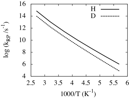
Figure 3: The calculated temperature dependence of H/D transfer rate constants, Eq. (7), in the thermal activation region based on a one-dimensional linear reaction path, $s$, coupled to one intra-molecular mode, $Q_{k}$, and 50 bath modes, $q$. In the simulation the reaction coordinate integration has been replaced by a sum over the three points, $s=-1,0,1$. For the partition function of the reactant these points were chosen as $s=-7,-6,-5$. The number of time slices has been $N=4$.

The calculated canonical rates, Eq. (7), obtained from this preliminary model Hamiltonian are shown in Fig. 3. At 298 K the KIE is $k_{RP}^{H}/k_{RP}^{D}=10$, when the following coupling parameters are used: $c_{1}=d_{1}=$(0.628 kcal/mol)², $c_{2}=d_{2}=6.28$ kcal/mol, and $\eta=0.2\Delta s^{-1}$. The involved bath frequency region covers the range from 3 to 30 kcal/mol with 50 harmonic oscillators equally distributed. Given the fact that the experimental KIE ranges between 4 and 9 and strongly depends on the phase of the environment, the present order-of-magnitude agreement is rather reasonable given the simple model for the system-bath coupling. Further, we note that the same holds true for the absolute values of the rates. However, the obtained values for the activation energies (slopes of curves in Fig. 3) deviate from the experimental ones. In Ref. 19 it was found that the rate between the thermal activation energies between the H and the D case is about 2/3. In the present simulation the activation energies are about 3-4 times the experimental ones and the difference between the activation energies of different isotopomers are too small. The latter fact is not surprising since the shapes of potential curves for hydrogen and deuterium transfers are the same and the only difference lies in the length of the step $\Delta s$ which appears in Eq. (9). The ratio for the steps is only slightly different from one, $\Delta s(H)/\Delta s(D)=0.9978$. In order to improve the description at this point, more intramolecular vibrational modes need to be taken into account. This would lower the effective reaction barrier due to reorganization energy contributions and therefore the activation energy. On the other hand, due to the isotope dependent effective coupling, the difference between H and D activation energies would become more pronounced.

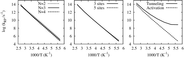
Figure 4: The left and middle panels show the convergence of the thermal activation energy (the slope) for H-transfer in the high temperature region by only considering configurations which are important for thermal activation, i.e., around $s=0$. In the left panel the dependence on the number of time slices $N$ is shown for $s=-1,0,1$ and in the middle panel the case $s=-2,-1,0,1,2$ is given for $N=4$.The right panel shows the quantum tunneling effects in the low-temperature region by covering some configurations which are important for tunneling ($s=-2,-1,0,1,2$ (dashed curve) and $s=-5,-1,0,1,5$ (solid curve)).

The numerical effort in the calculation of the propagator in Eq. (11) by path integration depends on the number of time slices, $N$, as well as on the method for evaluating the multi-dimensional integrals of the reaction path coordinates, $s_{n}$. For the present application in Fig. 3 the focus has been on the thermal activation range, i.e. the high-temperature regime. This allowed us to simplify the rate calculation by performing the integration as a sum over three points in the vicinity of the reaction barrier, $s=-1,0,1$. In Fig. 4 (middle panel) we show the dependence on the number of discretization points for $N=4$ time slices. Specifically, we have chosen $s=-2,-1,0,1,2$. The ignorable difference shows the applicability of the simplification technique, which we have adopted for the high temperature calculations. The dependence on the number of time-slices is shown in the left panel of Fig. 4. Clearly, the variation for the covered range, $N=2,3,4$, is rather small, justifying our choice of $N=4$ in Fig. 3. Finally, we address the issue of tunneling in the right panel of Fig. 4. In principle, accounting for quantum tunneling at low temperatures requires to include configurations, which are located near the turning point corresponding to the energy of the tunneling particle. In order to illustrate this point, we present results for five discretization points, i.e. $s=-2,-1,0,1,2$ (dashed curve) and $s=-5,-1,0,1,5$ (solid curve). The change of the mechanism from thermal activation to tunneling is apparent from the quite different temperature dependence of the rates. In passing we note that a systematic study of different discretizations might give an indication for those configurations that contribute to the tunneling process.

SUMMARY

We have developed a path integral method for the determination of canonical reaction rates for the case of a reaction coordinate coupled to a dual bath. The latter is comprised of an intramolecular part, which is modeled using the reaction surface Hamiltonian approach, and an intermolecular (solvent) part. Such a partition of the interactions into different structurally motivated levels appears to be most suitable for the description of intramolecular proton or H-atom transfer reactions. The formulation benefits from the harmonic oscillator nature of the intra- and intermolecular baths in two respects: First, it enables us to perform the integration over the bath variables and second the reaction surface Hamiltonian method provides a means to determine intramolecular Hamiltonian parameters from first principles. This involves couplings between normal modes along the reaction path due to the non-diagonal Hessian matrix, which require a diagonalization for each specified path and thus substantial numerical effort. We have suggested an approximation which amounts to the replacement of the reaction coordinate dependent Hessian by its averaged value for less strongly coupled intramolecular modes.

The initial application has been to the H/D transfer in 6-Aminofulvene-1-aldimine. Despite the various additional approximations in this application it could be shown, that our approach can give reasonable (i.e. order-of-magnitude) estimates for the reaction rates. Further work on this particular reaction shall be directed to obtain an improved description of the reaction surface as well as a realistic model for the interaction with the environment.

ACKNOWLEDGMENTS

We gratefully acknowledge financial support by the Deutsche Forschungsgemeinschaft through the GK 788 at the Freie Universität Berlin. Y. Yang also acknowledges financial support from National Natural Science Foundation of China under Grant No. 11004125.

APPENDIX

Reaction Surface Hamiltonian

The reaction surface Hamiltonian combines the description of several large amplitude coordinates {$s_{\alpha}$} coupled to many small amplitude displacements {$Q_{k}$}. ^{27, 28, 25} To generate this Hamiltonian from the exact Cartesian coordinate Hamiltonian we can directly exploit our recently developed kinetic energy quantization method. ²⁹

Suppose that we have the Cartesian Hamiltonian

$$H\left(\mbox{\boldmath$R$}\right) = T\left(\mbox{\boldmath$R$}\right)+V\left(\mbox{\boldmath$R$}\right)$$

$$T\left(\mbox{\boldmath$R$}\right) = \frac{1}{2}\mbox{\boldmath$P$}^{2}=-\frac{1}{2}\frac{\partial^{2}}{\partial\mbox{\boldmath$R$}^{2}}\,,$$ (A.1)

where $R$ is the $3N$-dimensional vector of mass-weighted Cartesian coordinates for system with $N$ atoms and $\mbox{\boldmath$P$}=-i\partial/\partial\mbox{\boldmath$R$}$ is the corresponding linear momentum operator. Suppose that there is a reaction surface defined by a function along the reaction coordinates $s$, i.e.,

$$\mbox{\boldmath$R$}=\mbox{{\boldmath$R$}${}_{0}$}\left(\mbox{\boldmath$s$}\right)\,.$$ (A.2)

The potential energy function, $V\left(\mbox{\boldmath$R$}\right)$, is expanded around the reaction surface as follows

$$V\left(\mbox{\boldmath$R$}\right)\approx V\left(\mbox{{\boldmath$R$}${}_{0}$}\left(\mbox{\boldmath$s$}\right)\right)+\Delta\mbox{\boldmath$R$}(\mbox{\boldmath$s$})^{\rm T}\frac{\partial V}{\partial\mbox{\boldmath$R$}}\Big{|}_{{}_{\mbox{{\boldmath$R$}${}_{0}$}\left(\mbox{\boldmath$s$}\right)}}+\frac{1}{2}\Delta\mbox{\boldmath$R$}(\mbox{\boldmath$s$})^{\rm T}\frac{\partial^{2}V}{\partial\mbox{\boldmath$R$}^{2}}\Big{|}_{{}_{\mbox{{\boldmath$R$}${}_{0}$}\left(\mbox{\boldmath$s$}\right)}}\Delta\mbox{\boldmath$R$}(\mbox{\boldmath$s$})\,,$$ (A.3)

where $\Delta\mbox{\boldmath$R$}\left(\mbox{\boldmath$s$}\right)=\mbox{\boldmath$R$}-\mbox{{\boldmath$R$}${}_{0}$}\left(\mbox{\boldmath$s$}\right)$. The reaction surface is defined in such a way that the potential energy $V\left(\mbox{\boldmath$R$}\right)$ can be approximated by low-order orthogonal displacements, i.e., Eq. (A.3) can be truncated in the given form.

To obtain the reaction surface Hamiltonian we first need to define the new coordinates, i.e., the reaction coordinates {$s_{\alpha}$} and the orthogonal displacements {$Q_{k}$}. The former are already defined by the reaction surface as well as the unit vectors {$\mbox{\boldmath$e$}_{\alpha}\left(\mbox{\boldmath$s$}\right)$} according to which we have the reaction coordinate vector

$$\mbox{\boldmath$s$}=\sum_{\alpha=1}^{D}s_{\alpha}\mbox{\boldmath$e$}_{\alpha}\left(\mbox{\boldmath$s$}\right).$$ (A.4)

To get the latter we need a projection operator to project out the reaction coordinate $s$

$$\mathcal{P\left(\mbox{\boldmath$s$}\right)}=1-\sum_{\alpha}\mbox{\boldmath$e$}_{\alpha}\mbox{\boldmath$e$}_{\alpha}^{\rm T}.$$ (A.5)

Then we can diagonalize the projected Hessian matrix $\mathbf{K}\left(\mbox{\boldmath$s$}\right)$ for each point of the reaction surface by an orthogonal transformation $\mathbf{U}_{\rm RS}\left(\mbox{\boldmath$s$}\right)$

$$\mathbf{U}_{RS}\left(\mbox{\boldmath$s$}\right)^{\dagger}\mathbf{K}\left(\mbox{\boldmath$s$}\right)\mathbf{U}_{\rm RS}\left(\mbox{\boldmath$s$}\right)={\rm diag}\{\cdots\omega_{\alpha}^{2}\left(\mbox{\boldmath$s$}\right)\cdots\omega_{g}^{2}\left(\mbox{\boldmath$s$}\right)\cdots\omega_{k}^{2}\left(\mbox{\boldmath$s$}\right)\cdots\},$$ (A.6)

where $\mathbf{K}\left(\mbox{\boldmath$s$}\right)=\mathcal{P\left(\mbox{\boldmath$s$}\right)}\partial^{2}V/\partial\mbox{\boldmath$R$}^{2}|_{\mbox{{\boldmath$R$}${}_{0}$}}\mathcal{P\left(\mbox{\boldmath$s$}\right)}$ is a real symmetric matrix.

In total there are $D+6$ zero eigenvalues $\{\omega_{\alpha}^{2}\}$ and $\{\omega_{g}^{2}\}$ corresponding to the reaction coordinates and six-dimensional global translation and rotation, respectively. The orthogonal transformation matrix contains the corresponding eigenvectors of $\mathbf{K}\left(\mbox{\boldmath$s$}\right)$

$$\mathbf{U}_{\rm RS}\left(\mbox{\boldmath$s$}\right)=\left(\cdots\mbox{\boldmath$e$}_{\alpha}\left(\mbox{\boldmath$s$}\right)\cdots\mbox{\boldmath$e$}_{g}\left(\mbox{\boldmath$s$}\right)\cdots\mbox{\boldmath$e$}_{k}\left(\mbox{\boldmath$s$}\right)\cdots\right).$$ (A.7)

The six-dimensional global translation and rotation as well as the $3N-6-D$ displacements orthogonal to the reaction surface are defined by

$$R_{g} = \mbox{\boldmath$e$}_{g}^{\rm T}\Delta\mbox{\boldmath$R$}$$

$$Q_{k} = \mbox{\boldmath$e$}_{k}^{\rm T}\Delta\mbox{\boldmath$R$}.$$ (A.8)

The original $3N$-dimensional vector is now expressed with the new unit vectors

$$\mbox{\boldmath$R$}=\mbox{\boldmath$R$}_{\rm ref}+\sum_{\alpha}s_{\alpha}\mbox{\boldmath$e$}_{\alpha}+\sum_{g}R_{g}\mbox{\boldmath$e$}_{g}+\sum_{k}Q_{k}\mbox{\boldmath$e$}_{k},$$ (A.9)

where the reference geometry $\mbox{\boldmath$R$}_{\rm ref}=\mbox{{\boldmath$R$}${}_{0}$}\left(\mbox{\boldmath$s$}=0\right)$ is the origin of the new coordinates system.

Based on the knowledge of the new coordinates it is not difficult to find the potential energy

$$V\left(\mbox{\boldmath$s$},\mbox{\boldmath$Q$}\right)=V(\mbox{{\boldmath$R$}${}_{0}$}\left(\mbox{\boldmath$s$}\right))-\sum_{k}f_{k}\left(\mbox{\boldmath$s$}\right)Q_{k}+\frac{1}{2}\sum_{k}\omega_{k}\left(\mbox{\boldmath$s$}\right)^{2}Q_{k}^{2},$$ (A.10)

where $f_{k}\left(\mbox{\boldmath$s$}\right)=-\mbox{\boldmath$e$}_{k}^{\rm T}\partial V/\partial\mbox{\boldmath$R$}|_{\mbox{{\boldmath$R$}${}_{0}$}}$. It is obvious that the potential energy does not depend on $\{\mbox{\boldmath$R_{g}$}\}$, however, the kinetic energy operator (KEO) does depend on $\{\mbox{\boldmath$R_{g}$}\}$ and normally it is not possible to separate them exactly. According to Ref. 29 the following formal KEO can be obtained

$$T=\frac{1}{2}\tilde{\mbox{\boldmath$P$}}^{{\dagger}}\frac{\partial\tilde{\mbox{\boldmath$R$}}}{\partial\mbox{\boldmath$R$}}\left(\frac{\partial\tilde{\mbox{\boldmath$R$}}}{\partial\mbox{\boldmath$R$}}\right)^{\rm T}\tilde{\mbox{\boldmath$P$}},$$ (A.11)

where $\tilde{\mbox{\boldmath$R$}}^{\rm T}=\left(\begin{array}[]{ccc}\mbox{\boldmath$s$}^{\rm T}&\mbox{\boldmath$R_{g}$}^{\rm T}&\mbox{\boldmath$Q$}^{\rm T}\\ \end{array}\right)$ is the full set of the new coordinates and $\tilde{\mbox{\boldmath$P$}}=-i\partial/\partial\tilde{\mbox{\boldmath$R$}}$. According to Ref. 29 all components of $\tilde{\mbox{\boldmath$P$}}$ are Hermitian due to the orthogonality of transformation except $\mbox{\boldmath$P$}_{\mbox{\boldmath$s$}}$. Eq. (A.11) has a fully coupled form in case of a general reaction surface. The factor which is responsible for complexity when it comes to a numerical implementation is that all unit vectors depend on $s$, i.e., the orthogonal transformation matrix $\mathbf{U}_{\rm RS}\left(\mbox{\boldmath$s$}\right)$ depends on $s$ thus we have to calculate the derivatives with respect to $s$.

Linear Reaction Surface Hamiltonian

In the following we will simplify the KEO, Eq. (A.11), by choosing a different representation in terms of constant unit vectors that describe the reaction coordinates $s$ for the special case of a linear reaction surface. ²² With the help of certain predefined constant unit vectors $\{\mbox{\boldmath$e$}_{\alpha}\}$ we can obtain the following equation for the linear reaction surface

$$\mbox{{\boldmath$R$}${}_{0}$}\left(\mbox{\boldmath$s$}\right)=\mbox{\boldmath$R$}_{\rm ref}+\sum_{\alpha}s_{\alpha}\mbox{\boldmath$e$}_{\alpha}.$$ (A.12)

The coordinate transformations are modified as follows:

$$R = \mbox{{\boldmath$R$}${}_{0}$}\left(\mbox{\boldmath$s$}\right)+\sum_{k}Q_{k}\mbox{\boldmath$e$}_{k}=\mbox{\boldmath$R$}_{\rm ref}+\sum_{\alpha}s_{\alpha}\mbox{\boldmath$e$}_{\alpha}+\sum_{k}Q_{k}\mbox{\boldmath$e$}_{k}$$

$$s_{\alpha} = \mbox{\boldmath$e$}_{\alpha}^{\rm T}\Delta\mbox{\boldmath$R$},\hskip 28.45274ptQ_{k}=\mbox{\boldmath$e$}_{k}^{\rm T}\Delta\mbox{\boldmath$R$},$$ (A.13)

where $\Delta\mbox{\boldmath$R$}=\mbox{\boldmath$R$}-\mbox{\boldmath$R$}_{\rm ref}$ is different from $\Delta\mbox{\boldmath$R$}\left(\mbox{\boldmath$s$}\right)$ in Eq. (A.3) while $\{Q_{k}\}$ and $\{\mbox{\boldmath$e$}_{k}\left(\mbox{\boldmath$s$}\right)\}$ have the same definition as in the previous section. Note that we have combined the $\{R_{g}\}$ and $\{Q_{k}\}$ into the same set of indexes $\{Q_{k}\}$ to simplify the notation. With the help of Eq. (A.11) and Eq. (Linear Reaction Surface Hamiltonian) we can derive a simplified KEO for a linear reaction surface. First, we calculate the elements of the Jacobi matrices starting from Eq. (Linear Reaction Surface Hamiltonian). Using the chain rule to calculate the derivatives from Eq. (Linear Reaction Surface Hamiltonian) leads to the following results

$$\frac{\partial s_{\alpha}}{\partial\mbox{\boldmath$R$}} = \mbox{\boldmath$e$}_{\alpha}^{\rm T}$$

$$\frac{\partial Q_{k}}{\partial\mbox{\boldmath$R$}} = \mbox{\boldmath$e$}_{k}^{\rm T}+\sum_{\alpha}\mbox{\boldmath$e$}_{\alpha}^{\rm T}\left(\Delta\mbox{\boldmath$R$}^{\rm T}\frac{\partial\mbox{\boldmath$e$}_{k}}{\partial s_{\alpha}}\right)\,.$$ (A.14)

Thus the elements for the matrix products in Eq. (A.11) can be obtained as follows

$$\left(\frac{\partial\mbox{\boldmath$s$}}{\partial\mbox{\boldmath$R$}}\left(\frac{\partial\mbox{\boldmath$s$}}{\partial\mbox{\boldmath$R$}}\right)^{\rm T}\right)_{\alpha\beta} = \mbox{\boldmath$e$}_{\alpha}^{\rm T}\mbox{\boldmath$e$}_{\beta}=\delta_{\alpha\beta}$$

$$\left(\frac{\partial\mbox{\boldmath$s$}}{\partial\mbox{\boldmath$R$}}\left(\frac{\partial\mbox{\boldmath$Q$}}{\partial\mbox{\boldmath$R$}}\right)^{\rm T}\right)_{\alpha k} = \mbox{\boldmath$e$}_{\alpha}^{\rm T}\left(\mbox{\boldmath$e$}_{k}+\sum_{\beta}\mbox{\boldmath$e$}_{\beta}\left(\Delta\mbox{\boldmath$R$}^{\rm T}\frac{\partial\mbox{\boldmath$e$}_{k}}{\partial s_{\beta}}\right)\right)=\Delta\mbox{\boldmath$R$}^{\rm T}\frac{\partial\mbox{\boldmath$e$}_{k}}{\partial s_{\alpha}}$$

$$\left(\frac{\partial\mbox{\boldmath$Q$}}{\partial\mbox{\boldmath$R$}}\left(\frac{\partial\mbox{\boldmath$Q$}}{\partial\mbox{\boldmath$R$}}\right)^{\rm T}\right)_{kk^{\prime}} = \delta_{kk^{\prime}}+\sum_{\alpha}\left(\Delta\mbox{\boldmath$R$}^{\rm T}\frac{\partial\mbox{\boldmath$e$}_{k}}{\partial s_{\alpha}}\right)\left(\Delta\mbox{\boldmath$R$}^{\rm T}\frac{\partial\mbox{\boldmath$e$}_{k^{\prime}}}{\partial s_{\alpha}}\right).$$ (A.15)

Based on above equations we can simplify Eq. (A.11) to yield (cf. Ref. 22)

$$T\left(\mbox{\boldmath$s$},\mbox{\boldmath$Q$}\right) = \frac{1}{2}\sum_{\alpha}P_{\alpha}^{2}+\frac{1}{2}\sum_{kk^{\prime}}P_{k}^{{\dagger}}\left(\delta_{kk^{\prime}}+\sum_{\alpha}B_{\alpha k}B_{\alpha k^{\prime}}\right)P_{k^{\prime}}$$ (A.16)

$$+\left(\frac{1}{2}P_{\alpha}\sum_{\alpha k}B_{\alpha k}P_{k}+{\rm h.c.}\right),$$

where $B_{\alpha k}=\Delta\mbox{\boldmath$R$}^{\rm T}\partial\mbox{\boldmath$e$}_{k}/\partial s_{\alpha}$. Note here all the components of momentum are Hermitian according to Ref. 29. The kinetic couplings are caused by the $s$-dependence of $\{\mbox{\boldmath$e$}_{k}\}$ as can be seen from the expression for $B_{\alpha k}$. The potential energy is still given by Eq. (A.10).

The KEO can be further simplified by using more constant unit vectors for the expansion of the coordinate space, i.e., we get rid of the $s$-dependence of $\{\mbox{\boldmath$e$}_{k}\}$ (for alternative approaches see also Refs. 22, 29). The most simple case, in which the kinetic energy has a quite trivial form while the potential energy is no longer diagonal, is the space whose unit vectors are all constants. This can be achieved by diagonalizing the projected Hessian matrix at only one point, $\mbox{\boldmath$R$}_{\rm ref}$, instead of each point on the reaction surface. The new representation is obtained by a pure $s$ independent rotation and the new variables are defined by

$$s_{\alpha}=\mbox{\boldmath$e$}_{\alpha}^{\rm T}\left(\mbox{\boldmath$R$}-\mbox{\boldmath$R$}_{\rm ref}\right)$$

$$Q_{k}=\mbox{\boldmath$e$}_{k}^{\rm T}\left(\mbox{\boldmath$R$}-\mbox{\boldmath$R$}_{\rm ref}\right).$$ (A.17)

Here {$Q_{k}$} denote the remaining $3N-D$ variables which are the global translation, rotation and normal modes only at the reference point. Notice, that within this approximation overall rotations are not strictly projected out for a general point on the potential energy surface. The Hamiltonian in terms of the new coordinates reads

$$T\left(\mbox{\boldmath$s$},\mbox{\boldmath$Q$}\right) = \frac{1}{2}\sum_{\alpha}P_{\alpha}^{2}+\frac{1}{2}\sum_{k}P_{k}^{2}$$

$$= -\frac{1}{2}\sum_{\alpha}\frac{\partial^{2}}{\partial s_{\alpha}^{2}}-\frac{1}{2}\sum_{k}\frac{\partial^{2}}{\partial Q_{k}^{2}}$$

$$V\left(\mbox{\boldmath$s$},\mbox{\boldmath$Q$}\right) = V\left(\mbox{{\boldmath$R$}${}_{0}$}\right)-\sum_{k}f_{k}\left(\mbox{\boldmath$s$}\right)Q_{k}+\frac{1}{2}\sum_{k,k^{\prime}}K_{kk^{\prime}}\left(\mbox{\boldmath$s$}\right)Q_{k}Q_{k^{\prime}},$$ (A.18)

where $f_{k}$ has the same definition as before and

$$K_{kk^{\prime}}\left(\mbox{\boldmath$s$}\right)=\mbox{\boldmath$e$}_{k}^{\rm T}\frac{\partial^{2}V}{\partial\mbox{\boldmath$R$}^{2}}\Big{|}_{\mbox{{\boldmath$R$}${}_{0}$}}\mbox{\boldmath$e$}_{k^{\prime}}\,.$$ (A.19)

This form of the Hamiltonian has been used in the present paper to model the coupling between the reaction coordinate and the intramolecular vibrational modes in the application to the proton transfer in 6-Aminofulvene-1-aldimine.

References

• May and Kühn 2011 V. May and O. Kühn, Charge and Energy Transfer Dynamics in Molecular Systems, 3rd revised and enlarged edition, (Wiley-VCH Weinheim, 2011).
• Pu et al. 2006 J. Pu, J. Gao, and D. G. Truhlar, Chem. Rev. 106, 3140 (2006).
• Braun-Sand et al. 2006 S. Braun-Sand, M. H. M. Olsson, J. Mavri, and A. Warshel, in Hydrogen Transfer Reactions, J. T. Hynes, J. P. Klinman, H.-H. Limbach, and R. L. Schowen (eds.), (Wiley-VCH, Weinheim, 2006).
• Wang et al. 2006 H. Wang, D. E. Skinner, and M. Thoss, J. Chem. Phys. 125, 174502 (2006).
• Miller et al. 1983 W. H. Miller, S. D. Schwartz, and J. W. Tromp, J. Chem. Phys. 79, 4889 (1983).
• Jaquet and Miller 1985 R. Jaquet and W. H. Miller, J. Phys. Chem. 89, 2139 (1985).
• Voth 2002 G. A. Voth, J. Phys. Chem. 97, 8365 (2002).
• Yamamoto and Miller 2004 T. Yamamoto and W. H. Miller, J. Chem. Phys. 120, 3086 (2004).
• Smedarchina et al. 2007 Z. Smedarchina, M. F. Shibl, O. Kühn, and A. Fernández-Ramos, Chem. Phys. Lett. 436, 314 (2007).
• Miller et al. 2003 W. Miller, Y. Zhao, M. Ceotto, and S. Yang, J. Chem. Phys. 119, 1329 (2003).
• Makri 1992 N. Makri, Chem. Phys. Lett. 193, 435 (1992).
• Topaler and Makri 1993 M. Topaler and N. Makri, Chem. Phys. Lett. 210, 285 (1993).
• Topaler and Makri 1994 M. Topaler and N. Makri, J. Chem. Phys. 101, 7500 (1994).
• Topaler and Makri 1996 M. Topaler and N. Makri, J. Phys. Chem. 100, 4430 (1996).
• Forsythe and Makri 1999 K. M. Forsythe and N. Makri, J. Mol. Struct. (THEOCHEM) 466, 103 (1999).
• Forsythe and Makri 1998 K. M. Forsythe and N. Makri, J. Chem. Phys. 108, 6819 (1998).
• Ruf and Miller 1988 B. A. Ruf and W. H. Miller, J. Chem. Soc. Faraday Trans. 2 84, 1523 (1988).
• Shao and Makri 1999 J. Shao and N. Makri, Phys. Rev. E 59, 269 (1999).
• Lopez del Amo et al. 2008 J. M. Lopez del Amo, U. Langer, V. Torres, G. Buntkowsky, H.-M. Vieth, M. Pérez-Torralba, D. Sanz, R. M. Claramunt, J. Elguero, and H.-H. Limbach, J. Am. Chem. Soc. 130, 8620 (2008).
• Limbach et al. 2004 H.-H. Limbach, O. Klein, J. M. Lopez, and J. Elguero, Z. Phys. Chem. 217, 17 (2004).
• Giese et al. 2006 K. Giese, M. Petković, H. Naundorf, and O. Kühn, Phys. Rep. 430, 211 (2006).
• Miller et al. 1988 W. H. Miller, B. A. Ruf, and Y.-T. Chang, J. Chem. Phys. 89, 6298 (1988).
• Feynman and Hibbs 1965 R. Feynman and A. Hibbs, Quantum Mechanics and Path Integrals (McGraw-Hill, New York, 1965).
• Frisch et al. 2004 M. J. Frisch, G. W. Trucks, H. B. Schlegel, G. E. Scuseria, M. A. Robb, J. R. Cheeseman, J. Montgomery, T. Vreven, K. N. Kudin, J. C. Burant, et al., Gaussian 03, Revision B.04, (Gaussian Inc., Wallingford, CT, 2004).
• Giese and Kühn 2005 K. Giese and O. Kühn, J. Chem. Phys. 123, 054315 (2005).
• Matanović et al. 2007 I. Matanović, N. Došlić, and O. Kühn, J. Chem. Phys. 127, 014309 (2007).
• Miller et al. 1980 W. H. Miller, N. C. Handy, and J. E. Adams, J. Chem. Phys. 72, 99 (1980).
• Tew et al. 2001 D. Tew, N. Handy, and S. Carter, Phys. Chem. Chem. Phys. 3, 1958 (2001).
• Yang and Kühn 2008 Y. Yang and O. Kühn, Mol. Phys. 106, 2445 (2008).