Anomalous diffusion. A competition between the very large jumps
in physical and operational times

Abstract

In this paper we analyze a coupling between the very large jumps in physical and operational times as applied to anomalous diffusion. The approach is based on subordination of a skewed Lévy-stable process by its inverse to get two types of operational time – the spent and the residual waiting time, respectively. The studied processes have different properties which display both subdiffusive and superdiffusive features of anomalous diffusion underlying the two-power-law relaxation patterns.

I Introduction

The Continuous Time Random Walk (CTRW) formalism is a very powerful stochastic approach to model physical processes demonstrating anomalous diffusion and slow, power-law, relaxation. It describes random walks in space and time by means of iid (independent and identically distributed) couples of space and time random steps $(R_{i},T_{i})$. The simplest, decoupled CTRW considers independent time and space steps. This model involves stable distributions, and it shows various anomalous behaviors like subdiffusion (diffusion slower than normal one), Mittag-Leffler relaxation and fractional diffusive equations mk04 ; stan04 ; magwer06 . A more complex CTRW model accounts for coupling between time and space steps. The coupled CTRWs were considered in the context of anomalous diffusion and non-exponential relaxation bkms04 ; meersca06 ; stan03 . In this case the anomalous diffusion evolution is much richer. Sub- and superdiffusion (faster than normal) can be modeled. However, the analysis is rather exotic for the research, and it is in progress. Recently, the anomalous subdiffusive behavior attracts a great attention in modeling of subdiffusion in space-time-dependent force fields beyond the fractional Fokker-Planck equation wmw08 ; mwk08 . This approach uses the Langevin-type dynamics with subordination techniques, where the force depends on a compound subordinator. It is coupled because of a Lévy-stable process directed by its inverse. The fractional two-power-law relaxation can be also described in the framework of coupled CTRWs based on subordination of a stochastic process with the heavy-tailed distribution of the waiting times by its inverse jwt2008 ; wjmwt2010 . Although the papers have a different physical background, they intersect into the application of the coupling between the Lévy-stable process and its inverse. Undoubtedly, this new random process (subordinator) is of an essential interest for understanding of the anomalous relaxation phenomena and was investigated unsufficiently yet. In this paper we are going to make up the deficiency.

II Coupling between the very large jumps in physical and operational times

The probability density of the position vector ${\bf r}_{t}={\bf B}_{S_{t}}$ (where ${\bf B}_{\tau}$ is the standard Brownian motion) can be found from a weighted integration of the joint probability density of the couple $({\bf R}_{\tau},T_{\tau})$ over the internal time parameter $\tau$ by subordination. The stochastic time evolution $T_{\tau}$ and its (left) inverse process $S_{t}$ permits one to underestimate or overestimate the physical time $t$.

The sum of iid heavy-tailed random variables $T_{i}$

$${\rm Pr}(T_{i}\geq t)\sim\Bigg{(}\frac{t}{t_{0}}\Bigg{)}^{-\alpha}\quad{\rm as}\quad t\to\infty\,,$$ (1)

$0<\alpha<1$, $t_{0}>0$ converges to a stable random variable in distribution as the number of summands tends to infinity. Let $U_{n}=\sum_{i=0}^{n}T_{i}$ with $T_{0}=0$. The counting process $N_{t}=\max\{n\in{\bf N}\,|\,U_{n}\leq t\}$ is inverse to $U_{n}$ which can be defined equivalently as the process satisfying

$$U_{N_{t}}<t<U_{N_{t}+1}\quad{\rm for}\quad t>0\,,$$ (2)

what follows directly from its definition. In fact, the two processes $U_{N_{t}}$ and $U_{N_{t}+1}$ correspond to underestimating and overestimating the real time $t$ from the random time steps $T_{i}$ of the CTRWs.

In terminology of the Feller’s book feller the variable $Z_{t}=U_{N_{t}+1}-t$ is the residual waiting time (life-time) at the epoch $t$, and $Y_{t}=t-U_{N_{t}}$ is the spent waiting time (age of the object that is alive at time $t$). The importance of these variables can be explained by one remarkable property. For $t\to\infty$ the variables $Y_{t}$ and $Z_{t}$ have a common proper limit distribution only if their probability distributions $F(y)$ and $F(z)$ have finite expectations. However, if the distribution $F(x)$ satisfies $1-F(x)=x^{-\alpha}L(x)$, where $0<\alpha<1$ and $L(xt)/L(t)\to 1$ as $x\to\infty$, then according to dyn61 , the probability density function (pdf) of the normalized variable $Y_{t}/t$ is given by the generalized arc sine law

$$p_{\alpha}(x)=\frac{\sin(\pi\alpha)}{\pi}\,x^{-\alpha}(1-x)^{\alpha-1}\,,$$ (3)

while $Z_{t}/t$ obeys

$$q_{\alpha}(x)=\frac{\sin(\pi\alpha)}{\pi}\,x^{-\alpha}(1+x)^{-1}\,.$$ (4)

Since $\Sigma_{N_{t}}=t-Y_{t}$ and $\Sigma_{N_{t}+1}=Z_{t}+t$, the distributions of $\Sigma_{N_{t}}/t$ and $\Sigma_{N_{t}+1}/t$ can be obtained from Eqs. (3) and (4) by a simple change of variables $1-x=y$ and $1+x=z$, respectively.

We now return to the processes $U_{N_{t}}$ and $U_{N_{t}+1}$ introduced above. Recall that $T_{i}$ are iid positive random variables with a long-tailed distribution (1). In this case $U_{N_{t}}/t$ tends in distribution ($\stackrel{{\scriptstyle d}}{{\rightarrow}}$) in the long-time limit to random variable $Y$ with density

$$p^{Y}(x)=\frac{\sin(\pi\alpha)}{\pi}\,x^{\alpha-1}(1-x)^{-\alpha}\,,\quad 0<x<1$$ (5)

and $U_{N_{t}+1}/t\stackrel{{\scriptstyle d}}{{\rightarrow}}Z$ with the pdf equal to

$$p^{Z}(x)=\frac{\sin(\pi\alpha)}{\pi}\,x^{-1}(x-1)^{-\alpha}\,,\quad x>1.$$ (6)

The functions $p^{Y}(x)$ and $p^{Z}(x)$ correspond to special cases of the well-known beta density. It should be noticed that the density $p^{Y}(x)$ concentrates near 0 and 1, whereas $p^{Z}(x)$ does near 1. Near 1 both tend to infinity. This means that in the long-time limit the most probable values for $U_{N_{t}}$ occur near 0 and 1, while for $U_{N_{t}+1}$ they tend to be situated near 1.

As a consequence, the random variable $Y$ has finite moments of any order. They can be calculated directly from the density (5) and take the form

$$\langle Y\rangle = \alpha,\,\langle Y^{2}\rangle=\frac{\alpha(1+\alpha)}{2}\,,\,\dots\,,\,$$

$$\langle Y^{n}\rangle = \frac{\alpha(1+\alpha)\dots(\alpha+n-1)}{n!}\,,$$

where $n\in{\bf N}$, while even the first moment of $Z$ diverges. The divergence of $U_{N_{t}+1}$ results from the long-tail property (1) of the time steps $T_{i}$ so that $\langle T_{i}\rangle=\infty$, yielding too long overshot above $t$.

The nonequality (2) can also be represented in a schematic picture of time steps as $T^{-}_{\tau}(\Delta\tau)=U_{[\tau/\Delta\tau]}$ and $T_{\tau}(\Delta\tau)=U_{[\tau/\Delta\tau]+1}\,$, where $T^{-}_{\tau}(\Delta\tau)=\lim_{\epsilon\downarrow 0}T_{\tau-\epsilon}(\Delta\tau)$ is the left-limit process, and $[x]$ indicates the integer part of the real number $x$ so that $[x]\leq x<[x]+1$. The inverse process of $T^{-}_{\tau}(\Delta\tau)$ and $T_{\tau}(\Delta\tau)$ is $S_{t}(\Delta\tau)=\inf\{\tau\geq 0\,|\,T_{\tau}(\Delta\tau)>t\}$ or equivalently $S_{t}(\Delta\tau)=\Delta\tau\,N_{t}$. Therefore, in the limit $\Delta\tau\to 0$ the processes $U_{N_{t}+1}$ and $U_{N_{t}}$ can be expressed through the stochastic process $T_{\tau}$ and its left limit subordinated by their inverse:

$$U_{N_{t}}\stackrel{{\scriptstyle d}}{{\rightarrow}}T^{-}_{S_{t}}\quad{\rm and}\quad U_{N_{t}+1}\stackrel{{\scriptstyle d}}{{\rightarrow}}T_{S_{t}}\,.$$

The passage from the discrete process $T_{i}$ to the continuous one $T_{\tau}$ allows one to reformulate the unequality (2) as

$$T^{-}_{S_{t}}<t<T_{S_{t}}\quad{\rm for}\quad t>0\,.\,,$$ (7)

underestimating or overestimating the real time $t$. From Theorem 1.13 in ber97 the joint probability density $p(y,z)$ of $T^{-}_{S_{t}}$ and $T_{S_{t}}$ with $0\leq T^{-}_{S_{t}}\leq t<T_{S_{t}}$ takes the form

$$p(y,z)=\frac{\alpha\sin(\pi\alpha)}{\pi}\,y^{\alpha-1}(z-y)^{-1-\alpha}$$ (8)

for $0\leq y\leq t<z$. After integrating (8) with respect to $z$ in the limits $[t\ ,\infty[$ (or with respect to $y$ in the limits $[0\ ,t]$) we obtain the densities of $T^{-}_{S_{t}}$ and $T_{S_{t}}$, respectively

$$p^{-}(t,y) = \frac{\sin\pi\alpha}{\pi}\,y^{\alpha-1}(t-y)^{-\alpha}\,,\quad 0<y<t\,,$$ (9)

$$p^{+}(t,z) = \frac{\sin\pi\alpha}{\pi}\,z^{-1}\,t^{\alpha}(z-t)^{-\alpha}\,,\quad z>t\,,$$ (10)

valid for any time $t>0$ (see Fig. 1). The moments of $T^{-}_{S_{t}}$ and $T_{S_{t}}$ can be calculated directly from the moments of $Y$ and $Z$ by using relations

$$T^{-}_{S_{t}}\stackrel{{\scriptstyle d}}{{=}}tY\quad{\rm and}\quad T_{S_{t}}\stackrel{{\scriptstyle d}}{{=}}tZ\,,$$

where $\stackrel{{\scriptstyle d}}{{=}}$ means the equality in distribution. Thus, the process $T^{-}_{S_{t}}$ has finite moments of any order, while $T_{S_{t}}$ gives us even no finite the first moment. The overshot of $T_{S_{t}}>t$ is too long also in the limit formulation. Notice that $p^{+}(t,y)=y^{-2}p^{-}(t^{-1},y^{-1})$. At this point we should mention that compound subordinators, and in particular the subordination by an inverse Lévy-stable process via a Lévy-stable process, were considered already in huil00 . However, the construction of compound subordinators has been based on the statistically independent stochastic processes. This leads to quite different results in comparison with ours. In our construction of the compound subordinators $T^{-}_{S_{t}}$ and $T_{S_{t}}$ the processes $U_{t}$ and $S_{t}$ are clearly coupled.

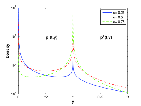
Figure 1: (Color online) The probability density $p^{-}(y)$ with support on $0<y<t$ and the density $p^{+}(y)$ with support on $y>t$ for different values of the index $\alpha$.

III Anomalous diffusion with under- and overshooting subordination

According to wjmwt2010 , the widely observed fractional two-power relaxation dependencies

$$\chi(\omega)\sim\left(i\omega/\omega_{p}\right)^{n-1}\quad{\rm for}\quad\omega\gg\omega_{p}$$ (11)

and

$$\Delta\chi(\omega)\sim\left(i\omega/\omega_{p}\right)^{m}\quad{\rm for}\quad\omega\ll\omega_{p}$$ (12)

of the complex susceptibility $\chi(\omega)=\chi^{\prime}(\omega)-i\chi^{\prime\prime}(\omega)$, where $\Delta\chi(\omega)=\chi(0)-\chi(\omega)$, the exponent $n$ and $m$ fall in the range $(0,1)$, and $\omega_{p}$ denotes the loss peak frequency, are closely connected with the under- and overshooting subordination

$$Z^{U}_{\alpha,\gamma}(t)<S_{\alpha}(t)<Z^{O}_{\alpha,\gamma}(t)\quad{\rm for}\quad t>0\,,$$

where $Z^{U}_{\alpha,\gamma}(t)=X^{U}_{\gamma}[S_{\alpha}(t)]$, $Z^{O}_{\alpha,\gamma}(t)=X^{O}_{\gamma}[S_{\alpha}(t)]$. Here the processes $X^{U}_{\gamma}(t)$ and $X^{O}_{\gamma}(t)$ are nothing else as $T^{-}_{S_{t}}$ and $T_{S_{t}}$ with the index $\gamma$. They are subordinated by an independent inverse $\alpha$-stable process $S_{\alpha}(t)$ forming the compound subordinators $Z^{U}_{\alpha,\gamma}(t)$ and $Z^{O}_{\alpha,\gamma}(t)$, respectively. The approach enlarges the class of diffusive scenarios in the framework of the CTRWs. This new type of coupled CTRWs follows from the clustering-jump random walks idea vlad . As it has been rigorously proved urlew05 , the clustering with finite-mean-value cluster sizes leads to the classical decoupled CTRW models, but assuming a heavy-tailed cluster-size distribution with the tail exponent $0<\gamma<1$, the coupling between jumps and interjump times tends to the compound operational times $Z^{U}_{\alpha,\gamma}(t)$ and $Z^{O}_{\alpha,\gamma}(t)$ as under- and overshooting subordinators, respectively.

The overshooting subordinator yields the anomalous diffusion scenario leading to the well-known Havriliak-Negami relaxation pattern J , and the undershooting subordinator leads to a new relaxation law given by the generalized Mittag-Leffler relaxation function jwt2008 ; wjmwt2010 . These results are in agreement with the idea of a superposition of the classical (exponential) Debye relaxations. Thus, the stochastic mechanism underlying the anomalous relaxation is quite clear, but the corresponding diffusion analysis requires some additional clarity. Let $B(t)$ be the parent process that is subordinated either by $Z^{U}_{\alpha,\gamma}(t)$ or $Z^{O}_{\alpha,\gamma}(t)$. Then the subordination relation, expressed by means of a mixture of pdf’s, takes the form

$$p^{\,r}(x,t)=\int_{0}^{\infty}\int_{0}^{\infty}p^{B}(x,y)\,p^{\pm}(y,\tau)\,p^{S}(\tau,t)\,dy\,d\tau\,,$$ (13)

where $p^{\,r}(x,t)$ is the probability density of the subordinated process $B[Z^{U}_{\alpha,\gamma}(t)]$ (or $B[Z^{O}_{\alpha,\gamma}(t)]$) with respect to the coordinate $x$ and time $t$, $p^{B}(x,\tau)$ the probability density of the parent process, $p^{\pm}(y,\tau)$ the probability density of $T^{-}_{S_{t}}$ and $T_{S_{t}}$ respectively, and $p^{S}(\tau,t)$ the probability density of $S(t)$. Recall that for the subdiffusion $B[S(t)]$, by taking the Laplace transform from the corresponding subordination relation, we can derive the celebrated fractional Fokker-Planck equation km2000 . It is therefore reasonable to ask is it possible to find a diffusion equation corresponding to relation (13). In the Laplace space

$$\bar{f}(u)=\int^{\infty}_{0}e^{-ut}\,f(t)\,dt$$

we obtain

$$\bar{p}^{\,r}(x,u)=u^{\alpha-1}\int_{1}^{\infty}\bar{p}^{B}(x,u^{\alpha}/z)\,p^{+}_{0}(z)\,\frac{dz}{z}\\$$ (14)

with $p^{+}_{0}(z)=\sin(\pi\gamma)\,z^{-1}(z-1)^{-\gamma}/\pi$ for $z>1$, as well

$$\bar{p}^{\,r}(x,u)=u^{\alpha-1}\int_{0}^{1}\bar{p}^{B}(x,u^{\alpha}/z)\,p^{-}_{0}(z)\,\frac{dz}{z}$$ (15)

with $p^{-}_{0}(z)=\sin(\pi\gamma)\,z^{\gamma-1}(1-z)^{-\gamma}/\pi$ for $0<z<1$. The Laplace image of the pdf of the subordinated process $B[S(t)]$ can be simply expressed in terms of an algebraic form with the Laplace image of the parent process pdf. This allows one to get the fractional Fokker-Planck equation driving the spatio-temperal evolution of the propagator of the anomalous diffusion underlying the Mittag-Leffler relaxation magwer06 ; stan03 ; km2000 . However, expressions (14) and (15) are not similar to the latter. They have an integral form. Nevertheless, derivation of the corresponding Fokker-Planck equation is also possible.

If we take the Laplace transform with respect to $t$ and the Fourier transform with respect to $x$ for $p^{\,r}(x,t)$ in Eq. (13), the Fourier-Laplace (FL) image reads

$$\textbf{FL }(p^{\,r})(k,s)$$ (16)

$$= s^{\alpha-1}\int_{0}^{\infty}\int_{0}^{\infty}e^{-\psi(k)y}\,p^{\pm}(y,\tau)\,e^{-\tau s^{\alpha}}\,dy\,d\tau\,,$$

where $\psi(k)$ is the log-Fourier transform of the parent process pdf $p^{B}(x,y)$. Consider the case of $p^{-}(y,\tau)$. After changing variables $y=z\tau$ we take the integral

$$\int^{\infty}_{0}e^{-\tau(s^{\alpha}+\psi(k)z)}\,d\tau=\frac{1}{s^{\alpha}+\psi(k)z}\,.$$

Next, the change of variables $t=z/(1-z)$ maps $[0\,,\,1]$ onto $[0\,,\,\infty)$. This helps to derive

$$\textbf{FL }(p^{\,r})(k,s)=\frac{s^{\alpha-1}}{\Gamma(\gamma)\Gamma(1-\gamma)}\int^{\infty}_{0}\frac{t^{\gamma-1}\,dt}{(s^{\alpha}+\psi(k))t+s^{\alpha}}\,.$$

The last expression can be easily calculated from the integral abr64

$$\int^{\infty}_{0}\frac{t^{\gamma-1}}{t+1}\,dt=\Gamma(\gamma)\Gamma(1-\gamma)\,.$$

The FL image of $p^{\,r}(x,t)$ with the undershooting directing process $Z^{U}_{\alpha,\gamma}(t)=X^{U}_{\gamma}[S_{\alpha}(t)]$ is of the form

$$\textbf{FL }(p^{\,r})(k,s)=\frac{s^{\alpha\gamma-1}}{(s^{\alpha}+\psi(k))^{\gamma}}\,.$$ (17)

Finally, we invert the Fourier and Lapace transforms to get the pseudo-differential equation

$$\Bigg{[}\frac{\partial^{\alpha}}{\partial t^{\alpha}}+L_{\rm FP}(x)\Bigg{]}^{\gamma}\,p^{\,r}(x,t)=\delta(x)\frac{t^{-\alpha\gamma}}{\Gamma(1-\alpha\gamma)}\,,$$ (18)

where $L_{\rm FP}(x)$ is the Fokker-Planck operator, $\delta(x)$ the Dirac function, and $\partial^{\alpha}/\partial t^{\alpha}$ denotes the Riemann-Louiville derivative. The corresponding Fokker-Planck equation can be obtained also in the case when the overshooting directing process $Z^{O}_{\alpha,\gamma}(t)=X^{O}_{\gamma}[S_{\alpha}(t)]$ is taken into account. Unfortunately, the derivation is more complicated as we present below.

In the case of $p^{+}(y,\tau)$, after the substitution $y=z\tau$, we map $[1\,,\,\infty)$ onto $[0\,,\,1]$ by the change of variables $z=1/x$. Then we obtain the corresponding FL image

$$\textbf{FL }(p^{\,r})(k,s)=\frac{s^{\alpha-1}}{\Gamma(\gamma)\Gamma(1-\gamma)}\int^{1}_{0}\frac{x^{\gamma-1}\,(1-x)^{-\gamma}\,dt}{s^{\alpha}+\psi(k)/x}\,.$$

The mapping $t=x/(1-x)$ transforms the latter expression to the form

$$\textbf{FL }(p^{\,r})(k,s)$$

$$= \frac{s^{\alpha-1}}{\Gamma(\gamma)\Gamma(1-\gamma)}\int^{\infty}_{0}\frac{t^{\gamma}\,dt}{(1+t)[(s^{\alpha}+\psi(k))t+\psi(k)]}\,.$$

This integral can be calculated exactly:

$$\int^{\infty}_{0}\frac{t^{\gamma}}{(t+1)(at+b)}\,dt=\frac{\Gamma(\gamma)\Gamma(1-\gamma)}{(a-b)}\Big{[}1-(b/a)^{\gamma}\Big{]}\,.$$

As a result, the FL image of $p^{\,r}(x,t)$ with the directing process $Z^{O}_{\alpha,\gamma}(t)=X^{O}_{\gamma}[S_{\alpha}(t)]$, can be written as

$$\textbf{FL }(p^{\,r})(k,s)=\frac{1}{s}\Bigg{\{}1-\left(\frac{\psi(k)}{s^{\alpha}+\psi(k)}\right)^{\gamma}\Bigg{\}}\,.$$ (19)

Now we invert the Fourier and Laplace transforms to get the pseudo-differential equation

$$\Bigg{[}\frac{\partial^{\alpha}}{\partial t^{\alpha}}+L_{\rm FP}(x)\Bigg{]}^{\gamma}\,p^{\,r}(x,t)=f_{\alpha,\gamma}(x,t)\,,$$ (20)

where

$$f_{\alpha,\gamma}(x,t)=\Bigg{\{}\Bigg{[}\frac{\partial^{\alpha}}{\partial t^{\alpha}}+L_{\rm FP}(x)\Bigg{]}^{\gamma}-\Bigg{[}L_{\rm FP}(x)\Bigg{]}^{\gamma}\Bigg{\}}\,\delta(x)$$

is a function depending on the probability density $p^{B}(x,y)$. The exact form of $f_{\alpha,\gamma}(x,t)$ is quite different from the right-side term of Eq.(18). In this connection it should be pointed out the work kcct04 , where the derivation of a fractional Fokker-Planck underlying the Havriliak-Negami type of relaxation is based on the entirely phenomenological approach of nr97 . However, the stochastic background leading to the anomalous diffusion yielding the Havriliak-Negami pattern, has remained behind these works. It should be noticed that Eqs.(18) and (20) have been derived independently in papers MMOCTRW ; StuMath .

To calculate the moments of the processes $B[Z^{U}_{\alpha,\gamma}(t)]$ and $B[Z^{O}_{\alpha,\gamma}(t)]$, assume for simplicity, that the parent process $B$ is a one-dimensional Brownian motion. Its moments are written as

$$I_{2n}(t) = \frac{1}{\sqrt{4\pi Dt}}\int^{\infty}_{-\infty}x^{2n}\,\exp\Bigg{(}-\frac{x^{2}}{4Dt}\Bigg{)}\,dx$$

$$= \frac{(2n)!}{n!}\,(Dt)^{n}\,,$$

where $D$ is the diffusion coefficient. If the subordinator $Z^{U}_{\alpha,\gamma}(t)$ governs the Brownian motion, then the moment integral reads

$$<x^{2n}> = \int^{\infty}_{-\infty}x^{2n}\,p^{\,r}(x,t)\,dx$$ (21)

$$= B_{n}\int^{1}_{0}z^{n}\,p^{-}_{0}(z)\,dz\int_{0}^{\infty}\tau^{n}\,p^{S}(\tau,y)\,d\tau$$

$$= \frac{(2n)!}{n!}\,D^{n}\frac{(\gamma,n)}{n!}\frac{t^{n\alpha}}{\Gamma(1+n\alpha)}\,,$$

where $(\gamma,n)=\gamma(\gamma+1)(\gamma+2)\dots(\gamma+n-1)$ is the Appell’s symbol with $(\gamma,0)=1$. When another subordinator $Z^{O}_{\alpha,\gamma}(t)$ is used, even the first moment of the subordinated process $B[Z^{O}_{\alpha,\gamma}(t)]$ diverges because the probability density $p^{+}_{0}(z)$ gives no finite moments. Thus, the process $B[Z^{U}_{\alpha,\gamma}(t)]$ is subdiffusion, and $B[Z^{O}_{\alpha,\gamma}(t)]$ is superdiffusion. In Fig. 2, as an example, the propagator $p^{r}(x,t)$ for the under- and overshooting anomalous diffusion with $\alpha=2/3$ and $\gamma=2/3$ is drawn.

It should be noticed that the ordinary subdiffusion $B[S_{\alpha}(t)]$ takes an intermediate place between the under- and overshooting anomalous diffusion $B[Z^{U}_{\alpha,\gamma}(t)]$ and $B[Z^{O}_{\alpha,\gamma}(t)]$. The feature is illustrated in Fig. 3. This allows one to compare an asymptotic behavior of the temporal evolution of diffusion fronts. From that one can see that the diffusion front of $B[Z^{U}_{\alpha,\gamma}(t)]$ is more stretched than the front of $B[S_{\alpha}(t)]$, whereas the diffusion front of $B[Z^{O}_{\alpha,\gamma}(t)]$ is more contracted in comparison with the front of $B[S_{\alpha}(t)]$.

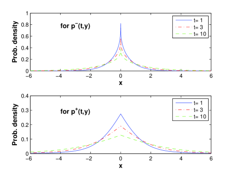
Figure 2: (Color online) Propagator $p^{r}(x,t)$ of the under- and overshooting anomalous diffusion with a constant potential, $\alpha=2/3$ and $\gamma=2/3$, drawn for consecutive dimensionless instances of time $t=1,3,10$. The cusp shape of the pdfs appears.

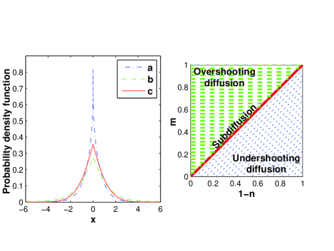
Figure 3: (Color online) Left panel: the propagator $p^{r}(x,t)$ of under- (a) and overshooting (b) anomalous diffusion with $\alpha=2/3$ and $\gamma=2/3$ for $t=1$. The line (c) displays the propagator of ordinary subdiffusion with $\alpha=2/3$ and $\gamma=1$ for $t=1$. Right panel: diagram shows the interrelation between $B[Z^{U}_{\alpha,\gamma}(t)]$, $B[S_{\alpha}(t)]$ and $B[Z^{O}_{\alpha,\gamma}(t)]$. Here $m$ and $1-n$ denote the power-law exponents defined in formulas (11) and (12).

One of interesting questions is what interpretation can be assigned to the subordinators $Z^{U}_{\alpha,\gamma}(t)=X^{U}_{\gamma}[S_{\alpha}(t)]$ and $Z^{O}_{\alpha,\gamma}(t)=X^{O}_{\gamma}[S_{\alpha}(t)]$. As the processes $X^{U}_{\gamma}(\tau)$ and $X^{O}_{\gamma}(\tau)$ are independent on $S_{\alpha}(t)$, they can be considered separately. The inverse Lévy-stable process $S_{\alpha}(t)$ accounts for the amount of time, when a walker does not participate in motion. The pdf of the subordinated process $B[X^{U}_{\gamma}(\tau)]$ is a special case of the Dirichlet average, namely

$$F(\gamma,x,\tau)=\frac{\sin\pi\alpha}{\pi}\int_{0}^{1}p^{B}(x,\tau z)\,z^{\gamma-1}\,(1-z)^{-\gamma}\,dz\,.$$

Recall that many of important special and elementary functions can be represented as Dirichlet averages of continuous functions (see more details in carlson ). The Dirichlet average includes the well-known means (arithmetic, geometric and others) as special cases. The process $X^{U}_{\gamma}(t)$ evolves to infinity like time $t$. Its contribution in the subordinated process $B[X^{U}_{\gamma}(t)]$ is taken into account by the Dirichlet average of the probability density of the parent process $B$. The similar reasoning can be developed for the process $X^{O}_{\gamma}(t)$.

IV Conclusions

The paper introduces an approach to study of the coupling between the very large jumps in physical and operational times. It is based on the compound subordination of a Lévy-stable process $T(\tau)$ by its inverse $S(t)$. The inverse Lévy-stable process is actually the left-inverse process of the Lévy-stable process. In fact, we have $S[T(\tau)]=\tau$, while $T[S(t)]>t$ holds. In the framework of CTRWs and the Langevin-type stochastic differential equations the compound subordinator provides a direct coupling of physical and operational times. The subordination scenario leads to two types of operational time: the spent life-time and the residual age. In the first random process all the moments are finite, whereas the second process has no finite moments. We have shown that the approach is useful for analysis of anomalous diffusion underlying all empirical fractional two-power-law relaxation responses. Due to the two types of the operational time the diffusion can display as well the subdiffusive and superdiffusive character.

References

- (1) R. Metzler and J. Klafter, J. Phys. A 37, R161(2004).
- (2) A.A. Stanislavsky, Theor. and Math. Phys. 138, 418(2004).
- (3) M. Magdziarz and K. Weron, Physica A 367, 1(2006).
- (4) P. Becker-Kern, M.M. Meerschaert, and H.-P. Scheffler, Ann. Probab. 32(1B), 730(2004).
- (5) M.M. Meerschaert, E. Scalas, Physica A 370, 114(2006).
- (6) A. Stanislavsky, Acta Phys. Polon. B 34(7), 3649(2003).
- (7) A. Weron, M. Magdziarz, and K. Weron, Phys. Rev. E 77, 036704(2008).
- (8) M. Magdziarz, A. Weron, and J. Klafter, Phys. Rev. Lett. 101, 210601(2008).
- (9) A. Jurlewicz, K. Weron, and M. Teuerle, Phys. Rev. E 78, 011103(2008).
- (10) K. Weron, A. Jurlewicz, M. Magdziarz, A. Weron, and J. Trzmiel, Phys. Rev. E 81, 041123(2010).
- (11) W. Feller, Introduction to probability theory and its application, Vol. II (John Wiley & Sons Inc., New York, 1967).
- (12) E.B. Dynkin, “Some limit theorems for sums of independent random variables with infinite mathematical expectation”, In: Selected Translations Math. Stat. Prob. 1, Inst. Math. Statistics Amer. Math. Soc., 171(1961).
-
(13)
J. Bertoin, “Subordinators, Lévy processes with no negative
jumps, and branching processes”, Lecture Notes Concentrated Adv.
Course Lévy Process 8, MaPhySto, University of Aarhus. http://www.maphysto.dk/oldpages/events/LevyBranch
2000/ - (14) T. Huillet, J. Phys. A 33, 2631(2000).
- (15) M.O. Vlad, Phys. Rev. A 45, 3600(1992); M.O. Vlad and M.C. Mackey, Phys. Rev. E 51, 3104(1995).
- (16) A. Jurlewicz, Diss. Math. 431, 1(2005).
- (17) A.K. Jonscher, Deilectric Relaxation in Solids, Chelsea Dielectrics Press, London, 1983.
- (18) R. Metzler and J. Klafter, Phys. Rep. 339, 1(2000).
- (19) M. Abramowitz and I.A. Stegun, Handbook of Mathematical Functions with Formulas, Graphs, and Mathematical Tables (Dover, New York, 1964).
- (20) Y.P. Kalmykov, W.T. Coffey, D.S.F. Crothers, and S.V. Titov, Phys. Rev. E 70, 041103(2004).
- (21) R.R. Nigmatullin and Ya.A. Ryabov, Phys. Solid State 39, 87(1997).
- (22) A. Jurlewicz, P. Kern, M.M. Meerschaert, and H.P. Scheffler, Comp. Math. App. (2011), doi:10.1016/j.camwa.2011.10.0100.
- (23) A. Jurlewicz, M.M. Meerschaert, and H.P. Scheffler, Studia Math. 205, 13(2011).
- (24) B.C. Carlson, Special Functions of Applied Mathematics (Academic Press, New York, 1977).