Renormalization-group calculation of the superfluid/normal-fluid
interface of liquid ⁴He in gravity near $T_{\lambda}$

Abstract

The superfluid/normal-fluid interface of liquid ⁴He is investigated in gravity on earth where a small heat current $Q$ flows vertically upward or downward. We present a local space- and time-dependent renormalization-group (RG) calculation based on model $F$ which describes the dynamic critical effects for temperatures $T$ near the superfluid transition $T_{\lambda}$. The model-$F$ equations are rewritten in a dimensionless renormalized form and solved numerically as partial differential equations. Perturbative corrections are included for the spatially inhomogeneous system within a self-consistent one-loop approximation. The RG flow parameter is determined locally as a function of space and time by a constraint equation which is solved by a Newton iteration. As a result we obtain the temperature profile of the interface. Furthermore we calculate the average order parameter $\langle\psi\rangle$, the correlation length $\xi$, the specific heat $C_{Q}$ and the thermal resistivity $\rho_{\mathrm{T}}$ where we observe a rounding of the critical singularity by the gravity and the heat current. We compare the thermal resistivity with an experiment and find good qualitative agreement. Moreover we discuss our previous approach for larger heat currents and the self-organized critical state and show that our theory agrees with recent experiments in this latter regime.

I Introduction

On earth in liquid ⁴He the gravity is an external force which causes a space dependent pressure $p=p(z)$ depending on the altitude coordinate $z$. Since the critical temperature of the superfluid transition $T_{\lambda}=T_{\lambda}(p)$ depends on the pressure $p$, in the helium the critical temperature $T_{\lambda}(z)=T_{\lambda}(p(z))$ varies with the altitude $z$. In leading approximation it is a linear function of the altitude

$$T_{\lambda}(z)=T_{\lambda}(z_{0})+(\partial T_{\lambda}/\partial z)\,(z-z_{0})$$ (1)

where the gradient is determined experimentally as Al68 $\partial T_{\lambda}/\partial z=+1.273\,\mathrm{\mu K/cm}$. The sign is positive which means that the critical temperature increases with the altitude $z$.

In thermal equilibrium, the local temperature of the helium $T(\mathbf{r},t)=T$ is constant with respect to any space and time variable. If in an experiment we choose the temperature $T=T_{\lambda}(z_{0})$ we find an interface at $z=z_{0}$, which separates superfluid ⁴He in the upper region $z>z_{0}$ where $T<T_{\lambda}(z)$ from normal-fluid ⁴He in the lower region $z<z_{0}$ where $T>T_{\lambda}(z)$. This interface is the main concern of the present paper.

Correlation effects imply an interface which is not sharply defined but smeared out over a certain length scale $\xi_{g}$. Ginzburg and Sobyanin GS76 have calculated the order parameter profile $\psi(z)$ for liquid ⁴He in gravity within their $\psi$ theory which is a mean-field theory modified by scaling functions in order to incorporate the effects of critical fluctuations and the critical exponents to some extent. They find the characteristic length scale $\xi_{g}=67\,\mathrm{\mu m}$ (see Fig. 4 and Eq. (3.49) in Ref. GS76, ).

A heat current $Q$ flowing from bottom to top in the direction of $z$ enhances the formation of the superfluid/normal-fluid interface. Heat transport phenomena imply a space-dependent temperature $T(z)$ with a negative gradient $\partial T/\partial z<0$ which acts opposed to the positive gradient of the critical temperature $T_{\lambda}(z)$. Onuki On83 ; On87 has investigated the interface under a heat flow $Q$ within a dynamic mean-field theory modified by scaling functions. He finds that the thickness of the interface decreases according to $\xi_{Q}\sim Q^{-1/2}$ with increasing heat current $Q$.

While on earth the gravity acceleration $g=9.81\,\mathrm{m/s^{2}}$ is constant, the heat current $Q$ can be varied in the experiment. For large heat currents $Q\gtrsim Q_{0}$, the heat-current effects dominate, where on the other hand for small heat currents $Q\lesssim Q_{0}$ gravity effects dominate. The heat current which separates both regimes, is about $Q_{0}=70\,\mathrm{nW/cm^{2}}$. In this paper we focus on small heat currents where gravity is the main effect.

The critical dynamics of liquid ⁴He near the superfluid transition $T_{\lambda}$ is described by a hydrodynamic model with Gaussian fluctuating forces which is called model $F$ in the classification of Hohenberg and Halperin HH77 . This model has originally been derived by Halperin, Hohenberg, and Siggia HHS74 in order to describe the critical dynamics of a planar ferromagnet, which is in the same universality class as liquid ⁴He. The field-theoretic renormalization-group theory of model $F$ has been elaborated by Dohm Do85 ; Do91 . The specific heat and the thermal conductivity have been calculated up to two-loop order Do85 and compared with very accurate experimental data Al84 ; Al85 . In this way, the renormalized coupling parameters and some other parameters have been adjusted Do91 so that all parameters of model $F$ are known. Thus model $F$ is ready for application without any further adjustable parameters.

In this paper we present a renormalization-group (RG) calculation of the superfluid/normal-fluid interface based on model $F$. The calculation is technically very difficult and challenging for two reasons. First the Green functions and Feynman diagrams must be evaluated in a spatially inhomogeneous system. Secondly, the renormalization factors depend on space and time coordinates via the RG flow parameter so that the partial derivatives with respect to space and time must be replaced by appropriate covariant derivatives.

The first challenge was overcome step by step in several previous papers. On the normal-fluid side of the interface the Green function was calculated HD91 for a zero order parameter $\langle\psi(z)\rangle=0$ and a linear temperature parameter $r_{0}(z)=a_{0}+b_{0}z$. The local thermal conductivity $\lambda_{T}(T,Q)$ and the related temperature profile $T(z)$ was calculated. On the superfluid side of the interface the Green function and related thermodynamic quantities were calculated HD92 for a plane-wave order parameter $\langle\psi(z)\rangle=\eta\,e^{ikz}$ and a constant temperature parameter $r_{0}$. Here a critical superfluid current was found which implies a depression of the superfluid transition temperature $T_{\lambda}(Q)<T_{\lambda}$ by a nonzero heat current $Q$.

Later the normal-fluid approach HD91 was extended beyond the interface into the superfluid region Ha99 ; Ha99a . The calculation was made self consistent by a lowest-order $1/n$ expansion which is equivalent to the Hartree approximation of quantum many-particle physics. In this way the superfluid region could be reached where in the whole system the average order parameter $\langle\psi(z)\rangle=0$ is zero due to phase fluctuations related to the motion of vortices where however the condensate density $n_{\mathrm{s}}=\langle|\psi(z)|^{2}\rangle$ and the superfluid current $\mathbf{J}_{\mathrm{s}}=\langle\mathrm{Im}[\psi^{*}\nabla\psi]\rangle$ are macroscopically large. The RG theory was applied locally using a local flow parameter which depends on the altitude coordinate $z$. The specific heat $C_{Q}$ and the thermal conductivity $\lambda_{T}$ were calculated for the whole superfluid/normal-fluid interface where the effects of the gravity acceleration $g$ and the heat current $Q$ were included. The temperature profile $T(z)$ was obtained by integrating the heat-transport equation $\mathbf{Q}=-\lambda_{T}\nabla T$.

In the superfluid region a nonzero temperature gradient $\nabla T$ was found which is due to a nonzero thermal resistivity induced by the motion of vortices and quantum turbulence. The theory was especially successful to describe the so called self-organized critical state, which was predicted by Onuki On87 and which was discovered in the experiment by Moeur et al. Du97 . In this state the temperature gradient $\nabla T$ is equal to the gravity induced gradient $\nabla T_{\lambda}$ of (1), i.e. $\nabla T=\nabla T_{\lambda}$, so that the system is homogeneous over a large area in space.

However, for the superfluid/normal-fluid interface the self-consistent approach Ha99 ; Ha99a works only for large heat currents $Q\gtrsim Q_{0}=70\,\mathrm{nW/cm^{2}}$ where the heat current $Q$ dominates over the effects of gravity $g$. For smaller heat currents this approach does not yield a result. The existence and motion of vortices is essential for phase fluctuations in order to have a zero average order parameter $\langle\psi(z)\rangle=0$.

For small heat currents $Q\lesssim Q_{0}=70\,\mathrm{nW/cm^{2}}$ vortices are not present so that the average order parameter $\langle\psi(z)\rangle$ is nonzero. In this case, a local calculation is not possible. Instead, the full model-$F$ equations must be solved as partial differential equations. Here the second challenge arises if the RG theory is involved. The RG flow parameter is determined locally by a constraint condition so that it will depend on space and time. This fact requires the definition of covariant differential operators. A first step for this kind of theory was made by the author and Nikodem HN08 . The interface was investigated in thermal equilibrium where only the gravity acceleration $g$ is present but no heat current. The covariant derivatives were defined for the renormalized order parameter and for the renormalized temperature parameter. The renormalized Ginzburg-Landau equation was solved numerically as a boundary value problem by the multiple-shooting algorithm. Results for the order-parameter profile $\langle\psi(z)\rangle$, the correlation length $\xi$, and the heat capacity $C$ were obtained. However, the calculations HN08 were not finished and not published.

The present paper is devoted to continue, extend, and publish our recent calculations HN08 . We develop a local and time-dependent RG theory for small heat currents $Q\lesssim Q_{0}=70\,\mathrm{nW/cm^{2}}$ in order to fill the gap which our previous theory Ha99 ; Ha99a has left. We solve the partial differential equations of model $F$ together with a local constraint condition for the RG flow parameter. We calculate the average order parameter profile $\langle\psi(z)\rangle$ and the temperature profile $T(z)$ for the superfluid/normal-fluid interface. Furthermore, we calculate the related thermodynamic and transport quantities, i.e. the specific heat $C_{Q}$ and the thermal conductivity $\lambda_{T}$ or thermal resistivity $\rho_{T}=1/\lambda_{T}$. The calculations are not restricted to a stationary state of a constant heat current $Q$. More generally, we solve the model-$F$ equations as time-dependent partial differential equations, so that time-dependent and transient effects can be handled like the propagation of second sound.

The paper is organized as follows. In Sec. II we briefly describe model $F$, the reduced hydrodynamic model for the critical dynamics of liquid ⁴He near the superfluid transition. Furthermore, we explain the approximations that we use. In Sec. III we develop our method in order to solve the model-$F$ equations together with local constraint conditions for the local RG theory. In Sec. IV we present our numerical results for the superfluid/normal-fluid interface in gravity where small heat currents are flowing upward or downward. We compare our results with the experiment of Chatto et al. Du07 and find good agreement for the local thermal resistivity. In Sec. V we compare our small-heat-current results with the large-heat-current results of our previous approach Ha99 ; Ha99a . We discuss the stability of the solutions of our present and our previous approach. Finally, in Sec. VI we compare our present and our previous approach with other theories and recent experiments. We discuss and conclude to which extent our theory can describe mutual friction effects for larger heat currents due to the motion of vortices and quantum turbulence.

II Model and approximation

The local thermodynamic properties of liquid ⁴He are described by the three standard hydrodynamic variables, the mass density $\rho(\mathbf{r},t)$, the mass-current density $\mathbf{j}(\mathbf{r},t)$, and the entropy density $\sigma(\mathbf{r},t)$. Since ⁴He becomes superfluid below the critical temperature $T_{\lambda}\approx 2\,K$, there exists an additional fourth hydrodynamic variable, the macroscopic wave function $\psi(\mathbf{r},t)$, which is the order parameter of the superfluid phase transition. The full hydrodynamic equations for superfluid ⁴He described by all these four variables have been derived long ago by Pitaevski Pi59 .

For the critical dynamics near $T_{\lambda}$ the mass density $\rho$ and the mass-current density $\mathbf{j}$ are irrelevant variables, because the related hydrodynamic modes, first sound and viscosity effects, are fast. $\rho$ and $\mathbf{j}$ can be eliminated or integrated out, so that the remaining relevant variables for the critical slow modes near the transition (second sound and order parameter relaxation) are the order parameter $\psi$ and the entropy density $\sigma$. For these two relevant variables, the hydrodynamic equations are given by model $F$ HH77 and read

$$\frac{\partial\psi}{\partial t} = -2\Gamma_{0}\frac{\delta H}{\delta\psi^{*}}+ig_{0}\,\psi\frac{\delta H}{\delta m}+\theta_{\psi}\ ,$$ (2)

$$\frac{\partial m}{\partial t} = \lambda_{0}\nabla^{2}\frac{\delta H}{\delta m}-2g_{0}\,\mathrm{Im}\Bigl{(}\psi^{*}\frac{\delta H}{\delta\psi^{*}}\Bigr{)}+\theta_{m}\ .$$ (3)

For convenience and historical reasons, the dimensionless entropy density is denoted by $m=\sigma/k_{\mathrm{B}}$. In the equations

$$H = \ \int d^{d}r\,\bigl{[}\textstyle{\frac{1}{2}}\tau_{0}|\psi|^{2}+\textstyle{\frac{1}{2}}|\nabla\psi|^{2}+\tilde{u}_{0}|\psi|^{4}$$ (4)

$$\hskip 34.1433pt+\textstyle{\frac{1}{2}}\chi_{0}^{-1}m^{2}+\gamma_{0}m|\psi|^{2}-h_{0}m\bigr{]}$$

is the free energy functional divided by $k_{B}T$. The Gaussian stochastic forces $\theta_{\psi}$ and $\theta_{m}$ incorporate the fluctuations. They are defined by the averages $\langle\theta_{\psi}\rangle=0$, $\langle\theta_{m}\rangle=0$, and by the correlations

$$\langle\theta_{\psi}(\mathbf{r},t)\theta^{*}_{\psi}(\mathbf{r}^{\prime},t^{\prime})\rangle = 4\,\Gamma_{0}\,\delta(\mathbf{r}-\mathbf{r}^{\prime})\,\delta(t-t^{\prime})\ ,$$ (5)

$$\langle\theta_{m}(\mathbf{r},t)\theta_{m}(\mathbf{r}^{\prime},t^{\prime})\rangle = -2\,\lambda_{0}\,\nabla^{2}\,\delta(\mathbf{r}-\mathbf{r}^{\prime})\,\delta(t-t^{\prime})\ .\qquad$$ (6)

The dimension of the space $d$ is assumed to be arbitrary and continuous in the general calculations. However, eventually we set $d=3$ when evaluating explicit results for liquid ⁴He in a three-dimensional cell. For the calculations in the critical regime the model-$F$ equations (2)-(4) are treated by field-theoretic means, i.e. perturbation series expansion with respect to Feynman diagrams, renormalization, and the renormalization group. For example, the heat capacity and the thermal conductivity were evaluated up to two-loop order Do85 .

In this paper, we use an approximation following our previous work Ha99 ; Ha99a . In many-particle physics this approximation is known as the Hartree approximation (see e.g. Ref. FW71, ). It is a self-consistent approximation including only a single one-loop diagram which is the tadpole diagram. Alternatively, the approximation is obtained by the $1/n$ expansion in leading order, where $n$ is the number of complex fields in a generalized model with a generalized order parameter $\Psi=(\psi_{1},\ldots,\psi_{n})$.

For the model-$F$ equations (2) and (3) the approximation is obtained by taking the nonequilibrium average $\langle\cdots\rangle$ for all terms and by performing appropriate factorizations of the averages of products of the fluctuating hydrodynamic variables $\psi$, $\psi^{*}$, and $m$. The factorizations are justified by inspection of the Feynman diagrams of the Hartree approximation which are shown in Fig. 2 of Ref. Ha99a, . We factorize the nonlinear terms according to

$$2\Bigl{\langle}\frac{\delta H}{\delta\psi^{*}}\Big{\rangle} \approx \bigl{[}\tau_{0}-\nabla^{2}+4\tilde{u}_{0}\langle|\psi|^{2}\rangle+2\gamma_{0}\langle m\rangle\bigr{]}\langle\psi\rangle\ ,\qquad$$ (7)

$$\Bigl{\langle}\psi\frac{\delta H}{\delta m}\Big{\rangle} \approx \langle\psi\rangle\,\Bigl{\langle}\frac{\delta H}{\delta m}\Big{\rangle}\ ,$$ (8)

where

$$\Bigl{\langle}\frac{\delta H}{\delta m}\Big{\rangle}=\chi_{0}^{-1}\langle m\rangle+\gamma_{0}\langle|\psi|^{2}\rangle-h_{0}\ .$$ (9)

Without an approximation we obtain

$$-2\,\Bigl{\langle}\mathrm{Im}\Bigl{(}\psi^{*}\frac{\delta H}{\delta\psi^{*}}\Bigr{)}\Bigr{\rangle}=\nabla\langle\mathrm{Im}[\psi^{*}\nabla\psi]\rangle\ .$$ (10)

Consequently, from (2) and (3) we obtain the approximate equations

$$\frac{\partial\langle\psi\rangle}{\partial t} = -\Gamma_{0}\bigl{[}\tau_{0}-\nabla^{2}+4\tilde{u}_{0}n_{\mathrm{s}}+2\gamma_{0}\langle m\rangle\bigr{]}\langle\psi\rangle$$ (11)

$$+ig_{0}\bigl{[}\chi_{0}^{-1}\langle m\rangle+\gamma_{0}n_{\mathrm{s}}-h_{0}\bigr{]}\langle\psi\rangle\ ,$$

$$\frac{\partial\langle m\rangle}{\partial t} = \lambda_{0}\nabla^{2}\bigl{[}\chi_{0}^{-1}\langle m\rangle+\gamma_{0}n_{\mathrm{s}}-h_{0}\bigr{]}+g_{0}\,\nabla\mathbf{J}_{\mathrm{s}}\ ,\qquad$$ (12)

where we define the condensate density $n_{\mathrm{s}}$ and the superfluid current density $\mathbf{J}_{\mathrm{s}}$ by

$$n_{\mathrm{s}} = \langle|\psi|^{2}\rangle\ ,$$ (13)

$$\mathbf{J}_{\mathrm{s}} = \langle\mathrm{Im}[\psi^{*}\nabla\psi]\rangle\ ,$$ (14)

respectively.

Next, for convenience and simplification of the equations we define the temperature parameters

$$\Delta r_{0} = 2\chi_{0}\gamma_{0}\,\Bigl{\langle}\frac{\delta H}{\delta m}\Big{\rangle}$$ (15)

$$= 2\chi_{0}\gamma_{0}\,\bigl{[}\chi_{0}^{-1}\langle m\rangle+\gamma_{0}n_{\mathrm{s}}-h_{0}\bigr{]}\ ,$$

$$r_{0} = \tau_{0}+2\chi_{0}\gamma_{0}h_{0}+\Delta r_{0}$$ (16)

$$= \tau_{0}+2\chi_{0}\gamma_{0}\,\bigl{[}\chi_{0}^{-1}\langle m\rangle+\gamma_{0}n_{\mathrm{s}}\bigr{]}\ ,$$

and the modified temperature parameter

$$r_{1}=r_{0}+4u_{0}n_{\mathrm{s}}\ ,$$ (17)

where $u_{0}=\tilde{u}_{0}-\frac{1}{2}\chi_{0}\gamma_{0}^{2}$ is a combined coupling constant following Ref. Do85, . Thus, the model-$F$ equations can be written in the simple form

$$\frac{\partial\langle\psi\rangle}{\partial t} = -\Gamma_{0}\bigl{[}r_{1}-\nabla^{2}\bigr{]}\langle\psi\rangle+i\frac{g_{0}}{2\chi_{0}\gamma_{0}}\Delta r_{0}\langle\psi\rangle\ ,\qquad$$ (18)

$$\frac{\partial\langle m\rangle}{\partial t} = -\nabla\mathbf{q}\ .$$ (19)

The last equation is the heat transport equation where $\langle m\rangle=\langle\sigma\rangle/k_{\mathrm{B}}$ is the dimensionless entropy density and

$$\mathbf{q}=-\frac{\lambda_{0}}{2\chi_{0}\gamma_{0}}\nabla\Delta r_{0}-g_{0}\mathbf{J}_{\mathrm{s}}$$ (20)

is the dimensionless entropy current density. The latter is related to the heat current $\mathbf{Q}$ in standard physical units by $\mathbf{q}=\mathbf{Q}/k_{\mathrm{B}}T\approx\mathbf{Q}/k_{\mathrm{B}}T_{\lambda}$.

The order-parameter equation (18) can be written in the form $L\langle\psi\rangle=0$ where the operator $L$ is defined in (3.13) of our previous paper Ha99a and related to the off-diagonal matrix elements of the inverse Green function. This observation shows that the factorizations of the present approach are equivalent to the self-consistent approximation in our previous paper. We note that the factorization is applied only in the order parameter equation (18). The heat transport equation (19) is derived without any factorization or approximation.

The parameters $\Delta r_{0}$ and $r_{0}$ are related to the local space and time dependent temperature $T=T(\mathbf{r},t)$ and to the critical temperature $T_{\lambda}=T_{\lambda}(z)$ of (1) according to

$$\Delta r_{0} = 2\chi_{0}\gamma_{0}\,\Bigl{\langle}\frac{\delta H}{\delta m}\Big{\rangle}=2\chi_{0}\gamma_{0}\,\frac{T-T_{0}}{T_{\lambda}}\ ,\qquad$$ (21)

$$r_{0}-r_{0\mathrm{c}} = 2\chi_{0}\gamma_{0}\,\frac{T-T_{\lambda}}{T_{\lambda}}\ ,$$ (22)

where $T_{0}$ is a constant reference temperature. These equations have been derived in our previous paper Ha99a . The critical value of $r_{0}$ is $r_{0\mathrm{c}}=0$ in one-loop approximation Do85 and hence also in our self-consistent approximation. The factor $T_{\lambda}$ in the denominators is easily explained. Since $H$ is the free energy divided by $k_{\mathrm{B}}T_{\lambda}$ and since $m$ is the entropy density divided by $k_{\mathrm{B}}$, we find that the functional derivative $\delta H/\delta m$ is a temperature divided by $T_{\lambda}$. We note that the critical temperature $T_{\lambda}=T_{\lambda}(z)$ defined in (1) depends on the altitude $z$. Since the gradient is very small, the $z$ dependence is very weak. Thus, in the denominator we may approximately use a constant average value which may be the critical temperature at the interface $z=z_{0}$, i.e. $T_{\lambda}=T_{\lambda}(z)\approx T_{\lambda}(z_{0})$.

Until now, the condensate density $n_{\mathrm{s}}$ and the superfluid current density $\mathbf{J}_{\mathrm{s}}$ defined in (13) and (14) are unknown. Since they are defined by an average of two fields $\psi$ and $\psi^{*}$ they are related to the equal-time Green function

$$G(\mathbf{r},t;\mathbf{r}^{\prime},t) = \langle\psi(\mathbf{r},t)\psi^{*}(\mathbf{r}^{\prime},t)\rangle$$ (23)

$$= \langle\psi(\mathbf{r},t)\rangle\,\langle\psi^{*}(\mathbf{r}^{\prime},t)\rangle$$

$$+\langle\delta\psi(\mathbf{r},t)\delta\psi^{*}(\mathbf{r}^{\prime},t)\rangle\ .$$

This Green function was evaluated in the Appendix of Ref. Ha99a, . However, while in our previous paper the average order parameter $\langle\psi\rangle$ was zero, in the present paper it is nonzero. Hence, we must split the Green function into two contributions, a mean-field term and a fluctuating term where $\delta\psi=\psi-\langle\psi\rangle$ is the fluctuating field. While the mean-field term is expressed in terms of the average order parameter $\langle\psi\rangle$, the fluctuating term is given by the result of our previous paper. Consequently, the condensate density $n_{\mathrm{s}}$ and the superfluid current density $\mathbf{J}_{\mathrm{s}}$ are split into two contributions, too. From Eq. (3.24) and (3.25) of Ref. Ha99a, we obtain

$$n_{\mathrm{s}} = |\langle\psi\rangle|^{2}-\frac{2}{\varepsilon}A_{d}\,\Phi_{-1+\varepsilon/2}(X)\,r_{1}^{1-\varepsilon/2}\ ,$$ (24)

$$\mathbf{J}_{\mathrm{s}} = \mathrm{Im}[\langle\psi^{*}\rangle\nabla\langle\psi\rangle]$$ (25)

$$+\frac{g_{0}}{2\Gamma_{0}^{\prime}}\frac{\nabla\Delta r_{0}}{2\chi_{0}\gamma_{0}}\,\frac{1}{\varepsilon}A_{d}\,\Bigl{(}1-\frac{\varepsilon}{2}\Bigr{)}\,\Phi_{\varepsilon/2}(X)\,r_{1}^{-\varepsilon/2}\ .\qquad$$

Here it is $\varepsilon=4-d$ where $d$ is the dimension of the space. Furthermore, $A_{d}=S_{d}\,\Gamma(1-\varepsilon/2)\Gamma(1+\varepsilon/2)$ is a geometrical factor which is related via $S_{d}=\Omega_{d}/(2\pi)^{d}$ to the surface of the $d$ dimensional unit sphere $\Omega_{d}=2\,\pi^{d/2}/\Gamma(d/2)$. The function $\Phi_{\alpha}(X)$ is defined by the divergent series

$$\Phi_{\alpha}(X)=\sum_{N=0}^{\infty}\frac{\Gamma(\alpha+3N)}{\Gamma(\alpha)}\,\frac{X^{N}}{N!}$$ (26)

where the argument $X$ is related to the square of the gradients of the parameters $r_{1}$ and $\Delta r_{0}$ according to

$$X = \frac{1}{12\,r_{1}^{3}}\Bigl{[}(\nabla r_{1})^{2}+2\frac{\Gamma_{0}^{\prime\prime}}{\Gamma_{0}^{\prime}}\Bigl{(}\frac{g_{0}}{4\chi_{0}\gamma_{0}\Gamma_{0}^{\prime}}\nabla\Delta r_{0}\Bigr{)}\cdot\nabla r_{1}$$ (27)

$$-\Bigl{(}\frac{g_{0}}{4\chi_{0}\gamma_{0}\Gamma_{0}^{\prime}}\nabla\Delta r_{0}\Bigr{)}^{2}\Bigr{]}\ .$$

The Green function (23) was evaluated locally for a spatial inhomogeneous system where the temperature parameters $r_{1}$ and $\Delta r_{0}$ depend on the space coordinate $\mathbf{r}$. Gradient terms $\nabla r_{1}$ and $\nabla\Delta r_{0}$ are included but curvature terms and higher derivatives are omitted. This fact is clearly seen in the function (26) and its argument (27).

Now, all quantities are determined. The approximate model-$F$ equations (18)-(19) together with the entropy current density (20), the temperature parameters (21), (22), (17), and the quantities (24)-(27) are closed equations, which in principle can be solved numerically. We insert the condensate density (24) into the equation for the modified temperature parameter (17). After reordering the terms we obtain

$$r_{1}\Bigl{\{}1+8u_{0}\frac{1}{\varepsilon}A_{d}\,\Phi_{-1+\varepsilon/2}(X)\,r_{1}^{-\varepsilon/2}\Bigr{\}}=r_{0}+4u_{0}|\langle\psi\rangle|^{2}\ .$$ (28)

The left-hand side shows clearly that this is an implicit equation for the parameter $r_{1}$. Furthermore, we insert the superfluid current (25) into the formula for the entropy current (20). After reordering the terms we obtain

$$\mathbf{q} = -\frac{\lambda_{0}}{2\chi_{0}\gamma_{0}}\Bigl{\{}1+\frac{g_{0}^{2}}{2\lambda_{0}\Gamma_{0}^{\prime}}\frac{1}{\varepsilon}A_{d}\,\Bigl{(}1-\frac{\varepsilon}{2}\Bigr{)}\,\Phi_{\varepsilon/2}(X)\,r_{1}^{-\varepsilon/2}\Bigr{\}}$$ (29)

$$\times\nabla\Delta r_{0}-g_{0}\mathrm{Im}[\langle\psi^{*}\rangle\nabla\langle\psi\rangle]\ .$$

Eqs. (28) and (29) of the present paper should be compared with Eqs. (3.32) and (3.35) of our previous paper Ha99a , respectively. New contributions are those terms on the right hand sides which involve the average order parameter $\langle\psi\rangle$. The last term in (29) may be interpreted as the mean-field contribution of the superfluid current. The fluctuating term of the superfluid current (25) is proportional to the temperature-parameter gradient $\nabla\Delta r_{0}$. For this reason, the fluctuating term is integrated into the first term of (29) and hence contributes to the normal-fluid term. Similarly, in Eq. (28) the mean-field contribution of the condensate density is put on the right-hand side while the fluctuating contribution is put on the left-hand side of the equation.

III Local renormalization-group theory for partial differential equations

The liquid ⁴He is considered in the critical regime for temperatures $T$ close to the superfluid transition at $T_{\lambda}$. In order to treat the critical fluctuations correctly, we must renormalize the equations of the previous section and apply the renormalization-group (RG) theory. Since we consider local physical quantities which are functions of space and time, the RG flow parameter will be local and depend on space and time. The derivatives with respect to space and time in the model-$F$ equations are in conflict with a local RG flow parameter because they do not commute with this parameter. For this reason, the development of the local RG theory for the model-$F$ equations which are partial differential equations is a very challenging task.

III.1 Renormalization

We start with the renormalization of the average order parameter $\langle\psi\rangle$, the temperature parameters $\Delta r_{0}$, $r_{0}$, and the coupling constant $u_{0}$. Following Ref. Do85, we have

$$\langle\psi\rangle = Z_{\phi}^{1/2}\langle\psi_{\mathrm{ren}}\rangle\ ,$$ (30)

$$\Delta r_{0} = Z_{r}\,\Delta r\ ,$$ (31)

$$r_{0}-r_{0\mathrm{c}} = Z_{r}\,r\ ,$$ (32)

$$u_{0} = Z_{u}Z_{\phi}^{-2}(\mu^{\varepsilon}/A_{d})\,u\ .$$ (33)

In these and the following renormalization equations we use the convention that the bare quantities are always on the left-hand side while renormalized quantities are always on the right hand side. The $Z$ factors are the renormalization factors. In the Hartree approximation, which we use in the present paper and in our previous paper Ha99a , these $Z$ factors are

$$Z_{\phi}=1\ ,\qquad Z_{r}=Z_{u}=1/[1-8u/\varepsilon]\ ,$$ (34)

where it is $r_{0\mathrm{c}}=0$. The modified temperature parameter $r_{1}$ is not renormalized. We apply the renormalizations to Eq. (28), multiply both sides with the inverse factor $Z_{r}^{-1}$, and reorder the terms. Without any further approximation we obtain

$$r_{1}\Bigl{\{}1+\frac{8u}{\varepsilon}\Bigl{[}\Phi_{-1+\varepsilon/2}(X)\,\Bigl{(}\frac{r_{1}}{\mu^{2}}\Bigr{)}^{-\varepsilon/2}-1\Bigr{]}\Bigr{\}}$$

$$=r+4u\frac{\mu^{\varepsilon}}{A_{d}}|\langle\psi\rangle|^{2}\ .$$ (35)

The average entropy density $\langle m\rangle$, the entropy current density $\mathbf{q}$, and the remaining model-$F$ parameters are renormalized by Do85

$$\langle m\rangle = (\chi_{0}Z_{m})^{1/2}\,\langle m_{\mathrm{ren}}\rangle\ ,$$ (36)

$$\mathbf{q} = (\chi_{0}Z_{m})^{1/2}\,\mathbf{q}_{\mathrm{ren}}\ ,$$ (37)

$$\chi_{0}\gamma_{0} = (\chi_{0}Z_{m})^{1/2}Z_{r}(\mu^{\varepsilon}/A_{d})^{1/2}\,\gamma\ ,$$ (38)

$$g_{0} = (\chi_{0}Z_{m})^{1/2}(\mu^{\varepsilon}/A_{d})^{1/2}\,g\ ,$$ (39)

$$\lambda_{0}/\chi_{0} = Z_{\lambda}^{-1}\,\lambda\ ,$$ (40)

$$\Gamma_{0} = Z_{\Gamma}^{-1}\,\Gamma\ .$$ (41)

The dimensionless renormalized parameters are defined by the ratios

$$w = \Gamma/\lambda\ ,$$ (42)

$$F = g/\lambda\ ,$$ (43)

$$f = F^{2}/w^{\prime}=g^{2}/\lambda\Gamma^{\prime}\ .$$ (44)

We note that $\Gamma=\Gamma^{\prime}+i\Gamma^{\prime\prime}$ and $w=w^{\prime}+iw^{\prime\prime}$ are complex parameters. The $Z$ factors, which we need explicitly in our calculation, are given in Hartree approximation Ha99a by

$$Z_{m}Z_{\lambda}=1/[1-f/2\varepsilon]\ ,\qquad Z_{\Gamma}=1\ .$$ (45)

The factor $\chi_{0}Z_{m}$ will cancel out in all our equations. Hence this latter factor is not needed explicitly. Applying the renormalizations to Eq. (29) we obtain the renormalized heat current

$$\mathbf{q}_{\mathrm{ren}} = -\frac{\lambda}{2\gamma}\Bigl{(}\frac{A_{d}}{\mu^{\varepsilon}}\Bigr{)}^{1/2}\Bigl{\{}1+\frac{f}{2\varepsilon}\Bigl{[}\Bigl{(}1-\frac{\varepsilon}{2}\Bigr{)}$$ (46)

$$\times\Phi_{\varepsilon/2}(X)\Bigl{(}\frac{r_{1}}{\mu^{2}}\Bigr{)}^{-\varepsilon/2}-1\Bigr{]}\Bigr{\}}\,\nabla\Delta r$$

$$-g\,\Bigl{(}\frac{\mu^{\varepsilon}}{A_{d}}\Bigr{)}^{1/2}\mathrm{Im}[\langle\psi_{\mathrm{ren}}^{*}\rangle\nabla\langle\psi_{\mathrm{ren}}\rangle]\ .$$

Again no further approximation is made when reordering the terms. In order to evaluate the function $\Phi_{\alpha}(X)$ we need the argument $X$ expressed in terms of the dimensionless renormalized parameters. From (27) we obtain

$$X = \frac{1}{12\,r_{1}^{3}}\Bigl{[}(\nabla r_{1})^{2}+2\frac{w^{\prime\prime}}{w^{\prime}}\Bigl{(}\frac{F}{4\gamma w^{\prime}}\nabla\Delta r\Bigr{)}\cdot\nabla r_{1}$$ (47)

$$-\Bigl{(}\frac{F}{4\gamma w^{\prime}}\nabla\Delta r\Bigr{)}^{2}\Bigr{]}\ .$$

The renormalization of the model-$F$ equations is straight forward. From (18) and (19) we obtain

$$\frac{\partial\langle\psi_{\mathrm{ren}}\rangle}{\partial t} = -\Gamma\bigl{[}r_{1}-\nabla^{2}\bigr{]}\langle\psi_{\mathrm{ren}}\rangle+i\frac{g}{2\gamma}\Delta r\langle\psi_{\mathrm{ren}}\rangle\ ,\qquad$$ (48)

$$\frac{\partial\langle m_{\mathrm{ren}}\rangle}{\partial t} = -\nabla\mathbf{q}_{\mathrm{ren}}\ .$$ (49)

We furthermore need a relation between the entropy density $\langle m_{\mathrm{ren}}\rangle$ and the temperature parameters $r$ or $\Delta r$ in renormalized form. We solve Eq. (16) with respect to the entropy density $\langle m\rangle$, eliminate the condensate density $n_{\mathrm{s}}$ by (17), and then perform the renormalization. As a result we obtain

$$\langle m_{\mathrm{ren}}\rangle=m_{\mathrm{c,ren}}+\Bigl{(}\frac{A_{d}}{\mu^{\varepsilon}}\Bigr{)}^{1/2}\frac{r}{2\gamma}\Bigl{\{}1+\frac{\gamma^{2}}{2u}\Bigl{[}1-\frac{r_{1}}{r}\Bigr{]}\Bigr{\}}\ .$$ (50)

We have separated the constant value $m_{\mathrm{c,ren}}$ which is the entropy at the critical point with temperature $T=T_{\lambda}$, zero heat current $\mathbf{Q}=\mathbf{0}$ and zero gravity $g=0$. We need not know this constant value explicitly. Another useful quantity is the derivative of $\langle m_{\mathrm{ren}}\rangle$ with respect to the temperature parameter $r$. It is related to the renormalized specific heat Do85 according to

$$C_{\mathrm{ren}}=2\gamma\Bigl{(}\frac{\mu^{\varepsilon}}{A_{d}}\Bigr{)}^{1/2}\,\frac{\partial\langle m_{\mathrm{ren}}\rangle}{\partial r}=1+\frac{\gamma^{2}}{2u}\Bigl{[}1-\frac{\partial r_{1}}{\partial r}\Bigr{]}\ .$$ (51)

In this way, the time derivative of the renormalized entropy density can be expressed in terms of a time derivative of a temperature parameter. We find

$$\frac{\partial\langle m_{\mathrm{ren}}\rangle}{\partial t}=\frac{C_{\mathrm{ren}}}{2\gamma}\Bigl{(}\frac{A_{d}}{\mu^{\varepsilon}}\Bigr{)}^{1/2}\,\frac{\partial r}{\partial t}=\frac{C_{\mathrm{ren}}}{2\gamma}\Bigl{(}\frac{A_{d}}{\mu^{\varepsilon}}\Bigr{)}^{1/2}\,\frac{\partial\Delta r}{\partial t}\ .$$ (52)

Since the critical temperature $T_{\lambda}(z)$ does not depend on the time, the two temperature parameters $r$ and $\Delta r$ differ by a time-independent value. For this reason, the time derivatives of $r$ and $\Delta r$ are equal. In the present paper we prefer the latter time derivative. In this way, we reformulate the second model-$F$ equation (49) as

$$\frac{C_{\mathrm{ren}}}{2\gamma}\Bigl{(}\frac{A_{d}}{\mu^{\varepsilon}}\Bigr{)}^{1/2}\,\frac{\partial\Delta r}{\partial t}=-\nabla\mathbf{q}_{\mathrm{ren}}\ .$$ (53)

In the renormalized specific heat (51) the remaining derivative $\partial r_{1}/\partial r$ may be obtained as the proportionality factor of the gradients $\nabla r_{1}$ and $\nabla r$ according to

$$\nabla r_{1}=\frac{\partial r_{1}}{\partial r}\,\nabla r\ .$$ (54)

In order to find a relation between the two gradients we apply the nabla operator $\nabla$ to Eq. (35). Thus, we find

$$(\nabla r_{1})\Bigl{\{}1+\frac{8u}{\varepsilon}\Bigl{[}\Bigl{(}1-\frac{\varepsilon}{2}\Bigr{)}\Phi_{\varepsilon/2}(X)\,\Bigl{(}\frac{r_{1}}{\mu^{2}}\Bigr{)}^{-\varepsilon/2}-1\Bigr{]}\Bigr{\}}$$

$$=\nabla r+4u\frac{\mu^{\varepsilon}}{A_{d}}\,\nabla|\langle\psi_{\mathrm{ren}}\rangle|^{2}\ .$$ (55)

In this result the derivative has increased the index $\alpha$ of the function $\Phi_{\alpha}(X)$ by one. Furthermore, the function is multiplied by a factor $(1-\varepsilon/2)$. These facts are well known from the calculations in our previous paper Ha99a . By comparing Eqs. (54) and (55) we extract $\partial r_{1}/\partial r$. Since we consider the space dependence only in one dimension $z$ which is the altitude, we obtain a unique result. We conclude that in this subsection we have derived all equations in renormalized form which are needed for a numerical calculation to solve the model-$F$ equations as partial differential equations with respect to space and time.

III.2 Dimensionless renormalized quantities

In the renormalization equations (30)-(33) and (36)-(41) the new arbitrary parameter $\mu$ occurs which has the unit of an inverse length scale. Consequently, this parameter may be used to fix the length scale. On the other hand in the renormalized model-$F$ equations (48) and (53) together with (46) the dynamic parameters $\Gamma=\Gamma^{\prime}+i\Gamma^{\prime\prime}$, $\lambda$, and $g$ all have the unit of a diffusion constant, i.e. length square divided by time. Hence, these parameters multiplied by $\mu^{2}$ may be used to fix the time scale. The dimensionless ratios (42)-(44) imply that only one of these parameters is needed. Thus, we will use $g\mu^{2}$ to fix the time scale.

We rewrite the renormalized model-$F$ equations and the related renormalized variables and parameters in a dimensionless form using $\mu$ and $g\mu^{2}$ for the scales. Following our previous paper Ha99a we define the dimensionless temperature parameters

$$\Delta\rho = \Delta r/\mu^{2}=\tau^{-1}\,(T-T_{0})/T_{\lambda}\ ,$$ (56)

$$\rho = r/\mu^{2}=\tau^{-1}\,(T-T_{\lambda})/T_{\lambda}\ ,$$ (57)

$$\rho_{1} = r_{1}/\mu^{2}\ .$$ (58)

The last equality sign in (56) and (57) is obtained by renormalizing the bare equations (21) and (22). The renormalization factors are combined into the dimensionless parameter

$$\tau=\Bigl{(}\frac{A_{d}\mu^{d}}{\chi_{0}Z_{m}}\Bigr{)}^{1/2}\frac{1}{2\gamma}$$ (59)

which may be viewed as a renormalization-group (RG) flow parameter. A change of the length scale by replacing $\mu\to\mu\ell$ causes a change of $\tau$. While $\ell$ is the conventional RG flow parameter related to the length scale, $\tau=\tau(\ell)$ is a RG flow parameter related to the temperature scale. In the literature on the dynamic RG theory for liquid ⁴He both flow parameters have been used Do85 ; Do91 ; Ha99 ; Ha99a ; Ha99b . For the dimensionless coupling parameters of model $F$ the notations $u(\ell)$, $\gamma(\ell)$, etc. and $u[\tau]$, $\gamma[\tau]$, etc. have been used. In the present paper we will use $\tau$ as the RG flow parameter.

We define the dimensionless renormalized order parameter $Y$ and the dimensionless renormalized heat current $\tilde{\mathbf{q}}$ by

$$Y = \langle\psi_{\mathrm{ren}}\rangle/\mu^{(d-2)/2}\ ,$$ (60)

$$\tilde{\mathbf{q}} = \Bigl{(}\frac{A_{d}}{\mu^{\varepsilon}}\Bigr{)}^{1/2}\frac{\mathbf{q}_{\mathrm{ren}}}{g}\,\frac{1}{\mu^{d-1}}=\frac{\mathbf{q}}{g_{0}}\,\frac{1}{\mu^{d-1}}\ ,$$ (61)

respectively. For convenience of the notation, following Ref. Ha99a, we define the dimensionless amplitudes

$$A = \varepsilon^{-1}[\Phi_{-1+\varepsilon/2}(X)\,\rho_{1}^{-\varepsilon/2}-1]\ ,$$ (62)

$$A_{1} = \varepsilon^{-1}[(1-\varepsilon/2)\Phi_{\varepsilon/2}(X)\,\rho_{1}^{-\varepsilon/2}-1]\ .$$ (63)

Consequently, the renormalized heat current (46) can be rewritten in the dimensionless simple form

$$\tilde{\mathbf{q}}=\frac{1}{\mu}\Bigl{[}-\frac{A_{d}}{2\gamma F}\,\Bigl{\{}1+\frac{f}{2}A_{1}\Bigr{\}}\,\nabla\Delta\rho-\mathrm{Im}[Y^{*}\nabla Y]\Bigr{]}\ .$$ (64)

The overall factor $1/\mu$ is needed to keep the nabla operators dimensionless. We note that $A_{d}$ is a geometrical factor related to surface of the $d$ dimensional unit sphere Do85 . It should not be confused with the amplitudes $A$ and $A_{1}$. In an analogous way Eqs. (35) and (55) for the modified temperature parameter $\rho_{1}$ and its derivative $\nabla\rho_{1}$ can be written in a dimensionless form. We obtain

$$\rho_{1}\{1+8uA\} = \rho+(4u/A_{d})\,|Y|^{2}\ ,$$ (65)

$$(\nabla\rho_{1})\{1+8uA_{1}\} = \nabla\rho+(4u/A_{d})\,\nabla|Y|^{2}\ ,\qquad$$ (66)

where the second equation should be multiplied by an overall factor $1/\mu$ to make the nabla operators dimensionless. Finally, the renormalized specific heat $C_{\mathrm{ren}}$ defined in (51) and the parameter $X$ defined in (47) are already dimensionless, so that we can keep them unchanged. We must only insert the dimensionless temperature parameters (56)-(58) and use the dimensionless nabla operator $\mu^{-1}\nabla$.

Now, all variables and parameters are expressed in a dimensionless form. Thus, we are ready to rewrite the renormalized model-$F$ equations in dimensionless forms. From Eqs. (48) and (53) we obtain

$$\frac{1}{g\mu^{2}}\,\frac{\partial Y}{\partial t} = -\frac{w}{F}\bigl{[}\rho_{1}-\mu^{-2}\nabla^{2}\bigr{]}Y$$ (67)

$$+\frac{i}{2\gamma}\Delta\rho\,Y\ ,\qquad$$

$$\frac{C_{\mathrm{ren}}}{2\gamma}\frac{A_{d}}{g\mu^{2}}\,\frac{\partial\Delta\rho}{\partial t} = -\mu^{-1}\nabla\tilde{\mathbf{q}}\ ,$$ (68)

where $w=w^{\prime}+iw^{\prime\prime}$ is a complex parameter. In these equations we clearly see that $\mu$ defines the length scale and $g\mu^{2}$ defines the time scale. We may interpret $\mu^{-1}\nabla$ as a dimensionless nabla operator and $(g\mu^{2})^{-1}\partial/\partial t$ as a dimensionless time derivative.

III.3 Evaluation of the perturbative amplitudes

The amplitudes $A$ and $A_{1}$, defined in (62) and (63), respectively, represent the contributions of the perturbation series expansion which in our case is the Hartree term. In order to solve the model-$F$ equations as partial differential equations we must have explicit expression to evaluate these amplitudes. The non-trivial contribution in the amplitudes is the function $\Phi_{\alpha}(X)$ together with its variable $X$ which are defined in Eqs. (26) and (47). This function was first derived in Ref. HD91, . Unfortunately, the function is a divergent infinite series so that it is not well defined in this form. However, in thermal equilibrium at zero heat current $Q=0$ and zero gravity $g=0$ this function can be omitted because it is just unity. In this case all temperature gradients are zero, so that the variable $X$ is zero which implies $\phi_{\alpha}(X=0)=1$. Hence, the amplitudes reduce to

$$A = \varepsilon^{-1}[\rho_{1}^{-\varepsilon/2}-1]\ ,$$ (69)

$$A_{1} = \varepsilon^{-1}[(1-\varepsilon/2)\rho_{1}^{-\varepsilon/2}-1]\ .$$ (70)

Since $\rho_{1}\sim\rho\sim(T-T_{\lambda})$ must be positive, these amplitudes are valid for the normal-fluid equilibrium state only and agree with former results Do85 .

In the nonequilibrium state the variable $X$ is nonzero. In this case the infinite series (26) must be resummed to obtain a well-defined expression which can be evaluated numerically. Following our previous papers HD91 ; Ha99a we write

$$\Phi_{\alpha}(X)=[\Gamma(\alpha)]^{-1}\,\zeta^{\alpha}\,\mathcal{F}_{\alpha}(\zeta)$$ (71)

where $\zeta=(-X)^{-1/3}$ and

$$\mathcal{F}_{\alpha}(\zeta)=\int_{0}^{\infty}dv\,v^{\alpha-1}\,\exp(-v^{3}-v\zeta)\ .$$ (72)

The integral is well defined for $\alpha>0$ and obtained by analytical continuation for $\alpha<0$. The new variable $\zeta$ is defined by a third root. Consequently, $\zeta$ is not unique a priori and may be complex. We must specify the root which should be taken. For this purpose we define the dimensionless parameter

$$\sigma = -\frac{1}{12\,\mu^{2}}\Bigl{[}(\nabla\rho_{1})^{2}+2\frac{w^{\prime\prime}}{w^{\prime}}\Bigl{(}\frac{F}{4\gamma w^{\prime}}\nabla\Delta\rho\Bigr{)}\cdot\nabla\rho_{1}$$ (73)

$$-\Bigl{(}\frac{F}{4\gamma w^{\prime}}\nabla\Delta\rho\Bigr{)}^{2}\Bigr{]}\ .$$

so that $X=-\sigma/\rho_{1}^{3}$. Hence, the new variable can be written in the form $\zeta=\rho_{1}/\sigma^{1/3}$.

The transition from normal-fluid to superfluid ⁴He is related to a change of sign of $\rho_{1}\sim\rho\sim(T-T_{\lambda})$. Consequently, also the new variable $\zeta$ changes sign. The nontrivial third root to be evaluated is $\sigma^{1/3}$. For this reason, we must distinguish two cases which are related to the two possible signs of $\sigma$. This distinction has important physical consequences. There will be two kinds of nonequilibrium superfluid phases of liquid ⁴He which are related to the two regimes where either the heat current $Q$ or the gravity $g$ is the dominating external influence. We discuss these two cases in the following.

III.3.1 Heat current dominated regime: $\sigma>0$

The self-organized critical state observed in the experiment by Moeur et al. Du97 implies linear temperature profiles $T(z)$ and $T_{\lambda}(z)$ as function of the altitude $z$. The temperature difference $T(z)-T_{\lambda}(z)=\Delta T$ is constant over a large range of the altitude. Consequently, the related gradient parameters $\nabla\rho_{1}\sim\nabla\rho\sim\nabla(T-T_{\lambda})$ are zero. On the other hand the heat current $\mathbf{Q}$ causes a nonzero constant gradient $\nabla\Delta\rho\sim\nabla T$. Thus, in the formula (73) only the last term is nonzero which yields a positive result for $\sigma$. Hence, for the self-organized critical state the dimensionless parameter $\sigma$ is always constant and positive.

For the inhomogeneous nonequilibrium state we may conclude that $\sigma$ is also positive whenever the heat current $\mathbf{Q}$ and hence the related gradient $\nabla\Delta\rho$ is large compared to the effects of gravity. In our previous paper Ha99a we confirm $\sigma>0$ for heat transport in liquid ⁴He on earth for heat currents $Q\gtrsim 70\,\mathrm{nW/cm^{2}}$. Moreover, for an experiment in zero gravity conditions in space, $\sigma$ is positive for all heat currents.

Whenever $\sigma$ is positive, the root $\sigma^{1/3}$ is straight forward. We just take the real positive root. Consequently, the variable $\zeta$ is real and changes sign at the superfluid transition. We find $\zeta>0$ in the normal fluid regime and $\zeta<0$ is the superfluid regime. The function (71) and the integral (72) can be evaluated directly. As a result we obtain the amplitudes

$$A = \frac{1}{\varepsilon}\Bigl{[}\frac{\sigma^{-\varepsilon/6}}{\Gamma(-1+\varepsilon/2)}\,\zeta^{-1}\mathcal{F}_{-1+\varepsilon/2}(\zeta)-1\Bigr{]}\ ,\qquad$$ (74)

$$A_{1} = \frac{1}{\varepsilon}\Bigl{[}-\frac{\sigma^{-\varepsilon/6}}{\Gamma(-1+\varepsilon/2)}\,\mathcal{F}_{\varepsilon/2}(\zeta)-1\Bigr{]}\ ,$$ (75)

which we have derived and used in our previous paper Ha99a .

We investigate the asymptotic behaviors of the function $\mathcal{F}_{\alpha}(\zeta)$ and find

$$\mathcal{F}_{\alpha}(\zeta)\approx\Gamma(\alpha)\,\zeta^{-\alpha}$$ (76)

for $\zeta\gg+1$ in the normal-fluid regime and

$$\mathcal{F}_{\alpha}(\zeta)\approx(\pi/3)^{1/2}\,(-\zeta/3)^{\alpha/2-3/4}\,\exp\{2(-\zeta/3)^{3/2}\}$$ (77)

for $\zeta\ll-1$ in the superfluid regime, respectively Ha99a . In the first asymptotic case (76) we recover the amplitudes (69) and (70) of the normal-fluid equilibrium state. In the second asymptotic case (77) we obtain exponentially large amplitudes $A$ and $A_{1}$ for the nonequilibrium superfluid state.

The latter asymptotic case has an important physical consequence. We consider Eq. (65) which is a constraint to define $\rho_{1}$. In the original form related to (17) this equation is rewritten as

$$\rho_{1}=\rho-8uA\rho_{1}+(4u/A_{d})\,|Y|^{2}\ .$$ (78)

The last term is the contribution of the renormalized complex order parameter $Y$ which is nonzero only in the superfluid state. However, in the superfluid regime the second term may be a competing term because the amplitude $A$ may be exponentially large. Thus, in the nonequilibrium system there may be two competing superfluid phases which have different physical properties. In Eq. (23) we have split the order-parameter Green function into two terms, a mean-field term and a fluctuating term. The third and the second term in (78) refer to these two terms of the Green function, respectively.

The complex order parameter $Y$ may be decomposed into a modulus $\eta$ and a phase $\varphi$ according to $Y=\eta\,e^{i\varphi}$. In our previous papers Ha99 ; Ha99a we argue that in the superfluid regime the modulus $\eta$ and hence the average order parameter $Y$ is zero because of large fluctuations of the phase $\varphi$. These large phase fluctuations are related to vortices and quantum turbulence. In the present paper we consider a nonzero average order parameter $Y$ in the superfluid regime and solve the renormalized model-$F$ equations numerically as partial differential equations. We find a competition between the mean-field superfluid phase, described by the average order parameter $Y$, and the fluctuating superfluid phase, described by the exponentially large amplitude $A$.

III.3.2 Gravity dominated regime: $\sigma<0$

In thermal equilibrium for zero heat currents $Q=0$ the temperature $T$ is constant. Consequently, the gradient $\nabla\Delta\rho\sim\nabla T$ is zero. On the other hand, gravity on earth implies a nonzero gradient of the critical temperature $\nabla T_{\lambda}$. Hence the other gradients $\nabla\rho_{1}\sim\nabla\rho\sim\nabla(T-T_{\lambda})=-\nabla T_{\lambda}$ are nonzero. In Eq. (73) only the first term is nonzero which implies a negative dimensionless parameter $\sigma$. A small heat current $Q$ will not change the situation. In our numerical calculations we find $\sigma<0$ for $Q\lesssim 20\,\mathrm{nW/cm^{2}}$.

An exception is the self-organized critical state which always implies $\sigma>0$ and which exists for arbitrary small heat currents $Q$ where the temperature difference $T(z)-T_{\lambda}(z)=\Delta T$ is constant. Nevertheless, for small heat currents $\Delta T$ is positive so that the system is normal fluid and the sign of $\sigma$ is irrelevant.

For negative $\sigma$ the third root is always complex. We find $\sigma^{1/3}=e^{\mp i\pi/3}(-\sigma)^{1/3}$, so that the variable of the function (72) is complex, i.e. $\zeta=e^{\pm i\pi/3}\rho_{1}/(-\sigma)^{1/3}$. For convenience we introduce the new real parameter $\bar{\zeta}=\rho_{1}/(-\sigma)^{1/3}$ which is related to the old parameter via $\zeta=e^{\pm i\pi/3}\bar{\zeta}$. We furthermore define the new complex function

$$\mathcal{G}_{\alpha}(\bar{\zeta})=e^{\pm i\alpha\pi/3}\,\mathcal{F}_{\alpha}(\zeta)=e^{\pm i\alpha\pi/3}\,\mathcal{F}_{\alpha}(e^{\pm i\pi/3}\bar{\zeta})\ .$$ (79)

which can be decomposed into real and imaginary parts according to $\mathcal{G}_{\alpha}(\bar{\zeta})=\mathcal{G}^{\prime}_{\alpha}(\bar{\zeta})\pm i\,\mathcal{G}^{\prime\prime}_{\alpha}(\bar{\zeta})$. The new complex function is not uniquely defined because there are two complex roots which can be chosen. This fact causes two possible signs for the imaginary part. However, we choose the so called principal part, which is obtained as the average of the two cases so that the imaginary part cancels. Thus, we simply omit the imaginary part $\mathcal{G}^{\prime\prime}_{\alpha}(\bar{\zeta})$. In the normal-fluid region $\bar{\zeta}>0$ this assumption is plausible because the imaginary part converges to zero exponentially for increasing $\bar{\zeta}$. As a result, we rewrite the amplitudes (74) and (75) in terms of the new function (79) as

$$A = \frac{1}{\varepsilon}\Bigl{[}\frac{(-\sigma)^{-\varepsilon/6}}{\Gamma(-1+\varepsilon/2)}\,\bar{\zeta}^{-1}\mathcal{G}^{\prime}_{-1+\varepsilon/2}(\bar{\zeta})-1\Bigr{]}\ ,\qquad$$ (80)

$$A_{1} = \frac{1}{\varepsilon}\Bigl{[}-\frac{(-\sigma)^{-\varepsilon/6}}{\Gamma(-1+\varepsilon/2)}\,\mathcal{G}^{\prime}_{\varepsilon/2}(\bar{\zeta})-1\Bigr{]}\ .$$ (81)

Once again, we consider the asymptotic behaviors of the function $\mathcal{G}^{\prime}_{\alpha}(\bar{\zeta})$. We find

$$\mathcal{G}^{\prime}_{\alpha}(\bar{\zeta})\approx\Gamma(\alpha)\,\bar{\zeta}^{-\alpha}$$ (82)

for $\bar{\zeta}\gg+1$ in the normal-fluid regime and

$$\mathcal{G}^{\prime}_{\alpha}(\bar{\zeta}) \approx (\pi/3)^{1/2}\,(-\bar{\zeta}/3)^{\alpha/2-3/4}$$ (83)

$$\times\cos\{2(-\bar{\zeta}/3)^{3/2}+(\pi/4)(2\alpha-1)\}\qquad$$

for $\bar{\zeta}\ll-1$ in the superfluid regime. In the first asymptotic case (82) we recover the amplitudes (69) and (70) of the normal-fluid equilibrium state. Since here the amplitudes do not depend on the dimensionless parameter $\sigma$ at all, in the normal-fluid regime the sign of $\sigma$ is irrelevant. In the second asymptotic case (83) the function $\mathcal{G}_{\alpha}(\bar{\zeta})$ and hence the amplitudes $A$ and $A_{1}$ oscillate but remain of order unity.

Again, the latter asymptotic case has an important physical consequence. In Eq. (78) the second term is always small because the amplitude $A$ never becomes large. Hence the superfluid phase is unique. It is the mean-field superfluid phase where the average order parameter $Y$ is nonzero. Vortices due to fluctuations effects and a fluctuating superfluid phase do not exist for $\sigma<0$.

III.4 Renormalization-group theory
and flow parameter condition

In the renormalization procedure the parameter $\mu$ is introduced which fixes the length scale. This parameter generates a transformation group which is known as the renormalization group. Following Ref. Do85, it can be changed by the substitution $\mu\to\mu\ell$, where the dimensionless parameter $\ell$ is called the renormalization-group (RG) flow parameter Do85 . However, for simplicity and consistency of the following calculations, in this paper we do not use the above substitution. We avoid the use of the flow parameter $\ell$ and thus change the length scale parameter $\mu$ directly. We use the alternative dimensionless RG flow parameter $\tau$ which is defined in (59). All quantities of the renormalized theory can be expressed in terms of this RG flow parameter. The dimensionless coupling parameters are $u[\tau]$, $\gamma[\tau]$, $w[\tau]=w^{\prime}[\tau]+iw^{\prime\prime}[\tau]$, $F[\tau]$, and $f[\tau]$. This is a notation which was defined in Refs. Do85, and Do91, .

A differential relation between the flow parameter $\tau$ and the length-scale parameter $\mu$ can be obtained by a logarithmic differentiation of Eq. (59), which reads

$$d\ln\tau=\Bigl{[}\frac{1}{2}\Bigl{(}d+\frac{\partial\ln Z_{m}^{-1}}{\partial\ln\mu}\Bigr{)}-\frac{\partial\ln\gamma}{\partial\ln\mu}\Bigr{]}\,d\ln\mu\ .$$ (84)

Using the definitions of the RG zeta functions Do85

$$\zeta_{\phi} = \partial\ln Z_{\phi}^{-1}/\partial\ln\mu\ ,$$ (85)

$$\zeta_{r} = \partial\ln Z_{r}^{-1}/\partial\ln\mu\ ,$$ (86)

$$\zeta_{m} = \partial\ln Z_{m}^{-1}/\partial\ln\mu\ ,$$ (87)

using the RG equation for the parameter $\gamma$ Do85

$$\partial\ln\gamma/\partial\ln\mu=[-\varepsilon+2\zeta_{r}+\zeta_{m}]/2\ ,$$ (88)

and using $\varepsilon=4-d$, Eq. (84) can be simplified into

$$d\ln\tau=[2-\zeta_{r}]\,d\ln\mu\ .$$ (89)

The zeta function $\zeta_{r}=\zeta_{r}(u)$ is explicitly available as a function of $u=u[\tau]$ SD89 . Thus Eq. (89) enables an explicit numerical calculation of $\tau$ as a function of $\mu$ and vice versa.

Since the renormalization procedure implies a reordering of the perturbation series, the RG flow parameter $\tau$ should be chosen in an optimum way so that the convergence behavior of the series is optimized. To do this we choose the constraint condition

$$3\,\rho_{1}-2\,\rho+3(4u/A_{d})f_{Y}(\nabla Y/\mu)^{2}+f_{\Delta\rho}(\nabla\Delta\rho/\mu)^{2}=1\ .$$ (90)

The modified temperature parameter $\rho_{1}$ is defined in Eq. (65) which may be viewed as a second constraint equation. The first two terms on the left-hand side of (90) guarantee the standard flow parameter conditions of normal-fluid and superfluid ⁴He in thermal equilibrium and zero gravity which have been formulated in Ref. Do85, . The latter two terms are gradient terms which stabilize the intermediate region of the superfluid/normal-fluid interface. The two parameters $f_{Y}$ and $f_{\Delta\rho}$ are dimensionless and control the influence of the gradient terms. In our calculations we have used $f_{Y}=5$ and $f_{\Delta\rho}=1$ as an optimum choice.

In thermal equilibrium and zero gravity all quantities and parameters are constant in space and time. An exception is the renormalized order parameter $Y=Y(t)=\eta\,e^{i\varphi(t)}$ together with the constant modulus $\eta$ and the time-dependent phase $\varphi(t)=-\omega t+\varphi_{0}$. Since all gradient terms are zero, the model-$F$ equations (67), (68) and the flow-parameter equation (90) reduce to

$$\omega = -g\mu^{2}(2\gamma)^{-1}\,\Delta\rho\ ,$$ (91)

$$\rho_{1}\,Y = 0\ ,$$ (92)

$$3\,\rho_{1}-2\,\rho = 1\ .$$ (93)

The first equation is always satisfied because it defines the order-parameter frequency $\omega$ in terms of the dimensionless renormalized temperature difference $\Delta\rho$ where the time scale is ruled by the parameter combination $g\mu^{2}$.

In the normal-fluid state, the second equation (92) implies the zero order parameter $Y=0$, where $\rho_{1}$ may be nonzero. The flow-parameter equation (93) together with the constraint (65) and the amplitudes (69) and (70) imply $\rho=\rho_{1}=1$, $A=0$, and $A_{1}=-1/2$. These results are compatible with the equilibrium theory of Ref. Do85, . The resulting flow parameter condition is $\rho=1$ which in the notation of Ref. Do85, reads $r(l)/(\mu\ell)^{2}=1$. Consequently, from Eq. (57) we obtain the flow parameter $\tau=(T-T_{\lambda})/T_{\lambda}$ which just is the reduced temperature as known from earlier work Do85 .

In the superfluid state, Eq. (92) implies $\rho_{1}=0$ where the order parameter $Y$ is nonzero. Consequently, Eq. (93) yields the flow-parameter condition $\rho=-1/2$ which is well known from Ref. Do85, in the notation $r(\ell)/(\mu\ell)^{2}=-1/2$. Again, Eq. (57) relates the flow parameter to the reduced temperature according to $\tau=2(T_{\lambda}-T)/T_{\lambda}$. From the constraint (65) we obtain the modulus of the order parameter $\eta=|Y|$. Since the left-hand side is zero, we obtain $\eta=(A_{d}/8u)^{1/2}$.

The above investigation of the normal-fluid and superfluid equilibrium states in zero gravity shows, that in our numerical calculations for the superfluid/normal-fluid interface the dimensionless renormalized temperature variables $\rho$, $\rho_{1}$, and the modulus of the dimensionless renormalized order parameter $\eta=|Y|$ must approach constant asymptotic values on both sides far away from the interface. In the intermediate region near the interface, the variables will interpolate the asymptotic values. The RG flow-parameter condition (90) guarantees the asymptotic values and yields an appropriate interpolation in the intermediate interface region. The gradient terms in this condition will stabilize the interpolation.

The RG flow-parameter condition (90) is designed for the superfluid/normal-fluid interface at small heat currents where gravity is the dominating external influence and where in the superfluid phase the order parameter $Y$ is nonzero. In our classification of Sec. III.3 this superfluid phase is the mean-field superfluid phase. The other case is the fluctuating superfluid phase where the order parameter $Y$ is zero and vortices are present. This latter case has been investigated in our previous publications Ha99 ; Ha99a where the RG flow-parameter condition is given by Eqs. (11) and (4.39) of Refs. Ha99, and Ha99a, , respectively. This latter flow parameter condition can be compared with our present condition (90) if $\rho$ is eliminated by using the second constraint (65) and if we use $\rho_{1}=\sigma^{1/2}\zeta$. Then, the first and second term of our present condition (90) are identified with the second and third term in Eqs. (11) and (4.39) of Ref. Ha99, and Ha99a, . The gradient terms of Eq. (90) are replaced by the first term in Eqs. (11) and (4.39) of Refs. Ha99, and Ha99a, , which is also a gradient term because $\sigma$ is depends on the gradients following (73). We note that the RG flow-parameter condition of Ref. Ha99, and Ha99a, is designed for the fluctuating superfluid phase where the order parameter $Y$ is zero and vortices are present.

III.5 Covariant derivatives

The flow parameter equation (90) and the constraint condition (65) are local equations. Consequently, the flow parameter $\tau$, the renormalization $Z$ factors, and the dimensionless coupling parameters are local and depend on space and time. This fact will affect the space and time derivatives in the renormalized equations. We must replace the partial differential operators by covariant derivatives. To do this, we write the renormalization equations in a form like Eqs. (30)-(32), so that the bare quantities are on the left-hand side and all renormalized quantities are on the right hand side. Then we apply the differential operator. We start with the renormalization of the temperature (56) which is equivalent to (31). We apply the nabla operator and obtain

$$\nabla[(T-T_{0})/T_{\lambda}] = \nabla[\tau\,\Delta\rho]=\tau\,[\nabla+(\nabla\ln\tau)]\Delta\rho$$ (94)

$$= \tau\,\mathbf{D}\Delta\rho\ .$$

The last equality sign defines the covariant derivative. We continue with the temperature difference (57) which is equivalent to (32) and proceed in the same way. As a result we obtain the covariant derivatives

$$\mathbf{D}\Delta\rho = [\nabla+(\nabla\ln\tau)]\Delta\rho\ ,$$ (95)

$$\mathbf{D}\rho = [\nabla+(\nabla\ln\tau)]\rho\ .$$ (96)

The covariant derivative of $\rho_{1}$ is more complicated. Generalizing Eq. (66) we obtain

$$(\mathbf{D}\rho_{1})\{1+8uA_{1}\}=\mathbf{D}\rho+(4u/A_{d})\,\mathbf{D}|Y|^{2}$$ (97)

which can be resolved with respect to $\mathbf{D}\rho_{1}$.

Next we consider the renormalization of the order parameter (30). We write this equation in terms of the dimensionless renormalized order parameter $Y$ by using (60), apply the nabla operator, use (85), and obtain

$$\nabla\langle\psi\rangle = \nabla[Z_{\phi}^{1/2}\mu^{(d-2)/2}\,Y]$$ (98)

$$= Z_{\phi}^{1/2}\mu^{(d-2)/2}\,\Bigl{[}\nabla+\frac{1}{2}(d-2-\zeta_{\phi})(\nabla\ln\mu)\Bigr{]}\,Y$$

$$= Z_{\phi}^{1/2}\mu^{(d-2)/2}\,\Bigl{[}\nabla+\frac{1}{2}\frac{d-2-\zeta_{\phi}}{2-\zeta_{r}}(\nabla\ln\tau)\Bigr{]}\,Y$$

$$= Z_{\phi}^{1/2}\mu^{(d-2)/2}\,\mathbf{D}Y\ .$$

Again, the last equality sign defines the covariant derivative. We define the running critical exponents SD89

$$\nu = 1/(2-\zeta_{r})\ ,$$ (99)

$$\eta = -\zeta_{\phi}\ ,$$ (100)

$$\beta = \nu(d-2+\eta)/2\ .$$ (101)

These exponents are called running exponents because they depend on the RG flow parameter $\tau$ via the zeta functions and thus carry all the Wegner corrections. In the asymptotic limit $\tau\to 0$ they converge to the universal critical exponents. Then from Eq. (98) we obtain the covariant derivative of the dimensionless renormalized order parameter

$$\mathbf{D}Y=[\nabla+\beta(\nabla\ln\tau)]Y\ .$$ (102)

We note that $\beta$ is the running critical exponent of the order parameter. This result makes clear, how the general structure of a covariant derivative of a dimensionless renormalized quantity looks like: It is the partial derivative of the quantity plus the critical exponent times the partial derivative of $\ln\tau$ times the quantity. In the model-$F$ equations we also need the second covariant derivative of the order parameter. It is obtained by applying the operator twice, i.e.

$$\mathbf{D}^{2}Y=[\nabla+\beta(\nabla\ln\tau)]^{2}Y\ .$$ (103)

Furthermore we consider the renormalization of the heat current (61). Applying the nabla operator we obtain

$$\nabla[\mathbf{Q}/g_{0}k_{B}T_{\lambda}] = \nabla[\mu^{d-1}\,\tilde{\mathbf{q}}]$$ (104)

$$= \mu^{d-1}\,[\nabla+(d-1)(\nabla\ln\mu)]\,\tilde{\mathbf{q}}$$

$$= \mu^{d-1}\,[\nabla+(d-1)\nu(\nabla\ln\tau)]\,\tilde{\mathbf{q}}$$

$$= \mu^{d-1}\,\mathbf{D}\tilde{\mathbf{q}}\ .$$

Thus, we find the covariant derivative of the dimensionless renormalized heat current

$$\mathbf{D}\tilde{\mathbf{q}}=[\nabla+(d-1)\nu(\nabla\ln\tau)]\tilde{\mathbf{q}}\ .$$ (105)

We identify $(d-1)\nu$ as the running critical exponent of the heat current. The inverse exponent $x=1/[(d-1)\nu]$ is known from the depression of the critical temperature $T_{\lambda}$ by a nonzero heat current $Q$ On83 ; HD92 . We note that the covariant derivatives (95)-(97) and (102)-(103) have been derived already in our previous unpublished approach HN08 for the interface in thermal equilibrium at zero heat current.

Above, we have defined the covariant derivatives with respect to the space coordinates $\mathbf{D}$. We also need the covariant derivatives with respect to time $D_{t}$. To obtain them we replace the nabla operator by the partial time derivative $\partial_{t}=\partial/\partial t$. Thus, as results we obtain e.g.

$$D_{t}Y = [\partial_{t}+\beta(\partial_{t}\ln\tau)]Y\ ,$$ (106)

$$D_{t}\Delta\rho = [\partial_{t}+(\partial_{t}\ln\tau)]\Delta\rho\ .$$ (107)

Now, we are ready to rewrite the model-$F$ equations in terms of covariant derivatives. From Eqs. (67) and (68) we obtain

$$\frac{1}{2\gamma\,\tau}\,\frac{1}{g_{0}}\,D_{t}Y = -\frac{w}{F}\bigl{[}\rho_{1}-\xi^{2}\mathbf{D}^{2}\bigr{]}Y$$ (108)

$$+\frac{i}{2\gamma}\Delta\rho\,Y\ ,$$

$$\frac{C_{\mathrm{ren}}}{(2\gamma)^{2}\tau}\frac{A_{d}}{g_{0}}\,D_{t}\Delta\rho = -\xi\,\mathbf{D}\tilde{\mathbf{q}}\ .$$ (109)

In these equations we have performed some further substitutions which are known from our previous paper Ha99a , i.e.

$$\mu=\xi^{-1}\ ,\qquad g\mu^{2}=g_{0}\,2\gamma\,\tau\ .$$ (110)

Here $\xi=\xi[\tau]$ is the correlation length. Close to criticality it has the asymptotic form $\xi=\xi_{0}\,\tau^{-\nu}$. The identification $\mu=\xi^{-1}$ is correct in our Hartree approximation which is a self-consistent one-loop approximation. Corrections appear in higher orders SD89 . The renormalized time-scale parameter $g\mu^{2}$ is expressed in terms of the bare parameter $g_{0}$ by using the renormalization equation (39) where $\chi_{0}Z_{m}$ has been eliminated in favor of $\tau$ by (59). As a result the renormalized model-$F$ equations (108) and (109) are dimensionless equations for the dimensionless quantities. There are two parameters, which control the scales of space and time. They are $\xi_{0}$ and $g_{0}$, respectively.

The model-$F$ equations (108) and (109) are supplemented by some further equations including the dimensionless renormalized entropy current (64) and the two constraint conditions (65) and (90) where all nabla operators $\nabla$ are replaced by respective covariant derivatives $\mathbf{D}$. Thus, we obtain the dimensionless renormalized entropy current

$$\tilde{\mathbf{q}}=-\frac{A_{d}}{2\gamma F}\,\Bigl{\{}1+\frac{f}{2}A_{1}\Bigr{\}}\,\xi\,\mathbf{D}\Delta\rho-\mathrm{Im}[Y^{*}\xi\,\mathbf{D}Y]\ ,$$ (111)

the constraints

$$K_{1} = 3\,\rho_{1}-2\,\rho+3(4u/A_{d})f_{Y}(\xi\,\mathbf{D}Y)^{2}$$ (112)

$$+f_{\Delta\rho}(\xi\,\mathbf{D}\Delta\rho)^{2}-1=0\ ,$$

$$K_{2} = \rho_{1}\{1+8uA\}-[\rho+(4u/A_{d})\,|Y|^{2}]=0\ ,\qquad$$ (113)

and furthermore the dimensionless variables

$$\sigma = -\frac{1}{12}\Bigl{[}(\xi\,\mathbf{D}\rho_{1})^{2}+2\frac{w^{\prime\prime}}{w^{\prime}}\Bigl{(}\frac{F}{4\gamma w^{\prime}}\xi\,\mathbf{D}\Delta\rho\Bigr{)}\cdot(\xi\,\mathbf{D}\rho_{1})$$ (114)

$$-\Bigl{(}\frac{F}{4\gamma w^{\prime}}\xi\,\mathbf{D}\Delta\rho\Bigr{)}^{2}\Bigr{]}\ ,$$

and $\zeta=\rho_{1}/\sigma^{1/3}$ or $\bar{\zeta}=\rho_{1}/(-\sigma)^{1/3}$ which are needed to calculate the dimensionless amplitudes (74)-(75) or (80)-(81).

III.6 Numerical algorithm

The numerical algorithm for solving the renormalized model-$F$ equations (108) and (109) together with the constraints (112) and (113) is implemented by two iterations. First on the left-hand sides of the model-$F$ equations the partial time derivatives within the covariant derivatives are replaced by discrete forward differences

$$\partial_{t}Y \to [Y(\mathbf{r},t+\Delta t)-Y(\mathbf{r},t)]/\Delta t\ ,$$ (115)

$$\partial_{t}\Delta\rho \to [\Delta\rho(\mathbf{r},t+\Delta t)-\Delta\rho(\mathbf{r},t)]/\Delta t\ .$$ (116)

Secondly, the constraints are solved by a Newton method. The two iterations are performed in parallel, i.e. alternatively one time step and one Newton step. In this way starting with appropriate initial functions at an initial time the dimensionless renormalized quantities $Y(\mathbf{r},t)$, $\Delta\rho(\mathbf{r},t)$ and $\rho_{1}(\mathbf{r},t)$, $\ln\tau(\mathbf{r},t)$ are obtained as functions of space and time. All the other dimensionless renormalized quantities which are needed on the right and sides of the iteration equations can be calculated from the four quantities by formulas we have derived above. The covariant derivatives $\mathbf{D}Y$, $\mathbf{D}^{2}Y$, $\mathbf{D}\Delta\rho$, $\mathbf{D}\rho$, and $\mathbf{D}\tilde{q}$ are calculated with discrete nabla and Laplace operators on an equidistant grid of the space-coordinates $\mathbf{r}$. The covariant derivatives of further quantities can by related to those five by equations like (97).

For the Newton-iteration step we need the derivatives of the constraint functions $K_{1}$ and $K_{2}$ with respect to $\rho_{1}$ and $\ln\tau$. We use the derivatives

$$\partial K_{1}/\partial\rho_{1} = 3\ ,$$ (117)

$$\partial K_{2}/\partial\rho_{1} = 1+8u\,A_{1}\ ,$$ (118)

$$\partial K_{1}/\partial\ln\tau \approx -\bigl{\{}-2\rho+3(4u/A_{d})f_{Y}(\xi\,\mathbf{D}Y)^{2}2(\beta+\nu)$$ (119)

$$+f_{\Delta\rho}(\xi\,\mathbf{D}\Delta\rho)^{2}2(1+\nu)\bigr{\}}\ ,$$

$$\partial K_{2}/\partial\ln\tau \approx -\bigl{\{}8u\,E_{1}\,2(1+\nu)$$ (120)

$$-[\rho+(4u/A_{d})Y^{2}2\beta]\bigr{\}}$$

together with the amplitude

$$E_{1}=(\rho_{1}/6)\bigl{[}(2-\varepsilon)A-2A_{1}-1\bigr{]}\ .$$ (121)

The latter two derivatives are approximations, because we omitted the weak dependence of the dimensionless coupling parameters $u[\tau]$, $\gamma[\tau]$, etc. on the logarithmic RG flow parameter $\ln\tau$. Nevertheless, our numerical calculation works. There is no significant influence of this approximation.

Our numerical calculations are performed very close to criticality where $\tau<10^{-5}$. Consequently, for the running exponents we can use the universal critical exponents as a good approximation. We use the experimental value $\nu=0.671$ of Lipa et al. Li96 ; Li03 and the theoretical value $\eta=0.038$ of Schloms and Dohm SD89 . The exponent $\beta=0.348$ is calculated from the scaling relation (101), where the dimension of space is $d=3$. Finally, we can use the asymptotic formula for the correlation length $\xi=\xi_{0}\,\tau^{-\nu}$ as a good approximation.

Our numerical calculations show that the iterations are stable for small heat currents $Q=|\mathbf{Q}|\lesssim 20\,\mathrm{nW/cm^{2}}$ where the gravity is the dominating external force and the dimensionless parameter $\sigma$ defined in (114) is always negative. For lager heat currents the parameter $\sigma$ will have a sign change locally in space, which causes numerical troubles. We can stabilize the calculations up to a maximum heat current $Q_{\mathrm{max}}=160\,\mathrm{nW/cm^{2}}$ by adding a small imaginary constant to the right-hand side of Eq. (114). However, for larger heat currents where the heat flow is the major and the gravity is the minor external influence the iteration is unstable so that no results can be obtained.

IV Numerical results

Most experiments with liquid ⁴He close to the superfluid transition are performed at saturated vapor pressure. The temperature $T$ is varied in the region near $T_{\lambda}$ where the pressure is kept at the value of the liquid-gas transition. In this case the critical temperature is $T_{\lambda}=2.172\,\mathrm{K}$. The parameters which specify the scales of length and time are $\xi_{0}=1.44\times 10^{-8}\,\mathrm{cm}$ and $g_{0}=2.164\times 10^{11}\,\mathrm{s^{-1}}$, respectively Al85 ; Li96 ; Li03 . The dimensionless renormalized coupling parameters $u[\tau]$, $\gamma[\tau]$, $w[\tau]=w^{\prime}[\tau]+iw^{\prime\prime}[\tau]$, $F[\tau]$, and $f[\tau]$ as functions of the RG flow parameter $\tau$ are taken from Ref. Do91, .

We perform the numerical calculations for liquid ⁴He in $d=3$ dimensions. The system is assumed to be homogeneous in the two horizontal directions $x$ and $y$. Thus, all quantities and functions depend only on the altitude coordinate $z$ and the time $t$. The model-$F$ equations reduce to partial differential equations with the two variables $z$ and $t$. The size of the experimental cells which contain the liquid ⁴He is usually some millimeters in $z$ direction. We use a cell length $L=2.0\,\mathrm{mm}$ and discretize the $z$ coordinate into $500$ points. Consequently, the discretization is $\Delta z=4.0\,\mathrm{\mu m}$ in the altitude coordinate.

The discretization of the time $\Delta t$ in the partial derivatives (115) and (116) must be sufficiently small so that the iteration converges. On the other hand $\Delta t$ should be sufficiently large, so that the calculation time on the computer is not too long. We find $\Delta t=4.0\times 10^{-6}\,\mathrm{s}$ as an optimum choice. Starting the calculations in any nonequilibrium state, we first observe space and time dependent oscillations which are related to second sound. These oscillations relax on a time scale of about one second. After a time interval $\delta t=2.0\,\mathrm{s}$ the system reaches a stationary state with a constant homogeneous heat current $\mathbf{Q}$ where all oscillations are disappeared. This means we need $5\times 10^{5}$ iteration steps on the computer until the system converges to the steady state.

For a heat flow in $z$ direction there must be a heat source and a heat sink at the boundaries of the cell $z_{1}=-L/2=-1.0\,\mathrm{mm}$ and $z_{2}=+L/2=+1.0\,\mathrm{mm}$, respectively. Thus, a source and sink term must be added to the heat transport equation of model $F$ (3) which is given by

$$W(\mathbf{r},t)=2\,[Q_{1}\,\delta(z-z_{1})-Q_{2}\,\delta(z-z_{2})]\ .$$ (122)

In dimensionless renormalized form the source and sink term is

$$\tilde{w}(\mathbf{r},t)=2\,[\tilde{q}_{1}\,\delta([z-z_{1}]/\xi)-\tilde{q}_{2}\,\delta([z-z_{2}]/\xi)]\ .$$ (123)

This latter term must be added to the dimensionless renormalized model-$F$ equation (109) on the right-hand side. The relation between the dimensionless renormalized heat currents $\tilde{q}$ and the physical heat currents $Q$ is obtained from the renormalization equations (37), (39), and (61). We obtain

$$\tilde{q}=\frac{q}{g_{0}}\,\xi^{d-1}=\frac{Q\,\xi^{d-1}}{g_{0}k_{\mathrm{B}}T_{\lambda}}$$ (124)

which should be applied to both heat currents in (122) and (123). It is important to note, that the RG flow parameter $\tau=\tau(\mathbf{r},t)$ and hence the correlation length $\xi=\xi[\tau]$ depend on space and time. This fact is important for Eqs. (122) and (123).

We perform the calculations in the following way. First the system is stabilized in the thermal equilibrium. Then at time $t=t_{0}$ the external heat source and sink (122) or (123) is switched on where we chose equal values $Q_{1}=Q_{2}=Q$. Then after a time interval $\delta t=2.0\,\mathrm{s}$ all oscillations are relaxed and the system reaches a steady state. The local heat current $\mathbf{Q}(\mathbf{r},t)=Q\,\mathbf{e}_{z}$ will be homogenous in space, constant in time, and directed vertically along the $z$ axis.

The boundary conditions at $z_{1}$ and $z_{2}$ are important for the stability of the iterations. There should be no boundaries at all. This means we need periodic boundary conditions. The system can be made periodic in the following way. We mirror the cell at one of the boundaries. Then we obtain a periodic structure of length $2L$. Furthermore, for the discretization the delta functions in Eqs. (122) and (123) must be replaced by smooth peaks of a small width $\delta z$. We choose $\delta z=3\,\Delta z$ which is a few discretization lengths. From the heat source at $z=z_{1}$ the heat current $Q_{1}$ will flow away in both directions, where on the other hand a heat current $Q_{2}$ will flow from both directions to the heat sink at $z_{2}$. This fact explains the factor $2$ in Eqs. (122) and (123).

IV.1 Dimensionless renormalized quantities

The direct results of the numerical calculation are the dimensionless renormalized temperature parameters $\Delta\rho$, $\rho$, $\rho_{1}$, and the dimensionless renormalized order parameter $Y$ as functions of the altitude coordinate $z$ and the time $t$. In Fig. 1 the results are shown for the superfluid/normal-fluid interface of liquid ⁴He at zero heat current $Q=0$ in thermal equilibrium. The interface is induced by the gravitational acceleration $g=9.81\,\mathrm{m/s^{2}}$ on earth. Since in thermal equilibrium the temperature is constant we may choose it equal to the reference temperature so that $T=T_{0}$. Hence Eq. (56) implies $\Delta\rho=0$. This is a trivial result which is shown by the black dotted line. The parameter $\rho$ is related to the temperature difference $T-T_{\lambda}$ by (57) and shown as green solid line. The modified temperature parameter $\rho_{1}$ is defined in (65) and shown as blue dashed line. Finally, the modulus of the dimensionless renormalized order parameter $\eta=|Y|$ is shown as red dash-dotted line.

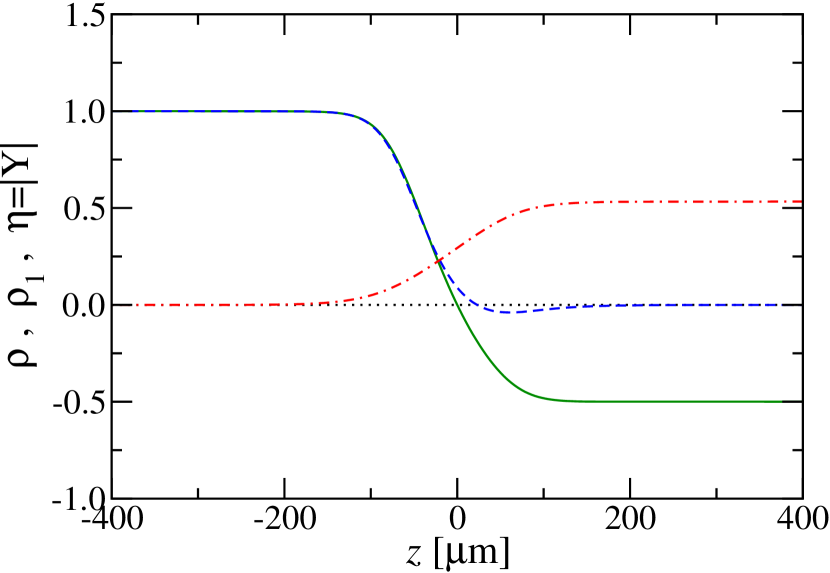
Figure 1: (Color online) The dimensionless renormalized temperature parameters $\rho$ (green solid line), $\rho_{1}$ (blue dashed line), and the modulus of the order parameter $\eta=|Y|$ (red dash-dotted line) for the superfluid/normal-fluid interface.

In Fig. 1 we observe three different regions. For low altitudes $z\lesssim-100\,\mathrm{\mu m}$ we find the asymptotic values $\rho\to 1$, $\rho_{1}\to 1$, and $\eta=|Y|\to 0$. Hence, in this region the ⁴He is normal fluid. We recover the related flow parameter condition $\rho=1$ of Ref. Do85, in the asymptotic limit $z\to-\infty$. For high altitudes $z\gtrsim+100\,\mathrm{\mu m}$ we find the asymptotic values $\rho\to-1/2$, $\rho_{1}\to 0$, and $\eta=|Y|\to(A_{d}/8u)^{1/2}$ where $A_{d}=1/4\pi$ for $d=3$. Hence, in this latter region the order parameter is nonzero and the ⁴He is superfluid. Again, we recover the related flow parameter condition $\rho=-1/2$ of Ref. Do85, in the asymptotic limit $z\to+\infty$. The third region is the interface region $-100\,\mathrm{\mu m}\lesssim z\lesssim+100\,\mathrm{\mu m}$. Here the curves interpolate between the asymptotic values. We clearly see that the interface induced by gravity has a thickness of about $\Delta z_{I,g}\approx 200\,\mathrm{\mu m}$.

Since the system is constant with respect to the horizontal coordinates $x$, $y$, and with respect to the time $t$, the covariant derivatives of the dimensionless renormalized quantities are nonzero only for the altitude coordinate $z$. In most cases these covariant derivatives are calculated by numerical differentiation using the formulas derived in section III.5. An exception is $\xi D_{z}\rho_{1}$ which is expressed in terms of other covariant derivatives by formula (97). The result is shown in Fig. 2 by the blue dashed line. Alternatively, we apply Eq. (96) to the modified temperature parameter $\rho_{1}$ and calculate the covariant derivative directly by numerical differentiation. This latter procedure is not correct in the interface region where the renormalization factors depend on the altitude coordinate because $\rho_{1}$ is not renormalized as $\rho$. Nevertheless, in Fig. 2 the result is shown by the blue solid line. Surprisingly, the two blue lines, the solid one and the dashed one, are close to each other. Hence, Eq. (96) is not that bad for calculating the covariant derivative $\xi D_{z}\rho_{1}$.

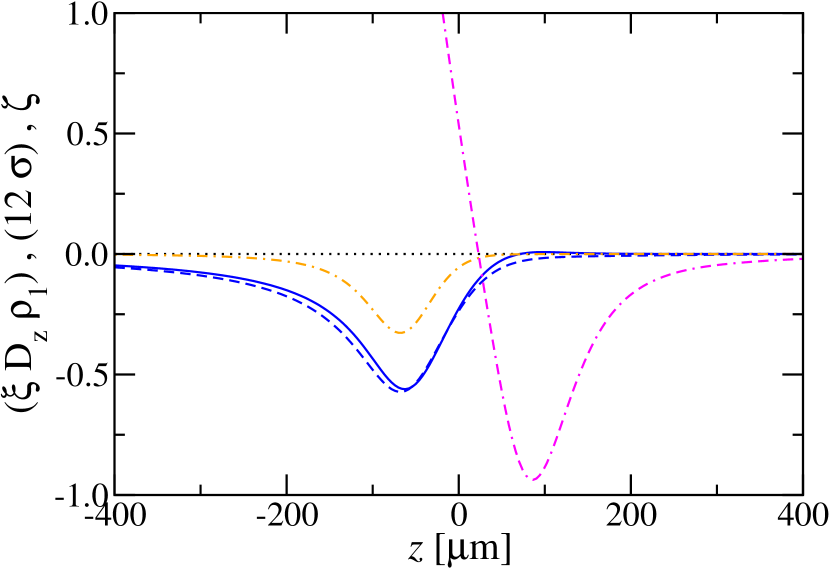
Figure 2: (Color online) The blue lines show the dimensionless covariant derivative $\xi D_{z}\rho_{1}$ calculated in two ways: by numerical differentiation (blue solid line) and by formula (97) (blue dashed line). Furthermore the parameter $\sigma$ defined in (114) and multiplied by a factor $12$ is shown as orange dash-dotted line. Finally, the argument of the function (79) $\bar{\zeta}$ is shown as magenta double-dash-dotted line.

The blue lines in Fig. 2 represent the covariant derivative of the blue dashed line in Fig. 1. However, the latter line represents $\rho_{1}=\rho_{1}(z)$ and shows a negative minimum value $\rho_{1,\mathrm{min}}<0$ at the position $z_{\mathrm{min}}\approx 60\,\mathrm{\mu m}$. Consequently for $\xi D_{z}\rho_{1}$ we expect a zero at this position related to a sign change. In Fig. 2 the solid blue line does show this zero and sign change but the dashed blue line does not. In this way, the apparently incorrect formula (96) for $\rho_{1}$ appears to be more realistic than the generic formula (97).

The existence of the sign change is supported by the following argument. In a small $z$ interval close to the interface we may modify the renormalization-group theory by choosing a constant flow parameter $\tau$. In this case the covariant derivatives reduce to the partial derivatives so that Eqs. (96) and (97) would yield identical results for $\xi D_{z}\rho_{1}=\xi\partial_{z}\rho_{1}$ and the two blue lines in Fig. 2 would collapse to a single line. As a result the sign change would be found at $z_{\mathrm{min}}$ if we evaluate the partial derivative explicitly by differentiation of the blue dashed line in Fig. 1.

However, the sign change of the solid blue line in Fig. 2 would have a dramatic consequence for the numerical procedure when calculating $\sigma$ and the amplitudes $A$ and $A_{1}$. In thermal equilibrium we have $\Delta\rho=0$ so that Eq. (114) reduces to $\sigma=-(\xi D_{z}\rho_{1})^{2}/12$. Consequently, $\sigma$ will be negative everywhere except at a point close to $z_{\mathrm{min}}$. At this point we have $\sigma=0$ so that the formulas for the amplitudes $A$ and $A_{1}$ reduce to (69) and (70), respectively. However, close to the minimum position $z_{\mathrm{min}}$ the modified temperature parameter $\rho_{1}$ is negative which implies an imaginary result for $\rho_{1}^{-\varepsilon/2}$ in Eqs. (69) and (70) where $\varepsilon=4-d=1$ for $d=3$. Hence, the amplitudes $A$ and $A_{1}$ are not well defined if the solid line in Fig. 2 and the formula (96) is used.

The problem arises due to the fact that we evaluate the Green function (23), the condensate density $n_{\mathrm{s}}$, the superfluid current $\mathbf{J}_{\mathrm{s}}$, and hence the amplitudes $A$ and $A_{1}$ in an approximation where only the covariant gradients of the temperature parameters $\rho_{1}$ and $\Delta\rho$ are taken into account. If we could do the calculation for the full space dependence all these quantities would be well defined. In the unpublished work HN08 we extended the calculation by including also the curvatures of the temperature parameters. While the problem at $z_{\mathrm{min}}$ was abolished, the calculation was much more complicated and restricted to the thermal equilibrium at zero heat current. Moreover, other mathematical difficulties appeared. Hence, this more sophisticated calculation could not be realized in practice for our purpose.

However, our fortune is a small inaccuracy of the approximation in our numerical calculation in practice which implies that the blue dashed line in Fig. 2 is completely negative and does not show a zero and a sign change for the covariant derivative $\xi D_{z}\rho_{1}$. The related parameter $\sigma=-(\xi D_{z}\rho_{1})^{2}/12$ is shown in Fig. 2 as orange dash-dotted line where it has been enhanced by a factor $12$. Clearly, this curve is negative and never zero for all altitudes $z$ in the interface region. For this reason we can apply our formulas (80) and (81) for the amplitudes $A$ and $A_{1}$ without a problem if we use the generic formula (97) for the dimensionless gradient $\xi D_{z}\rho_{1}$. We obtain smooth and stable results which are within the accuracy of our approximation.

In order to evaluate the amplitudes $A$ and $A_{1}$ we need the function (79) and its argument $\bar{\zeta}=\rho_{1}/(-\sigma)^{1/3}$. Consequently, from the dashed blue line in Fig. 1 and the orange dash-dotted line in Fig. 2 we obtain the dimensionless variable $\bar{\zeta}$ as a function of the altitude coordinate $z$ which is shown in Fig. 2 by the magenta double-dash-dotted line. In the normal-fluid region for $z<0$ the variable $\bar{\zeta}$ increases quickly for decreasing altitude $z$. Consequently, in this case the asymptotic formula (82) can be used so that the amplitudes $A$ and $A_{1}$ reduce to the simple formulas (69) and (70) of the normal-fluid equilibrium state. In the superfluid region near the interface the variable $\bar{\zeta}$ is negative. However, it is bounded from below by the value $-1$. Consequently, the asymptotic formula (83) is not needed. This means that the variable $\bar{\zeta}$ never comes in the large negative region where the function (79) oscillates and possesses a significant imaginary part. This observation is very important for the consistency of our theory because the oscillations would be unphysical and the imaginary part would be related to an instability.

IV.2 Temperature profiles

Until now, the calculations are restricted to the thermal equilibrium at zero heat current $Q=0$. Here the phase of the order parameter $Y=\eta\,e^{i\varphi}$ is constant, so that we can chose $\varphi=0$. We have extended our numerical calculations to small nonzero heat currents $Q$ in the interval $-70\,\mathrm{nW/cm^{2}}\leq Q\leq+160\,\mathrm{nW/cm^{2}}$. In this latter case the phase of the order parameter $\varphi=\varphi(z,t)$ will be a nontrivial function of the altitude coordinate $z$ and the time $t$. A positive heat current $Q>0$ means a heat flow $\mathbf{Q}=Q\,\mathbf{e}_{z}$ in the $z$ direction which means that the heat current flows upward from bottom to top. The original experiment by Duncan et al. DAS88 and succeeding experiments investigating the superfluid/normal-fluid interface induced by a heat current $Q$ were performed in this configuration. On the other hand a negative heat current $Q<0$ means a downward heat flow from top to bottom. This latter configuration was investigated much later in the experiment by Moeur et al. Du97 .

In the nonequilibrium system with a nonzero heat flow the dimensionless renormalized temperature parameter $\Delta\rho$ will be nonzero. Once the local space and time dependent RG flow parameter $\tau=\tau(z,t)$ is known, the space and time dependent temperature profile $T=T(z,t)$ is calculated from $\Delta\rho$ by Eq. (56). Furthermore, the local space and time dependent heat current $Q=Q(z,t)$ is calculated from the dimensionless renormalized heat current $\tilde{q}$ by Eq. (124). After a time difference of about $\delta t=2\,\mathrm{s}$ the system will relax in a stationary state where all quantities are constant in time. If in Eq. (122) the source and sink parameters $Q_{1}=Q_{2}=Q$ are chosen, a vertical heat current $Q$ will be found in the whole system which is constant in the space variable $z$. Consequently, the different temperature profiles we obtain in our numerical calculations can be labeled by this constant heat current.

Our numerical results are shown in Fig. 3. The temperature profile $T(z)$ is shown by the colored solid lines for several values of the heat current $Q$ which are specified in the caption of the figure. On the other hand, the superfluid transition temperature $T_{\lambda}(z)$ as a function of the altitude coordinate $z$ is shown by the straight black dashed line. The slope of this latter line is the effect of the gravity on earth.

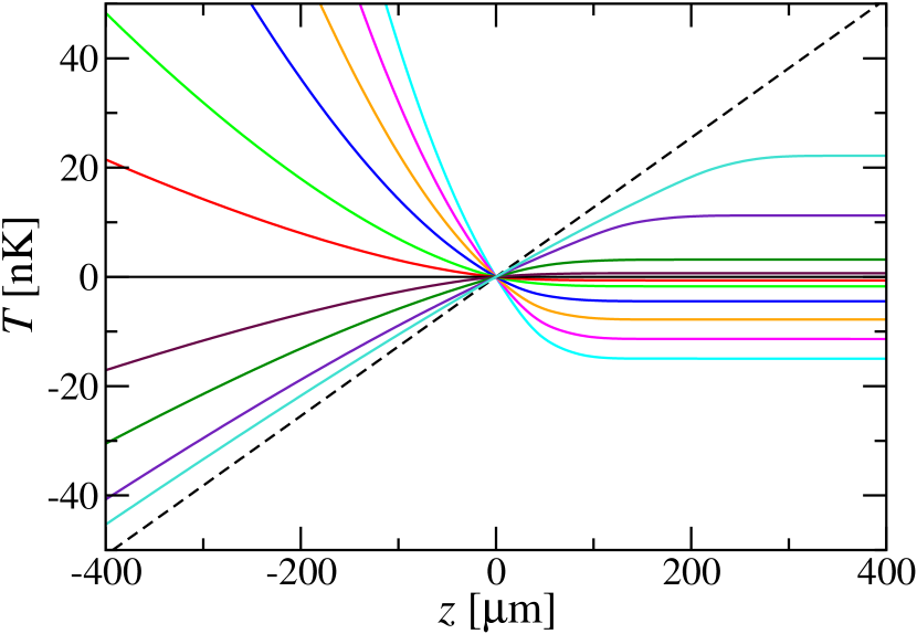
Figure 3: (Color online) The temperature profiles $T(z)$ of the superfluid/normal-fluid interface of liquid ⁴He in gravity are shown for several heat currents $Q$ as colored solid lines. The solid lines on the left-hand (normal-fluid) side are ordered from top to bottom with respect to decreasing heat currents $Q=160$, $130$, $100$, $70$, $40$, $20$, $0$, $-20$, $-40$, $-60$, $-70\,\mathrm{nW/cm^{2}}$. On the right-hand (superfluid) side they are ordered from bottom to top. The horizontal black solid line represents the temperature in thermal equilibrium for $Q=0$. The straight black dashed line represents the superfluid transition temperature $T_{\lambda}(z)$.

The altitude $z_{0}$ at which the temperature profiles $T(z)$ and $T_{\lambda}(z)$ intersect each other so that $T(z_{0})=T_{\lambda}(z_{0})$ may be viewed as a reference altitude to specify the position of the superfluid/normal-fluid interface. We realize that the system is translation invariant in the sense that we can move the curves parallel along the straight dashed line. Thus, for convenience and simplicity we select a coordinate system so that all curves intersect at the same altitude $z=z_{0}=0$. This choice is no physical restriction and has been applied in Fig. 3.

On the left hand side for low altitudes $z\lesssim-100\,\mathrm{\mu m}$ the system is normal fluid. Here the heat transport equation $Q=-\lambda_{T}\partial_{z}T$ implies that the temperature gradient $\partial_{z}T$ is negative for positive heat currents $Q$ and positive for negative heat currents. The values of the gradients are considerably large. On the right hand side for high altitudes $z\gtrsim+100\,\mathrm{\mu m}$ the system is superfluid. Here the heat is transported convectively following the two-fluid model so that the temperatures $T(z)$ are nearly constant and the gradients are nearly zero. The intermediate region $-100\,\mathrm{\mu m}\lesssim z\lesssim+100\,\mathrm{\mu m}$ is the superfluid/normal-fluid interface. Here the temperature profiles interpolate the two outer regions.

For positive heat currents $Q>0$ (heat flow upward) the slope of the temperature curve $T(z)$ increases without a limit on the normal-fluid side for $z\to-\infty$. However, for negative heat currents $Q<0$ (heat flow downward) the slope increases up to a limiting value which is the slope of $T_{\lambda}(z)$ so that in the limit $z\to-\infty$ the temperature profile $T(z)$ approaches a straight line parallel to the straight dashed line $T_{\lambda}(z)$. This latter fact is clearly observed in the lower left part of Fig. 3. It represents the self-organized critical state predicted by Onuki On87 and discovered in the experiment by Moeur et al. Du97 .

While Figs. 1 and 2 are calculated for the thermal equilibrium at zero heat current $Q=0$, we have calculated the related curves also for the nonequilibrium state at the nonzero heat currents of Fig. 3. Most curves do not change very much, the characteristic forms remain qualitatively. An exception is the parameter $\sigma$ defined in Eq. (114) and shown as orange dash-dotted line in Fig. 2. This parameter is negative in the whole system only for small heat currents in the interval $-10\,\mathrm{nW/cm^{2}}\lesssim Q\lesssim+20\,\mathrm{nW/cm^{2}}$. For larger heat currents outside this interval the parameter $\sigma$ will change the sign from negative to positive at specific altitudes $z$. For even larger negative heat currents $Q\lesssim-20\,\mathrm{nW/cm^{2}}$ and even larger positive heat currents $Q\gtrsim+40\,\mathrm{nW/cm^{2}}$ the parameter $\sigma$ is positive in the whole system.

IV.3 Order parameter

The order parameter in physical units $\langle\psi\rangle$ is calculated from the dimensionless renormalized order parameter $Y$ via the renormalization formulas (30) and (60). Putting these equations together and replacing $\mu\to\xi^{-1}$ we obtain

$$\langle\psi\rangle=Z_{\phi}^{1/2}\,Y\,\xi^{-(d-2)/2}\ .$$ (125)

Integrating the defining equation (85) for the zeta function $\zeta_{\phi}$, we obtain an integral representation for the renormalization factor

$$Z_{\phi}=\exp\Bigl{\{}\int_{\mu}^{\infty}\zeta_{\phi}\,\frac{d\mu^{\prime}}{\mu^{\prime}}\Bigr{\}}=\exp\Bigl{\{}-\int_{\tau}^{\infty}\nu\eta\,\frac{d\tau^{\prime}}{\tau^{\prime}}\Bigr{\}}\ .$$ (126)

The second equality sign is implied by the flow-parameter transformation (89) together with the running exponents $\nu$ and $\eta$, defined in (99) and (100). The upper infinite integration boundaries guarantee $Z_{\phi}=1$ in the limits $\mu\to\infty$ and $\tau\to\infty$ which represent the mean-field or Gaussian fix point of the RG flow. If we use the correlation length $\xi=\xi_{0}\,\tau^{-\nu}$ we obtain the asymptotic formula for the order parameter $\langle\psi\rangle\sim\tau^{\nu(d-2+\eta)/2}=\tau^{\beta}$ with the correct critical exponent $\beta$ defined in (101).

Eqs. (125) and (126) are suited for a numerical calculation once the dimensionless renormalized order parameter $Y$, the RG flow parameter $\tau$, and the running exponents (99)-(101) are known. We have calculated the order parameter $\langle\psi\rangle=M\,e^{i\varphi}$ in the stationary state for all those heat currents $Q$ for which we have calculated the temperature profiles in the previous subsection. We obtain the modulus $M$ and the phase $\varphi$ of the order parameter. Our results for the modulus $M$ are shown in Fig. 4 for positive heat currents $Q\geq 0$ (heat flow upward). The colors of the solid lines correspond to those in Fig. 3. Here and in the following figures we omit the lines for negative heat currents $Q<0$ (heat flow downward) because they make the figures complicated and involved but do now show new physics.

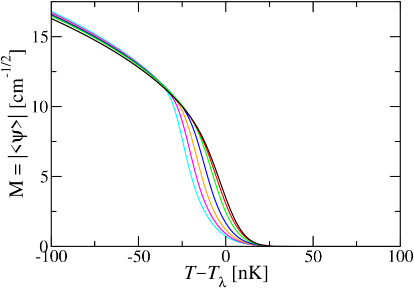
Figure 4: (Color online) The modulus of the order parameter $M=|\langle\psi\rangle|$ as a function of the temperature difference $T-T_{\lambda}$ for the superfluid/normal-fluid interface in gravity. The colored solid lines from left to right represent the heat currents $Q=160$, $130$, $100$, $70$, $40$, $20$, $0\,\mathrm{nW/cm^{2}}$.

Close to criticality $T=T_{\lambda}$ the curves are smooth. This is an effect of gravity and related to the superfluid/normal-fluid interface. The width of the smooth region is $\Delta T_{I,g}=25\,\mathrm{nK}$ which corresponds to the thickness of the interface $\Delta z_{I,g}=200\,\mathrm{\mu m}$. The ratio is approximately the gradient of the superfluid transition temperature, i.e. $\Delta T_{I,g}/\Delta z_{I,g}\approx\partial T_{\lambda}/\partial z=1.273\,\mathrm{\mu K/cm}$. For increasing heat currents $Q$ the smooth curves are shifted to the left to lower temperatures. This fact is related to the depression of the superfluid transition to lower temperatures by a heat current which has been observed and investigated in the experiment by Duncan, Ahlers, and Steinberg DAS88 .

Away from criticality for lower temperatures $T-T_{\lambda}\lesssim-30\,\mathrm{nK}$ the curves approach asymptotically a single line which corresponds to the singular order parameter $M=|\langle\psi\rangle|\sim(T_{\lambda}-T)^{\beta}$ for $T<T_{\lambda}$ in thermal equilibrium and zero gravity. In Fig. 4 the asymptotic curves do not fall perfectly on a single line. This observation is a numerical error in our calculation. In order to stabilize the numerical iterations we must add an imaginary part to the parameter $\sigma$ defined in (114). This imaginary part increases with increasing heat current $Q$ and influences slightly the curves on the superfluid side.

The physical units $\mathrm{cm}^{-1/2}$ of the order parameter arising from the formula (125) for $d=3$ dimensions appear to be artificial and unphysical. However, since the order parameter can not be observed in physical experiments, this artifact is not important and no matter of concern.

The phase of the order parameter $\varphi$ is dimensionless. Its gradient is related to the superfluid velocity $\mathbf{v}_{\mathrm{s}}=(\hbar/m_{4})\nabla\varphi$. For nonzero heat currents $Q$ we find nontrivial results for the superfluid velocity $v_{\mathrm{s}}$. If we approach the interface from the superfluid side, $v_{\mathrm{s}}$ increases monotonically. However, on the normal-fluid side, the phase $\varphi$ and the superfluid velocity $v_{\mathrm{s}}$ are irrelevant because the modulus $M$ approaches zero.

IV.4 Correlation length

The correlation length $\xi$ has been calculated by Schloms and Dohm SD89 in thermal equilibrium and zero gravity. In the renormalized perturbation theory up to two-loop order they obtain $\xi^{-2}=\mu^{2}A_{\xi}$ with an amplitude function $A_{\xi}=1+\mathcal{O}(u^{2})$. However, since our Hartree approximation is first order in $u$ we may approximate $A_{\xi}\approx 1$, so that the correlation length is just $\xi=\mu^{-1}$. This quantity is provided by our numerical calculation. Our results are shown in Fig. 5 by the colored solid lines for the same positive heat currents as in the previous figures. In the interface region close to criticality $T=T_{\lambda}$ the colored solid curves are smooth. The correlation length has a maximum value $\xi_{g}\approx 50\,\mathrm{\mu m}$ which is implied by the gravity acceleration $g=9.81\,\mathrm{m/s^{2}}$ on earth. The effect of a small nonzero heat current $Q$ is weak. For increasing heat currents $Q$ the position of the maximum of the correlation length is shifted slightly to lower temperatures. We note that our maximum correlation length $\xi_{g}$ is of the same order of magnitude as the characteristic length $l_{g}=67\,\mathrm{\mu m}$ which was used by Ginzburg and Sobyanin GS76 within their $\psi$ theory.

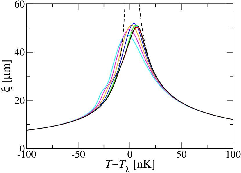
Figure 5: (Color online) The correlation length $\xi$ as a function of the temperature difference $T-T_{\lambda}$ for the superfluid/normal-fluid interface in gravity. The colored solid lines from left to right represent the heat currents $Q=160$, $130$, $100$, $70$, $40$, $20$, $0\,\mathrm{nW/cm^{2}}$. As a reference the black dashed line shows the singular correlation length in thermal equilibrium and zero gravity.

From Fig. 1 we have inferred the interface thickness $\Delta z_{I,g}=200\,\mathrm{\mu m}$. Thus we calculate the ratio $\Delta z_{I,g}/\xi_{g}\approx 4$ which means that the interface thickness is four times the maximum of the correlation length. While in a nonequilibrium and/or gravity environment the correlation length $\xi$ is finite and a smooth function, in equilibrium and zero gravity it shows the well known singular behavior $\xi\sim|T-T_{\lambda}|^{-\nu}$ near criticality for $T\to T_{\lambda}$ with an exponent $\nu=0.671$. This latter singular correlation length is shown by the black dashed line which diverges at $T=T_{\lambda}$. Far away from criticality which means far away from the interface all solid lines converge to a single line which is identical with the black dashed line. Thus, far away from the interface the gravity $g$ and the heat current $Q$ do not have an influence on the correlation length $\xi$. Finally, here we do not see an influence of the imaginary part of the parameter $\sigma$ we introduce in our calculation in order to stabilize the numerical iterations.

IV.5 Specific heat

There are two possibilities to calculate the specific heat. First, we may calculate the entropy $S$ within our renormalization-group theory and then calculate the derivative $C_{X}=T(\partial S/\partial T)_{X}$ numerically where any quantity $X$ may be kept constant. This has been done in our previous paper Ha99a where $X=Q$ or $X=\nabla T$. The entropy $S$ is given by Eqs. (8.10) or (8.12) of Ref. Ha99a, . Secondly, we calculate the specific heat directly by $C=k_{\mathrm{B}}\chi_{0}Z_{m}C_{\mathrm{ren}}$ where the renormalized specific heat $C_{\mathrm{ren}}$ is defined in (51) and the renormalization factor $\chi_{0}Z_{m}$ is defined implicitly in (59). Thus, we obtain

$$C_{X}=k_{\mathrm{B}}\frac{A_{d}}{4\tau^{2}\xi^{d}}\,\Bigl{\{}\frac{1}{\gamma^{2}}+\frac{1}{2u}\Bigl{[}1-\Bigl{(}\frac{\partial\rho_{1}}{\partial\rho}\Bigr{)}_{X}\Bigr{]}\Bigr{\}}\ ,$$ (127)

a formula which should be compared with the entropy (8.10) in Ref. Ha99a, . The formula can be simplified if we use the asymptotic formulas for the correlation length $\xi=\xi_{0}\,\tau^{-\nu}$ and for the coupling parameter $\gamma^{-2}=(4\nu/\alpha)(1-b\tau^{\alpha})$ where $\nu=0.671$ and $\alpha=2-d\nu=-0.013$ are critical exponents and $b$ is a known constant. As a result we obtain the specific heat

$$C_{X}=B+\tilde{A}\{(4\nu/\alpha)+F_{X}[u]\}\tau^{-\alpha}$$ (128)

together with the amplitude

$$F_{X}[u]=\frac{1}{2u}\Bigl{[}1-\Bigl{(}\frac{\partial\rho_{1}}{\partial\rho}\Bigr{)}_{X}\Bigr{]}\ .$$ (129)

This formula should be compared with the entropy (8.12) in our previous paper Ha99a together with Eqs. (8.13)-(8.16). Here $\tilde{A}$ and $B$ are nonuniversal constants which can be expressed in the forms $\tilde{A}=k_{\mathrm{B}}A_{d}/4\xi_{0}^{d}$ and $B=\tilde{A}(-4\nu/\alpha)b$. Alternatively, these constants can be obtained by fitting the formula to the experimental data for liquid ⁴He in a micro gravity environment in space Li96 ; Li03 . In this way we obtain $\tilde{A}=2.22\,\mathrm{J/mol\,K}$ and $B=456\,\mathrm{J/mol\,K}$ where the constants are multiplied additionally by the molar volume of liquid ⁴He at saturated vapor pressure Al85 $V_{\lambda}=27.38\,\mathrm{cm^{3}/mol}$.

The amplitude $F_{X}[u]$ can be compared directly with the amplitudes $F_{\pm}[u]$ of Dohm Do85 , if we consider the asymptotic limits far away from the interface. The temperature parameters $\rho$ and $\rho_{1}$ are related to each other by (65). In the normal-fluid region far away from the interface the renormalized order parameter is $Y=0$ and the amplitudes $A$ and $A_{1}$ are given by (69) and (70). The partial derivative can be performed easily so that we obtain $\partial\rho/\partial\rho_{1}=1+8u\,A_{1}=1-4u$ which does not depend on the variable $X$ that is kept constant. Thus we obtain the amplitude

$$F_{+}[u]=(2u)^{-1}[1-1/(1-4u)]=-2+\mathcal{O}(u)\ .$$ (130)

In the superfluid region $\rho_{1}$ approaches $0$ more rapidly than $\rho$ approaches $-1/2$. Consequently, in the superfluid region far away from the interface the partial derivative is $\partial\rho_{1}/\partial\rho=0$ which again does not depend on the variable $X$ that is kept constant. Thus we obtain the amplitude $F_{-}[u]=(2u)^{-1}$. If we compare our results for $F_{\pm}[u]$ with those of Dohm Do85 we find agreement for the leading terms in powers of $u$ in both cases $+$ and $-$, respectively.

We have calculated the specific heat numerically with both methods described above using the entropy formula (8.12) of our previous paper Ha99a and the specific-heat formula (128) of the present paper. The results agree with each other within the accuracy of our Hartree approximation which is a self-consistent one-loop approximation combined with the renormalization-group theory. This agreement is a test for the validity and the accuracy of our method presented in this paper. While in the previous paper we have used the first method, in this paper we prefer the second method, i.e. formula (128) together with (129). The reason is that in the present calculation the second method provides curves looking smoother and more nice.

Our results are shown in Fig. 6 by the colored solid lines for the same heat currents as in the previous figures. We have calculated the specific heat $C_{Q}$ where the heat current $Q$ and the gravity acceleration $g=9.81\,\mathrm{cm/s^{2}}$ are kept constant. Clearly, in the interface region near criticality we find smooth curves. The specific heat has a maximum slightly below the critical temperature. For increasing heat currents $Q$ this maximum is shifted to lower temperatures which is related to the depression of the superfluid transition temperature observed in the experiment by Duncan, Ahlers, and Steinberg DAS88 . Furthermore, the maximum of the specific heat is strongly enhanced for increasing heat currents $Q$. This enhancement is an effect of the constant heat current $Q$ when calculating the specific heat $C_{Q}$. It has been observed already in our previous paper Ha99a , where $C_{Q}$ has be calculated for the much higher heat current $Q=42.9\,\mathrm{\mu W/cm^{2}}$ where gravity effects are negligible. The strong enhancement of the maximum is also compatible with experimental measurements of $C_{Q}$ by Harter et al. HL00 .

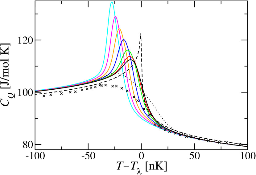
Figure 6: (Color online) The specific heat $C_{Q}$ as a function of the temperature difference $T-T_{\lambda}$ for the superfluid/normal-fluid interface in gravity. The colored solid lines from left to right represent the heat currents $Q=160$, $130$, $100$, $70$, $40$, $20$, $0\,\mathrm{nW/cm^{2}}$. The black dashed line represents the singular specific heat in microgravity fitted to the data of the experiment by Lipa et al. Li96 ; Li03 . The black crosses show the experimental data for zero heat current in gravity on earth by Lipa Li11 where the black dotted line is the related theoretical curve for the average specific heat $\bar{C}_{Q}$.

Far away from criticality and the interface on both sides the colored solid curves converge to a single line, respectively. These single lines represent the asymptotic specific heat $C=B+(A_{\pm}/\alpha)|t|^{-\alpha}$ where $t=(T-T_{\lambda})/T_{\lambda}$ is the reduced temperature and $\alpha$ is the critical exponent. On the normal-fluid side the single line is perfect. However, on the superfluid side it is slightly influenced by the imaginary part of the parameter $\sigma$ which we must add in our numerical calculation in order to have stable iterations. This fact is related to the similar observation in our results for the order parameter shown in Fig. 4.

The smooth colored solid lines in Fig. 6 show that the critical singularity is rounded by the gravity $g$ and the heat current $Q$. The temperature scale for this rounding is $\Delta T_{g,I}=25\,\mathrm{nK}$ if gravity is the dominating effect. We have obtained this value from the thickness of the interface $\Delta z_{I,g}=200\,\mathrm{\mu m}$. Consequently, the asymptotic critical behavior of the specific heat and all other singular quantities can be observed only for temperatures $|T-T_{\lambda}|\gtrsim\Delta T_{g,I}=25\,\mathrm{nK}$ away from criticality. Hence, the gravity implies that on earth the critical point can never be reached. For this reason, experiments to measure the asymptotic behavior closer to the critical point must be performed in a micro-gravity environment in space.

Lipa et al. Li96 ; Li03 have performed a space experiment which was called Lambda Point Experiment (LPE) and which flew aboard the space shuttle Columbia (STS-52) in 1992. They obtained data for the specific heat up to $|T-T_{\lambda}|=1\,\mathrm{nK}$. They fitted an asymptotic formula to the data and determined the exponent $\alpha=-0.013$, the amplitudes $A_{\pm}$ and $B$ and some further parameters. The resulting fit curve is shown in Fig. 6 by the black dashed line. This curve shows the typical lambda of the specific heat with a singularity at $T=T_{\lambda}$. Away from criticality on both sides for $|T-T_{\lambda}|\gtrsim 50\,\mathrm{nK}$ the solid lines and the dashed line come close to each other which demonstrates the agreement between theory and experiment. However, the agreement is not perfect. There remains a small discrepancy which is due to the amplitude ratio $A_{+}/A_{-}$ because our theory provides an approximate value for this amplitude ratio which can never be identical to the experimental value.

We note that in our calculation the specific heat is defined locally. It depends on the altitude $z$ so that $C_{Q}=C_{Q}(z)$. The rounding of the critical singularity is caused by the gradient of $T_{\lambda}(z)$ and by the heat current only. However, in experiments the ⁴He is in a cell of a finite extension. The cell is usually confined by two horizontal plates at altitudes $z_{1}$ and $z_{2}$, where the vertical height $L=z_{2}-z_{1}$ is small and the horizontal extensions are large. For this reason the experiment measures an average specific heat which is defined by the integral $\bar{C}_{Q}=(z_{2}-z_{1})^{-1}\int_{z_{1}}^{z_{2}}dz\,C_{Q}(z)$. This average process smooths the curve additionally. The maximum of the average specific heat $\bar{C}_{Q}$ will be broader than the maximum of the related local specific heat $C_{Q}$.

In order to minimize the averaging effects the cell height $L$ should be chosen as small as possible. However, it must be considerably larger than the maximum correlation length $\xi_{g}=50\,\mu m$ because for small $L$ finite size effects occur which again smooth and round the critical singularity. Consequently, for the cell height $L$ there will be an optimum range to obtain best measurements on earth.

In Fig. 6 the black crosses represent the experimental data of a measurement on earth at zero heat current performed by Lipa Li11 . In this case the cell height is $L=0.38\,mm$ which causes considerable average effects. The maximum of the experimental data is much broader than the maximum of the black solid line which represents the local specific heat $C_{Q}$ for $Q=0$. We have calculated the related average specific heat $\bar{C}_{Q}$ for $Q=0$ which is shown by the black dotted line. This latter curve shows a much broader maximum at criticality which agrees with the experimental data. Since the ratio $L/\xi_{g}=7.6$ is large, finite size effects are small. However, the Dirichlet boundary conditions of the order parameter at the cell walls imply that nevertheless the finite size effects cause a depression of the data which is clearly observed in Fig. 6 because the experimental data (black crosses) are below the theoretical curve (black dotted line). Thus we conclude that the experimental data obtained in a measurement in gravity on earth agree with our theory.

IV.6 Thermal conductivity and resistivity

The thermal conductivity $\lambda_{\mathrm{T}}$ is defined locally by the heat transport equation $\mathbf{Q}=-\lambda_{\mathrm{T}}\nabla T$. Resolving this equation we obtain the thermal conductivity explicitly as $\lambda_{\mathrm{T}}=|\mathbf{Q}|/|\nabla T|$. Next we insert the renormalization equations for the heat current (124) and for the temperature gradient (94). Thus, we obtain

$$\lambda_{\mathrm{T}}=\frac{g_{0}k_{\mathrm{B}}}{\tau\,\xi^{d-2}}\,\frac{|\tilde{\mathbf{q}}|}{|\xi\mathbf{D}\Delta\rho|}\ .$$ (131)

The dimensionless heat current $\tilde{\mathbf{q}}$ and the dimensionless renormalized gradient $\xi\mathbf{D}\Delta\rho$ are variables in our numerical calculation. Hence Eq. (131) is well suited for an explicit calculation of the thermal conductivity.

The dimensionless renormalized heat current is defined in (111). Far away from the interface in the normal-fluid region the order parameter $Y$ and hence the last term of (111) is zero. On the other hand, the amplitude $A_{1}$ in the first term of (111) reduces to $A_{1}=-1/2$ following (70). Thus Eq. (131) provides the thermal conductivity

$$\lambda_{\mathrm{T}}=\frac{g_{0}k_{\mathrm{B}}}{\tau\,\xi^{d-2}}\,\frac{A_{d}}{2\gamma F}\,\Bigl{\{}1-\frac{f}{4}\Bigr{\}}\ .$$ (132)

in the normal-fluid region. This result is well known and agrees with the linear-response calculation of Dohm Do85 . Since our result is derived in Hartree approximation, the agreement is up to one-loop order.

Far away from the interface in the superfluid region the heat current $\mathbf{Q}$ is nonzero where the temperature gradient $\nabla T$ is zero. Hence the thermal conductivity $\lambda_{\mathrm{T}}$ is infinite. This fact is also seen in the formulas (111) and (131). A zero dimensionless renormalized temperature gradient $\xi\mathbf{D}\Delta\rho=\mathbf{0}$ implies a zero first term in (111) and a zero denominator in (131). On the other hand, the second term in (111) is minus the dimensionless renormalized superfluid current which is nonzero. Consequently, Eq. (131) provides an infinite thermal conductivity once again in the superfluid region.

A related quantity is the thermal resistivity $\rho_{\mathrm{T}}=1/\lambda_{\mathrm{T}}$ which is the inverse of the thermal conductivity. In the normal-fluid region the thermal resistivity $\rho_{\mathrm{T}}$ is finite. On the other hand, in the superfluid region it is zero. For this reason the thermal resistivity $\rho_{\mathrm{T}}$ is well suited for a graphical representation. In Fig. 7 the results of our numerical calculation are shown as colored solid lines for several positive values of the heat current $Q$. These heat currents are the same as those in the previous figures. Clearly, in the interface region near criticality the colored solid curves are smooth lines. The critical singularity at $T=T_{\lambda}$ is smoothed by the nonzero values of gravity $g$ and the heat current $Q$. For increasing heat currents $Q$ the colored solid lines are shifted to lower temperatures. This fact is again related to the depression of the superfluid transition temperature by nonzero heat currents following Duncan, Ahlers, and Steinberg DAS88 .

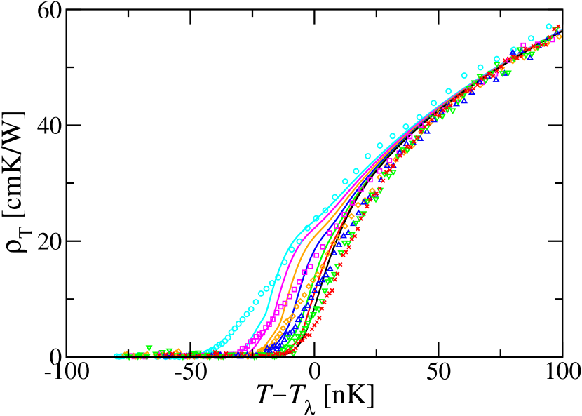
Figure 7: (Color online) The thermal resistivity as a function of the temperature difference $T-T_{\lambda}$ for the superfluid/normal-fluid interface in gravity. The colored solid lines from left to right represent the heat currents $Q=160$, $130$, $100$, $70$, $40$, $20$, $0\,\mathrm{nW/cm^{2}}$. The data points represent the experimental data by Day et al. Du98 taken for the same heat currents except $Q=0$. Related to the theoretical curves the data are ordered from left to right.

On both sides far away from criticality $T=T_{\lambda}$ and from the interface the colored curves asymptotically approach single lines, respectively. In the normal-fluid region the asymptotic thermal resistivity is given by (132), where in the superfluid region it is just zero.

The local thermal resistivity $\rho_{\mathrm{T}}$ has been measured for the superfluid/normal-fluid interface in the experiment by Day et al. Du98 . While gravity on earth is $g=9.81\,\mathrm{m/s^{2}}$, the heat current is flowing upward from bottom to top so that $Q$ is positive. The values of heat current $Q$ are the same as in our calculation. For this reason, our colored solid lines can be compared directly with the experimental data. In Fig. 7 the experimental data for several heat currents $Q$ are represented by points of several symbol types. The data points can be related to the solid curves by their color or alternatively by there order from left to right. An exception is the black solid line for zero heat current $Q=0$. In this latter case no experimental data are available. However, the black solid line is very close to the red solid line for $Q=20\,\mathrm{nW/cm^{2}}$. Consequently for $Q\lesssim 20\,\mathrm{nW/cm^{2}}$ the effect of the heat current is very small.

Qualitatively, the experimental data agree with the theoretical solid lines. However, there are quantitative discrepancies. First of all, in the normal-fluid region well above criticality for temperature differences $T-T_{\lambda}\gtrsim 50\,\mathrm{nK}$ the thermal resistivity converges to a single line represented by the formula (132). We have multiplied the theoretical results with a correction factor which slightly differs from unity. In this way we achieve that far away from criticality the experimental data are lying on top of the theoretical curves. This correction factor is justified, because in Ref. Do85, the model-$F$ parameters were adjusted for the theoretical specific heat and thermal resistivity in two-loop order where in the present paper and also in our previous papers Ha99 ; Ha99a the quantities were calculated in the Hartree approximation which is a self-consistent one-loop approximation.

For larger heat currents $Q$ and temperatures $T$ slightly below $T_{\lambda}$ our solid lines show some bumps which are probably artifacts of our approximation. The magnitude of the artifacts is within the accuracy of our approach. In the superfluid region well below criticality for temperature differences $T-T_{\lambda}\lesssim-50\,\mathrm{nK}$ the thermal resistivity $\rho_{\mathrm{T}}$ is very close to zero both in theory and experiment. This fact represents the frictionless heat transport by the superfluid/normal-fluid counterflow in superfluid ⁴He. Vortices are not present in our calculation presented here.

IV.7 Second sound and time dependent phenomena

Until now we have considered only stationary nonequilibrium states where a constant heat current $\mathbf{Q}=Q\,\mathbf{e}_{z}$ is flowing vertically in the ⁴He and where all time-dependent phenomena are relaxed. However, our numerical calculation solves the time-dependent model-$F$ equations so that time-dependent phenomena can be treated explicitly. In this case the order parameter $\langle\psi(z,t)\rangle$, the temperature $T(z,t)$, and the heat current density $\mathbf{Q}(z,t)=Q(z,t)\,\mathbf{e}_{z}$ are functions of altitude $z$ and time $t$. In superfluid ⁴He the most important dynamic phenomenon is second sound. We can generate a second sound pulse on the upper cell boundary $z_{2}$ if in the external heat source (122) we choose a time-dependent upper source function $Q_{2}(t)$. Then the phase of the order parameter $\varphi(z,t)$, the temperature $T(z,t)$, and the local heat current $Q(z,t)$ show a pulse which is traveling downward toward the superfluid/normal-fluid interface. Approaching gradually the interface the width of the pulse increases. Once the interface is reached the pulse disappears by broadening where nearly nothing is reflected. In the end the second-sound pulse is absorbed nearly completely by the interface.

A heat pulse can be generated also on the lower cell boundary $z_{1}$ if the lower source function $Q_{1}(t)$ is chosen time dependent. However, in this case the response of the system is less spectacular because on the normal-fluid side the heat is transported diffusively. Nevertheless, our time-dependent investigations yield an important result. All time-dependent perturbations of the stationary states with a constant heat flow relax and disappear. Thus we conclude that the superfluid/normal-fluid interface in gravity and in the presence of a vertical heat flow is a stable physical configuration.

V Comparison with our previous approach for large heat currents

V.1 Solutions

We have found two different solutions of the model-$F$ equations for superfluid ⁴He in the nonequilibrium state where a heat current is flowing. In the first case the order parameter $\langle\psi\rangle=M\,e^{i\varphi}$ is nonzero and no vortices are present. The heat is transported convectively without any friction by the superfluid/normal-fluid counterflow so that the temperature gradient is zero. This solution is investigated in the present paper. In the second case the order parameter is zero due to fluctuations of the phase $\varphi$ by moving vortices and quantum turbulence. Here the moving vortices imply a small thermal resistivity which causes a small temperature gradient. This latter solution was investigated in our previous papers Ha99 ; Ha99a . The two different solutions exist only in the superfluid and interface region where a nonzero order parameter is possible. In the normal-fluid region the solution is unique because here the order parameter is always zero.

The two solutions are controlled by the parameter $\sigma$ defined in Eq. (114). The first solution exists for negative and positive values of $\sigma$ where the second solution exists only for positive $\sigma$. For the superfluid/normal-fluid interface in gravity on earth this means that the first solution exist for small and large heat currents. On the other hand the second solution exists only for large heat currents $|Q|\gtrsim 70\,\mathrm{nW/cm^{2}}$ where the heat current is the major and gravity is the minor influence. However, the numerical calculations of our present paper show that in practice the first solution is stable only for small heat currents in the interval $-70\,\mathrm{nW/cm^{2}}\lesssim Q\lesssim+160\,\mathrm{nW/cm^{2}}$. For larger heat currents outside the interval we do not obtain a stable solution. We do not know if this instability is a property of our iteration procedure only which we describe in Subsec. III.6. However we guess that there is a physical instability beyond a certain critical heat current. This means we expect a discontinuous first-order like transition in the nonequilibrium state near the heat current $Q_{0}\approx 70\,\mathrm{nW/cm^{2}}$ which separates the gravity dominated regime (first solution) from the heat current dominated regime (second solution). Nevertheless, there will be an overlap region where both solutions exist.

V.2 Stability

The time-dependent nature of our numerical calculation provides a test for the physical stability of our stationary solutions. We may add a small perturbation to the solution and then start the calculation. After a time difference $\delta t\approx 2\,\mathrm{s}$ the perturbations relax and disappear so that the system returns to the stationary state. We find this behavior for all stationary solutions with a constant heat flow which we have presented in this paper. Thus, we conclude that the first-type solutions are stable which describe physical states with a nonzero order parameter and no vortices. This result is expected because the order-parameter variation and second sound are damped. We note that we have a numerical instability for larger heat currents. However, this latter instability is unphysical and has a completely different nature because it appears on the short length scales $\Delta z$ of the discretization of the altitude coordinate.

In our previous papers Ha99 ; Ha99a we did not prove the stability of the second-type solutions which describe superfluid states with vortices and a zero average order parameter. The reason is that in our previous papers we did not solve the model-$F$ equations as partial differential equations. Consequently, we do this now and provide the proof in the following. However, we note that in this case the stability is nontrivial because the system is in a superfluid state where the average order parameter is $\langle\psi\rangle=0$ and the temperature is $T<T_{\lambda}$. We solve the time-dependent renormalized model-$F$ equations for a second-type solution with a small perturbation. For simplicity we consider a self-organized critical state with a constant heat $Q$ current and constant temperature gradients $\nabla T=\nabla T_{\lambda}$ because this state is spatially homogeneous before the perturbation is applied. Unfortunately, the state is not periodic because we cannot require periodic boundary conditions for all quantities. Exceptions are the temperatures $T(z.t)$, $T_{\lambda}(z)$ and the phase of the order parameter $\varphi(z,t)$. Nevertheless, we can generalize the boundary conditions. For the latter three quantities we require pseudoperiodic boundary conditions in the sense of the impossible objects of the famous Dutch graphic artist M.C. Escher Ho79 , i.e.

$$T(z+L,t) = T(z,t)+\Delta T_{L}\ ,$$ (133)

$$T_{\lambda}(z+L) = T_{\lambda}(z)+\Delta T_{L}\ ,$$ (134)

$$\varphi(z+L,t) = \varphi(z,t)+\Delta\varphi_{L}(t)\ .$$ (135)

Since the critical temperature $T_{\lambda}(z)$ is linear in $z$, from Eq. (134) we obtain $\Delta T_{L}=(\partial_{z}T_{\lambda})L$. On the other hand from Eq. (133) we obtain $\Delta T_{L}=-(Q/\lambda_{\mathrm{T}})L$ where $\lambda_{\mathrm{T}}$ is the thermal conductivity. We note that for the self-organized critical state both results for the period constant $\Delta T_{L}$ must be equal. This fact implies $Q=-\lambda_{\mathrm{T}}(\partial_{z}T_{\lambda})$. The period constant of the order-parameter phase $\Delta\varphi_{L}(t)$ can be determined by investigating the renormalized model-$F$ equation (108). On the right-hand side we replace $\Delta\rho(z,t)$ in favor of the temperature $T(z,t)$ by inserting (56). We insert the complex order parameter $Y=\eta\,e^{i\varphi}$ and derive an equation for the order parameter phase $\varphi(z,t)$. We consider this equation for the altitudes $z=z_{0}$ and $z=z_{0}+L$ and then subtract the resulting equations. Thus, as a result we obtain $\partial_{t}\Delta\varphi_{L}(t)=g_{0}(\Delta T_{L}/T_{\lambda})$. We integrate this equation and obtain the period constant

$$\Delta\varphi_{L}(t)=\Delta\varphi_{L}(t_{0})+g_{0}(\Delta T_{L}/T_{\lambda})(t-t_{0})\ .$$ (136)

Clearly, the period of the order-parameter phase depends linearly on the time $t$. We conclude and find that for the self-organized critical state with small perturbations the renormalized model-$F$ equations can be solved numerically using Escher pseudoperiodic boundary conditions which are defined by Eqs. (133)-(135). Our numerical test provides the following result. Any small perturbation of the self-organized critical state relaxes and disappears after a time difference of $\delta t\approx 2\,\mathrm{s}$. Thus we conclude that the second-type solutions are stable. This means that the nonequilibrium states considered in the previous paper are stable.

A matter of special interest is the relaxation of the order parameter. We start at time $t_{0}$ with a small constant perturbation $Y(z,t_{0})=\eta_{0}\,e^{i\varphi_{0}}$. This means $\eta_{0}$ is small but nonzero, and $\varphi_{0}$ is constant. We consider the renormalized model-$F$ equation (108) which describes the time evolution of the order parameter $Y(z,t)=\eta(z,t)\,e^{i\varphi(z,t)}$. Decomposing the equation with respect to the modulus $\eta(z,t)$ and the phase $\varphi(z,t)$ from the first term on the right hand side we infer the damping for the modulus

$$D=g_{0}(2\gamma\,\tau)(w^{\prime}/F)[\rho_{1}+(\xi\nabla\varphi)^{2}]\ .$$ (137)

This damping is an inverse relaxation time. The solution of the model-$F$ equation is stable whenever this damping is positive and unstable otherwise. The prefactors are always positive so that the crucial quantity is the expression in the square brackets. For times $t$ shortly after the beginning of the calculation $t_{0}$ the phase is expected to be $\varphi(z,t)\approx\varphi_{0}$ so that $\nabla\varphi\approx\mathbf{0}$. Consequently, the main contribution is the dimensionless modified temperature parameter $\rho_{1}$. The stability of the solution depends on its sign. In Fig. 1 $\rho_{1}$ is plotted as the blue dashed line for the superfluid/normal-fluid interface. A similar curve is obtained for the self-organized critical state if $\rho_{1}$ is plotted as a function of the heat current $Q$. While in the normal-fluid region $\rho_{1}$ is positive, in the superfluid region it is negative. For the heat current $Q=170\,\mathrm{nW/cm^{2}}$ we find the minimum value $\rho_{1,\mathrm{min}}=-0.39$. Thus, we conclude that the solution is stable in the normal-fluid region but unstable in the superfluid region.

However, the instability is true only for short times where $t-t_{0}$ is small. For longer times we must investigate the space and time dependence of the order-parameter phase $\varphi(z,t)$. From Eq. (136) and from the renormalized model-$F$ equation (108) we infer

$$\varphi(z,t) = \varphi_{0}+\Delta\varphi_{L}(t)\,(z-z_{0})/L$$ (138)

$$= \varphi_{0}+g_{0}\,(\Delta T_{L}/T_{\lambda})\,(t-t_{0})\,(z-z_{0})/L\ .\qquad$$

Here $z_{0}$ is the altitude where the temperature equals the reference temperature, i.e. $T(z_{0},t_{0})=T_{0}$. For the last equality sign we have used (136) realizing that in our case at the beginning $t=t_{0}$ the Escher period constant is $\Delta\varphi_{L}(t_{0})=0$. Differentiating with respect to the altitude coordinate $z$ and multiplying by $\xi$ we obtain the dimensionless gradient of the order-parameter phase

$$\xi\nabla\varphi=g_{0}\,(\Delta T_{L}/T_{\lambda})\,(t-t_{0})\,(\xi/L)\,\mathbf{e}_{z}\ .$$ (139)

Consequently, we find $(\xi\nabla\varphi)^{2}\sim(t-t_{0})^{2}$. This means that in Eq. (137) the second term in the square bracket increases with time. Even though at the beginning the square bracket may be negative because of the first term, after a short time the second term makes the square bracket positive. Thus we conclude: Even though there may be an instability for short times, the increase of the gradient of the phase (139) makes the damping (137) finally positive so that the time evolution of the order parameter is finally stable.

The stability of the second model-$F$ equation (109) is easily proven. We insert the dimensionless renormalized heat current (111) and neglect its last term because it is squared in the small nonzero order parameter. As a result we obtain a diffusion equation for the dimensionless renormalized temperature parameter $\Delta\rho(z,t)$. Since the related diffusion constant is positive, this equation is always stable. The covariant derivatives in this equation do not affect the stability.

We summarize that we have presented an explicit proof for the stability of the self-organized critical state which is a spatially homogeneous second-type solution of the model-$F$ equations. We expect that also the more general second-type solutions for spatially inhomogeneous systems are stable, which describe the superfluid/normal-fluid interface in our previous papers Ha99 ; Ha99a . Our numerical calculations of the present paper support this expectation. However, we note that the stability is nontrivial because the system is in a superfluid state where the average order parameter is $\langle\psi\rangle=0$ and the temperature is $T<T_{\lambda}$.

VI Discussion and conclusion

Onuki On83 ; On87 and and later Weichman and Miller WM00 have also investigated the superfluid/normal-fluid interface within model $F$. They obtain temperature profiles which agree qualitatively with our results shown in Fig. 3. However, they did not use the renormalization-group theory and the related coupling parameters which have been determined by Dohm Do91 . For this reason, it is not possible to compare the results quantitatively. Weichman and Miller WM00 furthermore considered the self-organized critical state for a heat current flowing downward. While in the superfluid region usually the temperature profile is flat, they obtain phase slips in the order parameter which produce a stair-case like temperature profile. In this way they obtain a temperature gradient $\nabla T$ which on average equals the gradient $\nabla T_{\lambda}$ as required for the self-organized critical state. More recently Yabunaka and Onuki On10 performed a three-dimensional numerical simulation based on model $F$ in order to investigate the self-organized critical state and the superfluid/normal-fluid interface. They observed the formation and motion of vortices and phase slips which produce a nonzero temperature gradient $\nabla T$ on average in the superfluid region which compensates $\nabla T_{\lambda}$.

A sophisticated theory for mutual friction, quantum turbulence, and the dynamics of vortices in superfluid ⁴He was developed long time ago by Vinen Vi57 . A measure for the quantum turbulence is the density of the vortices which is defined as the total length of the vortex lines per volume. For this vortex density a rate equation is derived. On the right hand side of this equation there is a term for the generation and a term for the decay of vortices and quantum turbulence. Vortices are usually generated by a nucleation process. This means that an energy barrier must be overcome which strongly reduces the generation rate.

We believe that model-$F$ includes the effects of vortices and quantum turbulence correctly so that the Vinen theory can be derived if the model-$F$ equations can be solved exactly without any approximation. However, our two solutions which are derived within the Hartree approximation are idealized solutions of model $F$. They describe the two phases of a first-order nonequilibrium transition but do not include metastability and the nucleation process.

For the check between theory and experiment an important quantity is the thermal resistivity $\rho_{\mathrm{T}}$ in superfluid ⁴He for $T<T_{\lambda}$ and larger heat currents $Q\gtrsim 100\,\mathrm{nW/cm^{2}}$ induced by the effect of vortices. In Fig. 3 of our previous paper Ha99a we have compared the result of our second-type solution with experimental data by Baddar et al. Al00 . The experimental thermal resistivity is lower by a factor of $20$ than our theoretical result. A plausible explanation for this discrepancy is the following. In the experiment the heat current is flowing upward from bottom to top. The related superfluid current is flowing in the opposite direction, i.e. downward from top to bottom. Consequently, the vortices are transported together with the superfluid current downward. Since the order parameter $\langle\psi\rangle$ increases and the vortex density decreases with the altitude $z$, the downward transport of the vortices together with the metastability of the nucleation process can reduce the vortex density considerably. Since the hopping over energy barriers in the nucleation process causes exponential factors, a reduction of the thermal resistivity by a factor $20$ is plausible.

The situation is different for the self-organized critical state. Here the system is spatially homogeneous because the heat current $Q$ and the temperature difference $T(z)-T_{\lambda}(z)=\Delta T$ are constant and do not depend the altitude $z$. The nucleation process reaches an equilibrium state, so that our theory will predict the density of the vortices and the related thermal resistivity correctly. A first agreement with the theory was found in the experiment by Moeur et al. Du97 . Here the temperature difference $\Delta T$ was measured as a function of the heat current $Q$. The comparison with our theory is shown in Fig. 3 of our previous paper Ha99 . The agreement is encouraging. However, for very large heat currents $Q\gtrsim 2\,\mathrm{\mu W/cm^{2}}$ deep in the superfluid region a deviation was found. This deviation may be a problem of the temperature measurement because the temperature $T$ is never measured in the bulk of the system but always on the surface. In order to avoid the Kapitza resistance which implies a temperature jump on the surface, the temperature is usually measured by thermometers on the side walls. However, in cases where vortices are present, a superfluid flow parallel along a side wall may cause a transverse Kapitza resistance so that there is a temperature jump also on a side wall.

In a recent experiment Chatto et al. Du07 performed an experiment to measure the thermal conductivity/resistivity indirectly where the explicit measurement of the temperature is avoided. Instead they measured the velocity $v$ of a propagating thermal mode as a function of the heat current $Q$ in the interval $30\,\mathrm{nW/cm^{2}}\lesssim Q\lesssim 15\,\mathrm{\mu W/cm^{2}}$. On the other hand, they derived a theoretical curve for the velocity $v$ from our theoretical results for the thermal conductivity Ha99 ; Ha99a . They find very good agreement between theory and experiment in the whole range of heat currents $Q$, even for the largest values $Q\approx 15\,\mathrm{\mu W/cm^{2}}$ deep in the superfluid region. We conclude that this experiment is an important verification of our theory. This means our theory Ha99 ; Ha99a describes the effects of vortices, mutual friction, and the thermal conductivity/resistivity correctly on a quantitative level for the self-organized critical state.

- (1) G. Ahlers, Phys. Rev. 171, 275 (1968); J. Low Temp. Phys. 84, 173 (1991).
- (2) V.L. Ginzburg and A.A. Sobyanin, Sov. Phys. Usp. 19, 773 (1976).
- (3) A. Onuki, J. Low Temp. Phys. 50, 433 (1983); J. Low Temp. Phys. 55, 309 (1984).
- (4) A. Onuki Jpn. J. Appl. Phys. 26, 365 (1987).
- (5) P.C. Hohenberg and B.I. Halperin, Rev. Mod. Phys. 49, 435 (1977).
- (6) B. I. Halperin, P.C. Hohenberg, E.D. Siggia, Phys. Rev. Lett. 32, 1289 (1974); Phys. Rev. B 13, 1299 (1976); Erratum Phys. Rev. B 21, 2044 (1980).
- (7) V. Dohm, Z. Phys. B 60, 61 (1985); Z. Phys. B 61, 193 (1985).
- (8) V. Dohm, Phys. Rev. B 44, 2697 (1991); Phys. Rev. B 73, 092503 (2006); Phys. Rev. B 73, 099901(E) (2006).
- (9) A. Singsaas and G. Ahlers, Phys. Rev. B 29, 4951 (1984); Phys. Rev. B 30, 5103 (1984).
- (10) W. Y. Tam and G. Ahlers, Phys. Rev. B 32, 5932 (1985); Phys. Rev. B 33, 183 (1986).
- (11) R. Haussmann and V. Dohm, Phys. Rev. Lett. 67, 3404 (1991); Z. Phys. B 87, 229 (1992).
- (12) R. Haussmann and V. Dohm, Phys. Rev. B 46, 6361 (1992).
- (13) R. Haussmann, J. Low Temp. Phys. 114, 1 (1999).
- (14) R. Haussmann, Phys. Rev. B 60, 12349 (1999).
- (15) W.A. Moeur, P.K. Day, F.-C. Liu, S.T.P. Boyd, M.J. Adriaans, and R.V. Duncan, Phys. Rev. Lett. 78, 2421 (1997).
- (16) R. Haussmann, unpublished notes (2008); A. Nikodem, Diploma Thesis, University of Konstanz, Konstanz, Germany (2008).
- (17) A.R. Chatto, R.A.M. Lee, R.V. Duncan, and D.L. Goodstein, J. Low Temp. Phys. 148, 519 (2007).
- (18) L.P. Pitaevski, Sov. Phys. JETP 8, 282 (1959).
- (19) A.L. Fetter and J.D. Walecka, Quantum theory of many-particle systems (McGraw-Hill, New York 1971).
- (20) R. Haussmann, Phys. Rev. B 60, 12373 (1999).
- (21) R. Schloms and V. Dohm, Nucl. Phys. B 328, 639 (1989).
- (22) J.A. Lipa, D.R. Swanson, J.A. Nissen, T.C.P. Chui, and U.E. Israelsson, Phys. Rev. Lett. 76, 944 (1996).
- (23) J.A. Lipa, J.A. Nissen, D.A. Stricker, D.R. Swanson, and T.C.P. Chui, Phys. Rev. B 68, 174518 (2003).
- (24) R.V. Duncan, G. Ahlers, and V. Steinberg, Phys. Rev. Lett. 60, 1522 (1988).
- (25) A.W. Harter, R.A.M. Lee, A. Chatto, X. Wu, T.C.P. Chui, and D.L. Goodstein, Phys. Rev. Lett. 84, 2195 (2000).
- (26) J.A. Lipa, private communication (2011).
- (27) P.K. Day, W.A. Moeur, S.S. McCready, D.A. Sergatskov, F.-C. Liu, and R.V. Duncan, Phys. Rev. Lett. 81, 2474 (1998).
- (28) D.R. Hofstadter, Gödel, Escher, Bach: An Eternal Golden Braid (Basic Books, New York 1979).
- (29) P.B. Weichman and J. Miller, J. Low Temp. Phys. 119, 155 (2000).
- (30) S. Yabunaka and A. Onuki, Phys. Rev. B 82, 024501 (2010).
- (31) W.F. Vinen, Proc. R. Soc. A 240, 114 and 128 (1957); 242, 493 (1957); 243, 400 (1958).
- (32) H. Baddar, G. Ahlers, K. Kuehn, and H. Fu, J. Low Temp. Phys. 119, 1 (2000).