Light curve modelling for mutual transits

Abstract

In this paper we describe an algorithm and deduce the related mathematical formulae that allows the computation of observed fluxes in stellar and planetary systems with arbitrary number of bodies being part of a transit or occultation event. The presented method does not have any limits or constraints for the geometry and can be applied for almost all of the available limb darkening models as well. As a demonstration, we apply this scheme to gather information for the orbital inclinations from multiple transiting planetary systems in cases when mutual transits occur. We also show here that these mutual events constrain inclinations unambiguously, yielding a complete picture for the whole system.

1 Introduction

With the advent of the space missions Corot and Kepler (see Barge et al., 2008; Borucki et al., 2009) and as the result of numerous successful ground-based surveys, nearly two-hundred transiting extrasolar planets are known up to date. Furthermore, the number of candidates awaiting for confirming the planetary properties exceeds the magnitude of thousand (Borucki et al., 2011). These systems gives us a unique perspective for various studies because most of the planetary and orbital parameters can be obtained without any ambiguity. Transiting planetary companions are also known in multiple stellar systems (Doyle et al., 2011). Moreover, both systems of transiting planets and eclipsing binaries provide substantial information about the stars from which the absolute physical properties can be easily obtained, completely independently from other methods and therefore these studies are essential to confirm stellar evolution models.

In the case of multiple transiting planetary systems (see e.g. Holman, 2010), triple or hierarchical stellar systems or circumbinary planetary systems (Doyle et al., 2011), planetary systems around one of a binary components or systems with planetary companions (exomoons, see e.g. Szabó et al., 2006; Simon et al., 2009; Kipping, 2009), there is a chance to observe mutual eclipsing or transiting events when (at least) three of the bodies are aligned along the line of sight. Moreover, if planet and/or stellar formation prefers co-planar orbits, the chance is even higher. Conversely, observing mutual transit events yields additional information about the orbital characteristics of the whole system. Recently, Sato & Asada (2009) and Ragozzine & Holman (2010) analyzed these effects and their qualitative influence on extrasolar moons and multiple planetary systems. In this paper we discuss how the photometric measurements are affected due to such mutual transiting or eclipsing events by giving an algorithm that models light curves of such phenomena. Our method described here is capable to compute light curve models for arbitrary number of eclipsing or transiting bodies and for all of the well-known limb darkening models without any restrictions for the projected diameters of the active components.

The structure of this paper is as follows. Section 2 describes the algorithm and the formulae needed to evaluate the fluxes or light curve points for events with multiple transiting, eclipsing or occulting companions. In Section 3 we briefly discuss the qualitative properties of systems where mutual transits may occur and demonstrate how information gathered from such mutual events can be exploited in order to constrain orbital alignments in such a transiting planetary system. And finally, Section 4 summarizes the key points and results of this paper.

2 The light curve model

In this section we briefly describe the methods used to compute the light curve models for multiple transiting objects. Recently, Kipping (2011) published an algorithm that is capable to estimate the observed flux when two bodies transit their host star simultaneously. However, that method works only when one of these bodies is very small (i.e. assuming a homogeneous flux density beyond this very small disk). Here we demonstrate an alternative algorithm that is significantly more concise and can be treated as an extension of the approach by Kipping (2011) in several ways. First, the presented method is capable to incorporate more than two transiting bodies. Space-borne missions like Kepler are expected to detect both extrasolar moons (Szabó et al., 2006; Kipping, 2009) by different methods (e.g. detecting timing variations or via photometry) and systems with three or more transiting planetary companions that are also known (Kepler-11, see Lissauer et al., 2011). Second, the model can be extended for various limb darkening models, that can be quantified by a series expansion on the apparent stellar surface (and might lack circular symmetry). Such models can also be exploited to quantify cases with asymmetric light curves like KOI-13(b) (Szabó et al., 2011). Third, in terms of computation time, the method presented here can also be an alternative for the well-known models available for the single-planet cases (Mandel & Agol, 2002; Giménez, 2006; Pál, 2008). Also, this method does not require several dozens of distinct geometric cases (see Mandel & Agol, 2002; Kipping, 2011). And finally, more sophisticated cases like non-uniform thermal radiations can also be considered, even in mutually transiting systems. This might be relevant in the analysis of near-infrared light curves of close-in eclipsing companions.

The computation of the presented light model is based on three subsequent steps. First, a net of disjoint arcs is obtained from the mutual intersections of the apparent stellar and/or planetary disc edges. Second, we generate a vector field whose exterior derivative (i.e. the planar component of the curl operator) is the surface brightness. The surface brightness must be in accordance with our assumptions for the limb darkening models. Third, we apply Green’s or the Kelvin-Stokes theorem (known from differential geometry or vector calculus) to integrate the vector field on an appropriately oriented subset the arcs. In the following, we discuss these three steps as well as their applications for various surface brightness functions.

2.1 Net of arcs

In principle, the projected stellar, planetary or lunar discs are characterized by the center coordinates $x_{0},y_{0}$ and the radius $r$. An arc on one of these circles is quantified by the additional parameters $\varphi^{(0)}$ and $\Delta\varphi$, where $\varphi^{(0)}$ is the position angle between the reference axis ($x+$) and the beginning of the arc while $\Delta\varphi$ is the length of the arc in radians. All of the arcs in this model are oriented in counter-clockwise (i.e. prograde or positive) direction. In the following, the circles and arcs are indexed by $k$ and $\ell$, respectively. Obviously, for the $k$th circle,

$$\sum\limits_{\ell}\Delta\varphi_{k\ell}=2\pi$$ (1)

and

$$\varphi^{(0)}_{k,\ell+1}=\varphi^{(0)}_{k,\ell}+\Delta\varphi_{k,\ell}.$$ (2)

Completely disjoint circles or circles of which edge does not intersect other ones have only one arc that is used to represent the circle itself. Namely, $\{\ell\}=\{1\}$ and $\Delta\varphi_{k,1}=2\pi$ while the value of $\varphi^{(0)}_{k,1}$ can be arbitrary.

The net of arcs is built iteratively. If the new circle is disjoint, only one arc is placed with $\Delta\varphi_{k},1=2\pi$, otherwise the two position angles for the two intersection points are computed using known trigonometric relations and the appropriate arcs are split into two or three smaller ones. After obtaining this set of arcs, the topology is also generated. Namely, by checking for each arc what are the circles that contains this arc inside. Let us denote this subset of circles regarding to the $\ell$th arc of the $k$th circle by $C_{k,\ell}$. Note that this set might be empty or might even contain all of the circle indices with the exception of $k$. See e.g. Fig. 1 for a particular example of $5$ intersecting circles.

Figure 1: A complex configuration of 5 circles. The arcs are denoted by $k$:$\{C_{k^{\prime},\ell}\}$ where $k$ and $k^{\prime}$ are the indices of the circles and the set $C_{k^{\prime},\ell}$ is a list of circle indices in which the given arc goes through. The thick arcs mark the boundary of the region in circle #1 that is disjoint from the other circles. It is easy to see that these boundary arcs are labelled by either $1$:$\{\}$ or $k$:$\{1\}$ (where $2\leq k$).

2.2 Surface brightness and vector fields

The surface brightness of the host star can be modelled by various limb darkening laws. Recalling Green’s theorem over $\mathbb{R}^{2}$, we can write

$$\iint\limits_{S}(\mathbf{D}\wedge\mathbf{f})\,\mathrm{d}A=\oint\limits_{\partial S}\mathbf{f}\cdot\mathrm{d}\mathbf{r}.$$ (3)

Here $S\subset\mathbb{R}^{2}$ and $\partial S$ is the boundary of $S$. These are two and one-dimensional manifolds on $\mathbb{R}^{2}$ on which the standard measures are $\mathrm{d}A$ and $\mathrm{d}\mathbf{r}$, respectively. This equation can also be viewed as a somewhat special case to the Stokes theorem known for the curl operator in a three-dimensional space. The term $\mathbf{D}\wedge\mathbf{f}$ denotes the exterior derivative of $\mathbf{f}$, that can be written in terms of vector components as

$$\mathbf{D}\wedge\mathbf{f}=\frac{\partial f_{y}}{\partial x}-\frac{\partial f_{x}}{\partial y}.$$ (4)

For our problem discussed in this paper we can apply the above equation (3) as follows. First, we have to find a function $\mathbf{f}\equiv(f_{x},f_{y})$ of which exterior derivative is the given stellar surface brightness density. We have to note that due to the Young theorem, this function is ambiguous, since we can add an arbitrary scalar gradient to $\mathbf{f}$, of which addition does not change its exterior derivative. Therefore, it is recommended to find such an $\mathbf{f}$ which have “nice properties” making the computation of the integral on the right-hand side of equation (3) convenient. For instance, a homogeneous surface can be modelled with the function

$$\mathbf{f}_{1}={f_{x}\choose f_{y}}=\frac{1}{2}{-y\choose+x}.$$ (5)

The exterior derivative of this function is unity and there is no preferred direction or position angle in the vector field described by $\mathbf{f}_{1}$.

2.3 Integration on the arcs

Let us consider a set arcs of which union is the boundary: $a\subset\partial S$. The arc $a$ corresponding to the circle centered at $(x_{a},y_{a})$ with a radius of $r_{a}$ and parameterized via the position angle $\varphi$ implies the measure

$$\mathrm{d}\mathbf{r}={-r\sin\varphi\choose+r\cos\varphi}\mathrm{d}\varphi.$$ (6)

Thus, the total flux $F$ coming from the area $S$ is then computed as

$$F=\sum\limits_{a\in\partial S}\int\limits_{\varphi^{(1)}_{a}}^{\varphi^{(2)}_{a}}\left[f_{y}(x,y)\cos\varphi-f_{x}(x,y)\sin\varphi\right]r_{a}\mathrm{d}\varphi,$$ (7)

where for more compact notations, we define $x\equiv x_{a}+r_{a}\cos\varphi$ and $y\equiv y_{a}+r_{a}\sin\varphi$. Note that the integration limits $\varphi^{(1)}_{a}$ and $\varphi^{(2)}_{a}$ are not necessarily $\varphi^{(0)}_{a}$ and $\varphi^{(0)}_{a}+\Delta\varphi_{a}$, because the direction of the $\oint\mathbf{f}\cdot\mathrm{d}\mathbf{r}$ integral must be positive in all cases. If we use $\varphi^{(1)}_{a}=\varphi^{(0)}_{a}$ and $\varphi^{(2)}_{a}=\varphi^{(0)}_{a}+\Delta\varphi_{a}$, we have to multiply the integrand by $\pm 1$, depending whether the right-hand directed arc $a$ points inside or outside the area $S$ (see e.g. Fig. 1 or Fig. 2 for examples and further explanation).

2.4 Some surface brightness functions

Now, we compute the integrals behind the sum of equation (7) for various surface brightness functions. Let us consider a star whose projected disk center is located at $(0,0)$ and has a radius of unity. The domain of the functions of out interest is this unit circle, i.e. $x^{2}+y^{2}\leq 1$.

Figure 2: A “movie” of a mutual transit, caused by two relatively large companion. The host star is the largest fixed circle while the two companions are the smaller circles moving from up to down. The arc boundaries of the area(s) on which the surface intensity is integrated are denoted by thick lines. Thick solid lines mark where the integrals in equation (7) are directed in prograde (counter-clockwise) direction while thick dashed lines mark where the integrals are directed in retrograde (clockwise) direction. Thin lines mark the other arcs, which are irrelevant regarding to the integration. Note that even in the topologically complex cases, the number of relevant boundary arcs is three or less (with the exception of the sixth frame where the number of relevant arcs is six).

2.4.1 Homogeneous surface

As we have seen earlier (see e.g. equation 5), the vector field $\mathbf{f}=\left(-\frac{1}{2}y,+\frac{1}{2}x\right)$ has a curl of unity. For a given arc $a\equiv 0$, the integrals behind the sum of equation (7) can be written as

$$F_{0} = \int\limits_{\varphi_{1}}^{\varphi_{2}}\frac{1}{2}(x_{0}+r\cos\varphi)r\cos\varphi+\frac{1}{2}(y_{0}+r\sin\varphi)r\sin\varphi=$$ (8)

$$= \int\limits_{\varphi_{1}}^{\varphi_{2}}\frac{1}{2}r(x_{0}\cos\varphi+y_{0}\sin\varphi)+\frac{1}{2}r^{2}=$$

$$= \frac{1}{2}r(\varphi_{2}-\varphi_{2})+\frac{1}{2}rx_{0}(\sin\varphi_{2}-\sin\varphi_{1})+$$

$$+\frac{1}{2}ry_{0}(\cos\varphi_{1}-\cos\varphi_{2}).$$

Note that the value of $F_{0}$ does depend on the actual choice for $\mathbf{f}$, i.e. it would be different if we add a gradient to the vector field $\mathbf{f}$. However, $\sum\limits_{a}F_{a}$ in equation (7) would not be altered after such an addition of a gradient field. By summing the results yielded by equation (8) for the arcs $\{a\}$, we can easily reproduce the results of in Sections 2, 3 and Fig. 5 of Kipping (2011).

2.4.2 Polynomial intensities

Various limb darkening models contain terms which can be quantified as polynomial functions of the $(x,y)$ centroid coordinates (for instance, the quadratic limb darkening law). In additional, any analytical limb darkening profiles can be well approximated by polynomial functions, therefore it is worth to compute terms in equation (7) for such cases.

Without any restrictions, let us consider the term $x^{p}y^{q}$. Due to the linearity of the integral and summation, if the surface intensity can be described by polynomials, computing the integral in equation (7) for the above terms are sufficient. First, let us define

$$M_{pq}:=(x_{0}+r\cos\varphi)^{p}(y_{0}+r\sin\varphi)^{q},$$ (9)

and introduce $c=\cos\varphi$ and $s=\sin\varphi$, just for simplicity. Thus, in the expansion of equation (7), we should compute expressions like $\int M_{pq}c$ or $\int M_{pq}s$. Here we give a set of recurrence relations with which these indefinite integrals can be evaluated. It is easy to show that

$$\textstyle\int M_{pq} = x_{0}\textstyle\int M_{p-1,q}+r\textstyle\int M_{p-1,q}c,\hskip 11.38109pt\text{or}$$ (10)

$$\textstyle\int M_{pq} = y_{0}\textstyle\int M_{p,q-1}+r\textstyle\int M_{p,q-1}s.$$ (11)

For the terms $\int M_{pq}c$ and $\int M_{pq}s$ we can write

$$(1+p+q)\textstyle\int M_{pq}c = +M_{pq}s+rp\textstyle\int M_{p-1,q}+$$

$$+x_{0}p\textstyle\int M_{p-1,q}c+y_{0}q\textstyle\int M_{p,q-1}c,$$

$$(1+p+q)\textstyle\int M_{pq}s = -M_{pq}c+rq\textstyle\int M_{p,q-1}+$$

$$+x_{0}p\textstyle\int M_{p-1,q}s+y_{0}q\textstyle\int M_{p,q-1}s.$$

In order to bootstrap these set of recurrence relations, we only have to use the following:

$$M_{00} = 1,$$ (14)

$$\textstyle\int M_{00} = \textstyle\int 1=\mathop{\mathrm{id}},$$ (15)

$$\textstyle\int M_{00}c = +M_{00}s,$$ (16)

$$\textstyle\int M_{00}s = -M_{00}c.$$ (17)

However, for some cases we might compute these integrals a bit more easier. For instance, the surface density $x^{2}+y^{2}$ can be integrated as the exterior derivative of $\mathbf{f}=\left(-\frac{1}{2}x^{2}y-\frac{1}{6}y^{3},+\frac{1}{6}x^{3}+\frac{1}{2}xy^{2}\right)$. Hence, the primitive integral in equation (7) for this $\mathbf{f}$ will be

$$F[\varphi] = \frac{r}{48}\left\{24(x_{0}^{2}+y_{0}^{2})r+12r^{3})\varphi\right.-$$

$$-4y_{0}(6x_{0}^{2}+2y_{0}^{2}+9r^{2})\cos\varphi+$$

$$+4x_{0}(2x_{0}^{2}+6y_{0}^{2}+9r^{2})\sin\varphi-$$

$$-4r^{2}[y_{0}\cos(3\varphi)+x_{0}\sin(3\varphi)]-$$

$$\left.-24x_{0}y_{0}r\cos(2\varphi)-r^{3}\sin(4\varphi)\right\}.$$

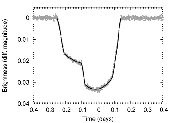
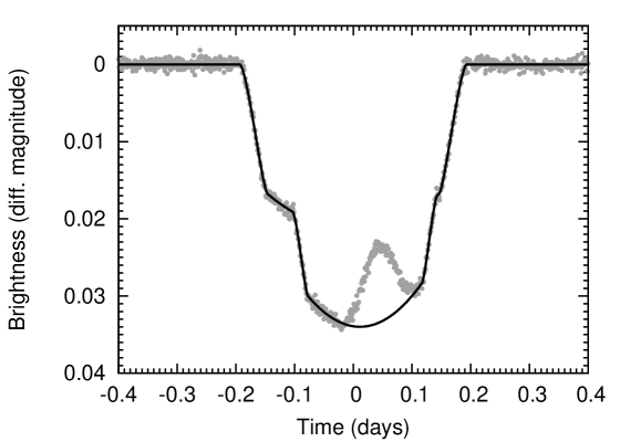
Figure 3: Simulated light curves of transits caused by two, relatively large planets and occurring nearly simultaneously but without any overlap (left panel). A light curve of a mutual transit with almost the same geometry is displayed on the right panel. The signal-to-noise ratio on these plots are nearly the same as one expects from Kepler photometry. The thick solid lines show the expected flux if the two simultaneous transits would be treated independently, i.e. the apparent overlapping of the planets would be neglected. See text for further details, including the geometric parameters of these simulated transits.

2.4.3 Linear limb darkening

The well known formula of linear limb darkening law gives us a surface flux density that can be written in the form of

$$I(x,y)=1-c[1-\mu],$$ (19)

where $\mu=\sqrt{1-x^{2}-y^{2}}$ and $c$ denotes the linear limb darkening coefficient. Performing integrals on this function will yield a linear combination of integrating a constant (see Section 2.4.1) and integrating the function $\sqrt{1-x^{2}-y^{2}}$. Thus, here we derive a function of which exterior derivative is $\sqrt{1-x^{2}-y^{2}}$ as well as we compute the indefinite integral that is going to appear in equation (7). First of all, we have to note that this function is defined only in the domain bounded by the circle $x^{2}+y^{2}=1$.

Let us search the function $\mathbf{f}$ of which exterior derivative is $\sqrt{1-x^{2}-y^{2}}\equiv\sqrt{1-r^{2}}$ in the form of $\mathbf{f}=\left[-yf(r^{2})/2,+xf(r^{2})/2\right]$. For simplicity, we introduce $r^{2}=x^{2}+y^{2}$. It is easy to show that the expansion of equation (4) for this function yields an ordinary differential equation (ODE) for $f(\cdot)$ that is

$$f(\xi)+\xi f^{\prime}(\xi)=\sqrt{1-\xi},$$ (20)

where $\xi=r^{2}$. One of the solutions of this ODE is

$$\frac{2}{3}\frac{1-(1-\xi)^{3/2}}{\xi}.$$ (21)

This solution behaves analytically at $\xi=0$, i.e. at the center of the stellar disk. Therefore, the function $\mathbf{f}$ can be written as

$$\mathbf{f}={f_{x}\choose f_{y}}=\frac{1-(1-x^{2}-y^{2})^{3/2}}{3(x^{2}+y^{2})}{-y\choose+x}.$$ (22)

By substituting this $\mathbf{x}=(f_{x},f_{y})$ into equation (7), one finds that the primitive integral

$$F[\varphi^{\prime}]=\frac{1}{3}\int\frac{1-(1-R^{2}-2r\rho\cos\varphi^{\prime})^{3/2}}{R^{2}+2r\rho\cos\varphi^{\prime}}(r+\rho\cos\varphi^{\prime})r\,\mathrm{d}\varphi^{\prime}$$ (23)

should be computed, if we parameterize the arc (on which the $\mathbf{f}$ is integrated) similarly as earlier. The constants are the following: $\rho^{2}=x_{0}^{2}+y_{0}^{2}$, $R^{2}=r^{2}+\rho^{2}$, and $\varphi^{\prime}$ is defined to be $\rho\cos\varphi^{\prime}$ equals to $x_{0}\cos\varphi+y_{0}\sin\varphi$. The primitive integral in equation (23) can be computed analytically and this computation yields a function which contains elementary functions as well as elliptic integrals. As a first step, let us introduce the constants

$$q_{2} = r^{2}+\rho^{2}+2r\rho\cos\varphi^{\prime},$$ (24)

$$s_{2} = (r+\rho)^{2},$$ (25)

$$d_{2} = (r-\rho)^{2},$$ (26)

$$Q = \frac{1}{\sqrt{r\rho}},$$ (27)

$$s_{\rm E} = 2\cos(\varphi^{\prime}/2)\sqrt{\frac{r\rho}{1-d_{2}}},$$ (28)

$$k_{\rm E} = \frac{1}{2}\sqrt{\frac{1-d_{2}}{r\rho}},$$ (29)

$$n_{\rm E} = -\frac{1-d_{2}}{d_{2}},$$ (30)

$$\hat{F} = \mathrm{F}(s_{\rm E};k_{\rm E}),$$ (31)

$$\hat{E} = \mathrm{E}(s_{\rm E};k_{\rm E}),$$ (32)

$$\hat{P} = \Pi(s_{\rm E};n_{\rm E},k_{\rm E}).$$ (33)

Here $\mathrm{F}(\cdot;\cdot)$, $\mathrm{E}(\cdot;\cdot)$ and $\Pi(\cdot;\cdot,\cdot)$ denotes the incomplete elliptic integrals of the first, second and third kind, respectively. Then, $F[\varphi^{\prime}]$ in equation (23) is computed as

$$F[\varphi^{\prime}] = -\frac{1}{3}\arctan\left[\sqrt{\frac{d_{2}}{s_{2}}}\tan\left(\frac{\varphi^{\prime}}{2}\right)\right]\frac{\rho^{2}-r^{2}}{\sqrt{d_{2}s_{2}}}+$$ (34)

$$+ \frac{\varphi^{\prime}}{6}+\frac{2}{9}r\rho\sqrt{1-q_{2}}\sin\varphi^{\prime}+$$

$$+ \frac{1}{6}(1-4r^{2}+2r^{4})Q\hat{F}+$$

$$+ \frac{1}{9}r\rho(7r^{2}+5r\rho+\rho^{2}-4)Q\hat{F}+$$

$$+ \frac{1}{9}r\rho(8-14r^{2}-2\rho^{2})Q\hat{E}+$$

$$+ \frac{1}{6}\frac{r+\rho}{r-\rho}Q\hat{P}.$$

One may note some similarities between these terms and the equations in Mandel & Agol (2002) or Pál (2008). Although the formulae above include incomplete elliptic integrals, the actual evaluation of these does not require longer computation time than the complete ones. Both types of elliptic integrals are computed via the Carlson symmetric forms (Carlson & Gustafson, 1993), for which computation very fast and robust algorithms are available in the literature (Press et al., 1992; Carlson, 1994).

It should also be noted that the evaluation of equation (34) might be done with caution in some cases where the values of the variables or constants defined in equations (24) - (33) introduce singularities in some of the terms. These values correspond to cases where the arc endpoints are at the edge of the bounding circle at $x^{2}+y^{2}=1$ and/or when the arc intersect the origin (i.e. if $x=y=0$). However, these singularities yield more simple formulae in general. For instance, the case of $\rho=0$ (i.e. when the bounding circle and the arc is concentric), equation (34) becomes simply

$$F[\varphi^{\prime}]=\frac{1}{3}\left[1-(1-r^{2})^{3/2}\right]\varphi^{\prime}.$$ (35)

Especially, when the arc is a part of the bounding circle itself (which is a practically frequent case: see e.g. the thick solid lines in the frames of Fig. 2), i.e. when $r=1$ and $\rho=0$, then $F[\varphi^{\prime}]$ is merely $\varphi^{\prime}/3$. All in all, these cases should be treated carefully during a practical implementation.

2.4.4 Quadratic limb darkening

The quadratic limb darkening stellar profile is characterized by the surface flux density $I=1-c_{1}(1-\mu)-c_{2}(1-\mu)^{2}$. Since $\mu=\sqrt{1-x^{2}-y^{2}}$, by expanding this equation, we obtain a constant term, with a value of $1-c_{1}-2c_{2}$, a polynomial term $x^{2}+y^{2}$ with a coefficient $+c_{2}$ and a term that is proportional to $\mu$ and has a coefficient $c_{1}+2c_{2}$. Hence, the formulae in the previous three subsections (2.4.1, 2.4.2 and 2.4.3) can be applied accordingly to evaluate the final apparent fluxes in the case of a quadratic limb darkening law.

3 Orbital inclinations

Mutual transits occur when at least two bodies (that can be, for instance, two planets or a planet and its moon) transits the host star simultaneously and their projections also overlap. Due to this overlap, the observed flux coming from the host star is larger than if we would consider naively the flux decreases from each body independently. In Fig. 2 we display a series of images that clearly show this effect. In the previous section we deduced the algorithms and mathematical formulae that are needed for the computation of the total observed flux for arbitrary geometry and for various limb darkening models.

As a demonstration, in Fig. 3 we display two simulated light curves with nearly the same orbital geometry. The planet-to-size ratio for the two companions are $R_{1}/R_{\star}=0.13$ and $R_{2}/R_{\star}=0.10$ while the orbital parameters are the following: $a_{1}/R_{\star}=4.3000$, $b_{1}=0.35$, $n_{1}=2.0\,{\rm d}^{-1}$, $a_{2}/R_{\star}=9.5952$, $b_{2}=0.22$, $n_{2}=0.6\,{\rm d}^{-1}$, $\Delta\Omega=18^{\circ}$ and both of the planets have a circular orbit. Here $n_{k}$ denotes the orbital angular frequency: it is $n_{k}=2\pi/P_{k}$, where $P_{k}$ is the orbital period. $b_{k}$ is the impact parameter of the transit, $a_{k}/R_{\star}$ is the normalized semimajor axis (in the units of stellar radii) and $\Delta\Omega=\Omega_{1}-\Omega_{2}$ is difference in the orbital ascending nodes (note that the reference plane here is the plane of the sky). The mid-transit time of the inner planet is $E_{1}=0.02\,{\rm d}$ while the outer planet has $E_{2}=-0.06\,{\rm d}$ on the left panel, and $E_{2}=0.00\,{\rm d}$ on the right panel. This difference between the mid-transit times yields a mutual transit in the latter case (see the flux excess in Fig. 3 at $t\approx 0.02\dots 0.08\,{\rm d}$) while there is no overlap between the apparent planetary disks in the former case.

It can easily be seen that the time evolution of the flux excess yielded by the mutual transit has similar qualitative properties as the normal transits have. Namely, it has a mid-time, a peak and a duration. The larger the flux excess peak, the larger the overlapping area is. At a first glance, the only quantity for which an observation of a mutual transit yields additional constraints is the difference in the $\Delta\Omega$, the difference between the orbital ascending nodes. Qualitatively, the longer the duration of this flux excess, the smaller the absolute value of $\Delta\Omega$ is. However, the depth and the exact time of the mutual event defines the impact parameters more precisely. This is rather relevant when one or both of the impact parameters are relatively small: the uncertainty of $b^{2}$ does not strongly depend on the actual value of $b$ (see e.g. Pál, 2008; Carter et al., 2008), thus the uncertainty in $b$ will be rather large for small values of $b$ due to the relation $\Delta b=(2b)^{-1}\Delta(b^{2})$. Indeed, for instance, the analysis of the light curves shown in Fig. 3 yields the following. If no mutual transit occurs (left panel), the best-fit values for $b_{k}$’s will be $b_{1}=0.323\pm 0.012$ and $b_{2}=0.215\pm 0.016$ while if we can observe the mutual transit, we obtain $b_{1}=0.351\pm 0.003$ and $b_{2}=0.223\pm 0.007$ while for the node difference we got $\Delta\Omega=17.4\pm 0.5^{\circ}$. For this demonstration of light curve analysis, we employed an improved Markov Chain Monte-Carlo algorithm as implemented in the lfit utility (Pál, 2009).

Of course, if the difference in the nodes, $\Delta\Omega=\Omega_{1}-\Omega_{2}$ is known, we can compute the mutual inclination $i_{\rm m}$ of the orbits as well using the well-known relation

$$\cos i_{\rm m}=\cos i_{1}\cos i_{2}+\sin i_{1}\sin i_{2}\cos\Delta\Omega.$$ (36)

It should also be mentioned that the analysis of mutual transits resolve the ambiguity between the values of $\pm\Delta\Omega$. And of course, the precise analysis of mutual transits should involve the gravitational interactions between the companions (see e.g. Pál, 2010), especially when data are available on a timescale on which the perturbations are not negligible (contrary to the demonstration presented here).

4 Discussion

In this paper we investigated the possibilities for computing apparent stellar fluxes in multiple or hierarchical stellar and/or planetary systems during simultaneous transits or occultations. The presented algorithm is capable to derive these fluxes for arbitrary number of bodies that are actively parts of the transiting or eclipsing event. This method can then be applied for various analyses of complex astrophysical systems, including multiple transiting planetary systems, hierarchical stellar systems with planetary companions and extrasolar moons as well.

Currently, the algorithm is implemented in ANSI C, in the form of a plug-in module for the program lfit and available from the address http://szofi.elte.hu/~apal/utils/astro/mttr/. This module features functions named mttrXy(.), where X denotes the number of transiting bodies and y can be “u”, “l” or “q” for the uniform flux density, linear limb darkening and quadratic limb darkening. Evidently, these functions have $3X+y$ parameters where $y$ is $0$, $1$ or $2$ for “u”, “l” or “q”, respectively. The current version of this module does not compute the parametric derivatives of the functions analytically but emulates them using numerical approximations for the lfit utility. Since both the parametric derivatives of the arcs (with respect to the circle center coordinates and radii) and the parametric derivatives of equation (7) can be computed analytically, the composition of these two would give us the required derivatives.

As a demonstration, we applied this method to obtain mutual inclinations of orbits in multiple transiting planetary systems. The analysis presented here clearly shows that observing a mutual transits yields not only an accurate value for the ascending node difference but also results a more precise value for the impact parameters, and therefore the orbital inclinations as well.

References

- Barge et al. (2008) Barge, P. et al. 2008, A&A, 482, 17
- Borucki et al. (2009) Borucki, W. J. et al. 2009, Science, 325, 709
- Borucki et al. (2011) Borucki, W. J. et al. 2011, ApJ, 736, 19
- Carlson & Gustafson (1993) Carlson, B. C. & Gustafson, J. L. 1993, e-print (arXiv:math/9310223)
- Carlson (1994) Carlson, B. C. 1994, e-print (arXiv:math/9409227)
- Carter et al. (2008) Carter, J. A., Yee, J. C., Eastman, J., Gaudi, B. S. & Winn, J. N. 2008, ApJ, 689, 499
- Doyle et al. (2011) Doyle, L. R. et al. 2011, Science, 333, 1602
- Giménez (2006) Giménez, A., 2006, A&A, 450, 1231
- Holman (2010) Holman, M. J. et al. 2010, Science, 330, 51
- Kipping (2009) Kipping, D., 2009, MNRAS, 392, 181
- Kipping (2011) Kipping, D., 2011, MNRAS, 416, 689
- Lissauer et al. (2011) Lissauer, J. et al. 2011, Nature, 470, 53
- Mandel & Agol (2002) Mandel, K. & Agol, E., 2002, ApJ, 580, 171
- Pál (2008) Pál, A. 2008, MNRAS, 390, 281
- Pál (2009) Pál, A. 2009, PhD thesis (arXiv:0906.3486)
- Pál (2010) Pál, A. 2010, MNRAS, 409, 975
- Press et al. (1992) Press, W. H., Teukolsky, S. A., Vetterling, W.T., Flannery, B.P., 1992, Numerical Recipes in C: the art of scientific computing, Second Edition, Cambridge University Press
- Ragozzine & Holman (2010) Ragozzine, D. & Holman, M. J. 2010, ApJ, submitted (arXiv:1006.3727)
- Sato & Asada (2009) Sato, M. & Asada, H. 2009, PASJ, 61, 29
- Simon et al. (2009) Simon, A. E., Szabó, Gy. M. & Szatmáry, K. 2009, EM&P, 105, 385
- Szabó et al. (2006) Szabó, Gy. M., Szatmáry, K.; Divéki, Zs. & Simon, A. 2006, A&A, 450, 395
- Szabó et al. (2011) Szabó, Gy. M. et al. 2011, ApJ, 736, 4