Transverse Momentum Dependent Fragmentation and Quark Distribution Functions from the NJL-jet Model

Abstract

Using the model of Nambu and Jona-Lasinio to provide a microscopic description of both the structure of the nucleon and of the quark to hadron elementary fragmentation functions, we investigate the transverse momentum dependence of the unpolarized quark distributions in the nucleon and of the quark to pion and kaon fragmentation functions. The transverse momentum dependence of the fragmentation functions is determined within a Monte Carlo framework, with the notable result that the average $P_{\perp}^{2}$ of the produced kaons is significantly larger than that of the pions. We also find that $\langle P_{\perp}^{2}\rangle$ has a sizable $z$ dependence, in contrast with the naive Gaussian ansatz for the fragmentation functions. Diquark correlations in the nucleon give rise to a nontrivial flavor dependence in the unpolarized transverse-momentum-dependent quark distribution functions. The $\langle k_{T}^{2}\rangle$ of the quarks in the nucleon are also found to have a sizable $x$ dependence. Finally, these results are used as input to a Monte Carlo event generator for semi-inclusive deep inelastic scattering (SIDIS), which is used to determine the average transverse momentum squared of the produced hadrons measured in SIDIS, namely, $\langle P_{T}^{2}\rangle$. Again, we find that the average $P_{T}^{2}$ of the produced kaons in SIDIS is significantly larger than that of the pions and in each case $\langle P_{T}^{2}\rangle$ has a sizable $z$ dependence.

I Introduction

Semi-inclusive deep inelastic scattering (SIDIS) has a very rich structure which provides a wealth of observables far in excess of the familiar inclusive deep inelastic scattering (DIS). The 2-dimensional picture of a target provided by SIDIS promises many new insights into nucleon and nuclear structure Collins:1977iv; Ralston:1979ys; Collins:1984kg; Mulders:1995dh. For example, it has been realized that SIDIS may shed light on the angular momentum structure of the proton in terms of the spin and orbital angular momentum of its quarks and gluons Bacchetta:2011gx; Avakian:2010br; She:2009jq. It will also provide new information on the in-medium modification of bound nucleons and deepen our understanding of QCD itself Collins:1977iv; Ralston:1979ys; Collins:1984kg; Mulders:1995dh. The study of the transverse momentum distribution of hadrons produced in SIDIS Collins:1977iv; Ralston:1979ys; Collins:1984kg; Mulders:1995dh; Boer:1997nt; Collins:2007ph; Bacchetta:2007wc; Amrath:2005gv is characterized by determining the transverse-momentum-dependent (TMD) parton distribution functions (PDFs) and the TMD fragmentation functions.

Early theoretical models of the fragmentation functions have been constructed in Refs. Bacchetta:2002tk; Pasquini:2011tk; Jakob:1997wg; Kitagawa:2000ji; Yang:2002gh and more recently the development of the NJL-jet model Ito:2009zc has provided a framework which automatically satisfies the relevant sum rules. Lattice QCD studies of TMD PDFs are presented in Ref. Musch:2010ka and the QCD evolution of TMD PDFs is discussed in Ref. Aybat:2011zv. Extensive phenomenological data analysis of transverse momentum in distribution and fragmentation processes was presented in Ref. Schweitzer:2010tt. Considerable experimental work has already been carried out at JLab Avakian:2003pk; Osipenko:2008rv; Mkrtchyan:2007sr; Avakian:2010ae; Asaturyan:2011mq, HERMES Airapetian:2004tw; Airapetian:2009jy; Airapetian:2009ti and COMPASS Alexakhin:2005iw; Ageev:2006da; Rajotte:2010ir, while for an overview of the future perspectives for this field we refer to the recent review by Anselmino et al. Anselmino:2011ay.

In this work, we present the first microscopic calculation of the spin–independent TMD quark distribution functions in the nucleon and the TMD quark to pion and kaon fragmentation functions, where none of the parameters are adjusted to TMD data. The underlying theoretical framework is the Nambu–Jona-Lasinio (NJL) model Nambu:1961tp; Nambu:1961fr. While this certainly represents a simplification of QCD, it has many desirable properties. For example, it is covariant and respects the chiral symmetry of QCD, including its dynamical breaking. Moreover, it describes the spin and flavor dependence of the nucleon PDFs, as well as their modification in-medium Cloet:2005pp; Cloet:2005rt; Cloet:2006bq. It also produces transversity quark distributions Cloet:2007em which are in good agreement with the empirical distributions extracted by Anselmino et al. Anselmino:2007fs.

For the present purpose the recent developments in the NJL-jet model Ito:2009zc; Matevosyan:2010hh; Matevosyan:2011ey, which provides a quark-jet description of the fragmentation process using elementary fragmentation functions calculated within the standard NJL model, are also critical. This framework provides a good description of the parametrizations of experimental data and has been extended to include vector meson resonances and nucleons as fragmentation channels. The use of Monte Carlo methods to calculate these fragmentation functions has also been implemented and that development allows us to address a wider array of processes within the model, including physical cross-section calculations.

In Sec. II, we present the general formalism for describing transverse momentum distributions in SIDIS, including the quark-jet model originally proposed by Field and Feynman. The calculation of the elementary, unintegrated fragmentation functions in the NJL model, which are the input to the jet model which describes the TMD fragmentation functions in quark hadronization, is explained in Sec. III. Our model for the TMD quark distribution functions in the nucleon is outlined in Sec. IV, where we also present results for the TMD PDFs. Results for the TMD fragmentation functions are discussed in Sec. V and the average transverse momentum in the SIDIS process, determined using our Monte Carlo event generator, is discussed in Sec. VI. Finally, Sec. VII contains a summary and outlook.

II Transverse Momentum in the NJL-jet Model

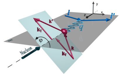
Figure 1: Illustration of the three-dimensional kinematics of SIDIS. The photon momentum defines the $z$ axis and the struck quark has initial transverse momentum $\bm{k_{T}}$ in the nucleon, with respect to the $z$ axis.

The kinematics of semi-inclusive hadron production, $lN\to l^{\prime}hX$, is illustrated schematically in Fig. 1, where a lepton with momentum $l$ scatters on a target, by emitting a virtual photon with momentum $q$ that hits a quark with initial momentum $k$. As usual, the $z$ axis is chosen to coincide with the direction of the photon’s momentum, where the target has its momentum in the negative $z$ direction. The transverse momenta in the process – labeled with a subscript $T$ – are defined with respect to this $z$ axis, so that the photon and target have no transverse momentum component ($\gamma N$ collinear kinematics). The angle between the lepton scattering plane and the quark scattering plane is denoted as $\varphi$. We allow for the struck quark in the target to carry a transverse momentum $\bm{k_{T}}$. Some of this transverse momentum is then transferred to the hadrons emitted by the quark.

The kinematics of the quark fragmentation process is depicted in Fig. 2. The emitted hadron $h$ carries a transverse momentum $\bm{P_{T}}$ with respect to the $z$ axis which can be decomposed into two contributions. First, the quark transfers a fraction of its transverse momentum $\bm{k_{T}}$ to the hadron and second the hadron also acquires a momentum transverse to the direction of the quark’s momentum, $\bm{P_{\perp}}$. Up to corrections of order $\mathcal{O}(k_{T}^{2}/Q^{2})$, the following relation holds Anselmino:2005nn:

$$\bm{P_{T}}=\bm{P_{\perp}}+z\,\bm{k_{T}}.$$ (1)

This relation allows one to probe the quark transverse momentum inside a nucleon by measuring the $z$ dependence of the emitted hadron’s transverse momentum $\langle P_{T}^{2}\rangle$, provided $\langle P_{\perp}^{2}\rangle$ is independent of $z$. However, in the NJL-jet model framework we find that $\langle P_{\perp}^{2}\rangle$ is strongly $z$ dependent and this $z$ dependence is also observed at COMPASS Rajotte:2010ir. A recent analysis of the HERMES data Airapetian:2009jy was performed in Ref. Schweitzer:2010tt, where a Gaussian ansatz for the TMD quark distribution and fragmentation functions was assumed and an average was performed over the quark flavor and type of hadron detected. Using a fit region of $0.2<z<0.7$, they extracted the following results for the average transverse momentum squared Schweitzer:2010tt:

$$\langle k_{T}^{2}\rangle=0.38\pm 0.06\ \mathrm{GeV}^{2},$$ (2)

$$\langle P_{\perp}^{2}\rangle=0.16\pm 0.01\ \mathrm{GeV}^{2}.$$ (3)

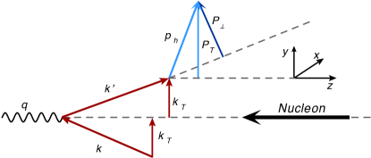
Figure 2: Illustration of the kinematics of SIDIS, where the final transverse momentum of the produced hadron with respect to the $z$ axis is denoted by $\textbf{\em P}_{\textbf{\em T}}$, which is related to the initial quark transverse momentum in the nucleon $\textbf{\em k}_{\textbf{\em T}}$ and that generated in the fragmentation process $\textbf{\em P}_{\mathbf{\perp}}$ by Eq. (1).

The latest iteration of the NJL-jet model Matevosyan:2011ey employs Monte Carlo simulations to calculate the integrated quark fragmentation functions. It assumes that the initial high energy quark emits hadrons in a cascade-like process, schematically depicted in Fig. 3. At every emission vertex we choose the type of emitted hadron $h$ and its fraction of the light-cone momentum $z$ of the fragmenting quark, by randomly sampling the corresponding elementary quark fragmentation (splitting) functions, $\hat{d}_{q}^{h}(z)$, that are calculated within the NJL model. In each elementary fragmentation process we record the flavor of the initial and final quarks and the type of the emitted hadron, we also note the light-cone momentum fraction of the initial quark transferred to the hadron and that left to the final quark. The fragmentation chain is stopped after the quark has emitted a predefined number of hadrons, $N_{Links}$. We repeat the calculation $N_{Sims}$ times, with the same initial quark flavor, $q$, until we have sufficient statistics for the emitted hadrons. The fragmentation functions are then extracted by calculating the average number of hadrons of type $h$, with light-cone momentum fraction $z$ to $z+\Delta z$, which we denote by $\left<N_{q}^{h}(z,z+\Delta z)\right>$. The fragmentation function in the domain $[z,z+\Delta z]$ is then given by

$$D_{q}^{h}(z)\Delta z=\left<N_{q}^{h}(z,z+\Delta z)\right>\equiv\frac{\sum_{N_{Sims}}N_{q}^{h}(z,z+\Delta z)}{N_{Sims}}.$$ (4)

In this work, we extend the NJL-jet model to include the transverse momentum dependence of the emitted hadrons in the fragmentation process. This is achieved by using TMD elementary quark fragmentation functions at the hadron emission vertices and by keeping track of the transverse momenta of all the particles in the process. Our goal is to calculate the TMD fragmentation function, $D_{q}^{h}(z,P_{\perp}^{2})$, using its probabilistic interpretation. That is, the probability of a quark $q$ to emit a hadron $h$ with a fraction $z$ of its light-cone momentum and a transverse momentum $\bm{P_{\perp}}$ is given by $D_{q}^{h}(z,P_{\perp}^{2})\,dz\,d^{2}\bm{P}_{\perp}$.

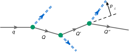
Figure 3: NJL-jet model including transverse momentum.

We calculate elementary (one-step) TMD splitting functions, $\hat{d}_{q}^{h}(z,p_{\perp}^{2})$, using the NJL model, where $\bm{p_{\perp}}$ denotes the transverse component of the hadron’s momentum with respect to the parent quark, as illustrated in Figs. 3 and 4. In each step of the Monte Carlo simulation of the quark cascade emission, we randomly sample the type, the light-cone momentum fraction, $z$, and the transverse momentum, $\bm{p_{\perp}}$, of the emitted hadron using as the probability distribution the elementary TMD splitting functions of the quark, where the elementary probability is $\hat{d}(z,p_{\perp}^{2})\,dz\,d^{2}\bm{p}_{\perp}$. Schematically, the quark emission process is depicted in Fig. 4, where the $z^{\prime}$ axis denotes the direction of the original parent quark’s 3-momentum. The vectors $\bm{k}$ and $\bm{k^{\prime}}$ denote the 3-momentum of an arbitrary quark in the cascade chain before and after hadron emission with transverse components $\bm{k_{\perp}}$ and $\bm{k^{\prime}_{\perp}}$, respectively. The emitted hadron’s momentum is labeled by $\bm{p_{h}}$, where its transverse component with respect to $\bm{k}$ and the $z^{\prime}$ axis is denoted by $\bm{p_{\perp}}$ and $\bm{P_{\perp}}$, respectively. $\bm{P_{\perp}}$ is obtained using the relation $\bm{P_{\perp}}=\bm{p_{\perp}}+z\,\bm{k_{\perp}}$, analogous to that in Eq. (1). The recoil transverse momentum of the final quark, $\bm{k^{\prime}_{\perp}}$, is calculated from momentum conservation in the transverse plane, namely,

$$\bm{k_{\perp}}=\bm{P_{\perp}}+\bm{k^{\prime}_{\perp}}.$$ (5)

The TMD fragmentation function is then calculated after the trivial integration over the polar angle of $\bm{P}_{\perp}$ in the transverse plane, that is

$$D_{q}^{h}(z,P_{\perp}^{2})\,\Delta z\,\pi\Delta P_{\perp}^{2}=\left<N_{q}^{h}(z,z+\Delta z,P_{\perp}^{2},P_{\perp}^{2}+\Delta P_{\perp}^{2}\right>$$

$$\hskip 34.1433pt\equiv\frac{\sum_{N_{Sims}}N_{q}^{h}(z,z+\Delta z,P_{\perp}^{2},P_{\perp}^{2}+\Delta P_{\perp}^{2})}{N_{Sims}}.$$ (6)

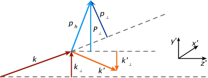
Figure 4: Quark elementary fragmentation kinematics, for an arbitrary hadron emission in the cascade chain. The $z^{\prime}$ axis is defined by the direction of the 3-momentum of the original parent quark.

The model can easily accommodate the initial transverse momentum of the quark, for example, with respect to the direction of the virtual photon in SIDIS (see Fig. 1). Our goal is to describe the average transverse momentum of the hadrons produced in different reactions. The differential cross section for SIDIS up to terms of order $\mathcal{O}(k_{T}^{2}/Q^{2})$ can be written as Anselmino:2005nn

$$\frac{d^{3}\sigma^{lN\to l^{\prime}hX}}{dx\ dz\ dP_{T}^{2}} \sim\sum_{q}e^{2}_{q}\int d^{2}\bm{k_{T}}\ q(x,k_{T}^{2})\ D_{q}^{h}(z,P_{\perp}^{2})$$

$$\equiv\sum_{q}\,e_{q}^{2}\,\widetilde{D}_{q}^{h}(x,z,P_{T}^{2}),$$ (7)

where $\bm{P}_{\perp}$ and $\bm{P_{T}}$ are related by Eq. (1) and $q(x,k_{T}^{2})$ are the TMD quark distribution functions of the target. Thus for SIDIS, we can use the TMD quark distribution functions to randomly sample the initial transverse momentum of the quark to calculate the relevant number density of the produced hadrons. In this work, we use TMD valence quark distributions in the nucleon – calculated within the NJL model – to determine the average transverse momentum of the produced hadrons with respect to the direction of the virtual photon, that is $\langle P_{T}^{2}\rangle$, by calculating the corresponding probability densities $\widetilde{D}_{q}^{h}(x,z,P_{T}^{2})$, using an expression analogous to Eq. (6). In this way, we obtain a self-consistent description of the entire process in the regime where the virtual photon samples the valence quark component of the target, that is, when the struck quark has $x\gtrsim 0.3$. The type of target and the allowed range of $x$ in the Monte Carlo simulation can be matched to those measured in any particular experiment.

In this article, we only consider the production of pseudoscalar mesons, that is, the pions and kaons, as a first step in determining the TMD fragmentation functions. Eventually, we will also include the vector mesons and nucleon-antinucleon channels, as done for the integrated fragmentation functions in Ref. Matevosyan:2011ey.

III Elementary TMD Fragmentation Functions

In this section, we evaluate the “elementary” fragmentation functions of quarks to hadrons as a “one-step” process in the NJL model, using light-cone coordinates. The NJL model which we use includes only four point quark interactions in the Lagrangian, with up, down and strange quarks (see, for example, Refs. Kato:1993zw; Klimt:1989pm; Klevansky:1992qe for detailed reviews of the NJL model). In the present work, we use the notation introduced in our previous studies Matevosyan:2010hh; Matevosyan:2011ey.

The elementary fragmentation function for quark, $q$, to emit a meson, $m$, carrying light-cone momentum fraction, $z$, and carrying transverse momentum, $p_{\perp}$, is depicted in Fig. 5. In the frame where the fragmenting quark has zero transverse momentum, but a nonzero transverse momentum component $-\bm{p_{\perp}}/z$ with respect to the direction of the produced hadron Collins:1977iv; Ito:2009zc, the unregularized elementary TMD fragmentation functions to pseudoscalar mesons are given by

$$d_{q}^{m}(z,p_{\perp}^{2}) =-\frac{C_{q}^{m}}{2}\,g_{mqQ}^{2}\,\frac{z}{2}\int\frac{dk_{+}dk_{-}}{(2\pi)^{4}}\ \mathrm{Tr}\left[S_{1}(k)\gamma^{+}S_{1}(k)\gamma_{5}(\not{k}-\not{p}+M_{2})\gamma_{5}\right]\delta(k_{-}-p_{-}/z)\ 2\,\pi\,\delta\!\left((p-k)^{2}-M_{2}^{2}\right)$$

$$=\frac{C_{q}^{m}}{16\pi^{3}}\,g_{mqQ}^{2}\,z\ \frac{p_{\perp}^{2}+\left[(z-1)M_{1}+M_{2}\right]^{2}}{\left[p_{\perp}^{2}+z(z-1)M_{1}^{2}+zM_{2}^{2}+(1-z)m_{m}^{2}\right]^{2}}.$$ (8)

The trace is over Dirac indices only and the subscripts on the quark propagator, $S_{1}(k)$, and constituent masses, $M_{1}$ and $M_{2}$, denote quark flavors. Quark flavor is also indicated by the subscripts $q$ and $Q$, where a meson of type $m$ has the quark flavor structure $m=q\overline{Q}$ and $m_{m}$ denotes the meson mass. The corresponding isospin factor and quark-meson coupling constant are labeled by $C_{q}^{m}$ and $g_{mqQ}$, respectively, and are determined within the NJL model Matevosyan:2010hh; Matevosyan:2011ey. The integrated elementary splitting function is obtained from the elementary TMD splitting function via integration over $\bm{p}_{\perp}$, that is,

$$d_{q}^{m}(z)=\int d^{2}\bm{p}_{\perp}\ d_{q}^{m}(z,p_{\perp}^{2})=\frac{C_{q}^{m}}{2}g_{mqQ}^{2}\ z$$

$$\times\int\frac{d^{2}\bm{p}_{\perp}}{(2\pi)^{3}}\frac{p_{\perp}^{2}+\left[(z-1)M_{1}+M_{2}\right]^{2}}{\left[p_{\perp}^{2}+z(z-1)M_{1}^{2}+zM_{2}^{2}+(1-z)m_{m}^{2}\right]^{2}}.$$ (9)

The probability densities $\hat{d}_{q}^{m}(z)$ are then obtained by multiplying a normalization factor so that $\sum_{m}\int_{0}^{1}dz\,\hat{d}_{q}^{m}(z)=1$. The isospin and momentum sum rules are then satisfied automatically Matevosyan:2010hh; Matevosyan:2011ey.

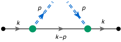
Figure 5: Feynman diagram describing the elementary quark to hadron fragmentation functions.

Previously, we employed the Lepage-Brodsky (LB) regularization scheme to calculate loop integrals such as that in Eq. (III). This method puts a sharp cutoff on the invariant mass squared, $M_{12}^{2}$, of the particles in the final state (see Refs. Bentz:1999gx; Ito:2009zc; Matevosyan:2010hh; Matevosyan:2011ey for a detailed description as applied to the NJL-jet model). The maximum invariant mass of the two particles in the loop, $\Lambda_{12}$, is determined by

$$M_{12}^{2}\leq\Lambda_{12}^{2}\equiv\left(\sqrt{\Lambda_{3}^{2}+\mu_{1}^{2}}+\sqrt{\Lambda_{3}^{2}+\mu_{2}^{2}}\right)^{2},$$ (10)

where $\mu_{1}$ and $\mu_{2}$ denote the masses of the particles in the loop and $\Lambda_{3}$ denotes the 3-momentum cutoff, which is fixed in the usual way by reproducing the experimental pion decay constant. For a light constituent quark mass of $M=0.4~{}\mathrm{GeV}$, the corresponding 3-momentum cutoff is $\Lambda_{3}=0.59~{}{\rm GeV}$. The strange constituent quark mass is determined by reproducing the experimental kaon mass, giving the value $M_{s}=0.61~{}\mathrm{GeV}$ and the corresponding quark-meson coupling constants are $g_{\pi qQ}=4.23$ and $g_{KqQ}=4.51$.

In loop integrals containing two particles, we assign a light-cone momentum fraction $x$ (of the initial particle’s light-cone momentum) to the particle with mass $\mu_{1}$ and consequently a light-cone momentum fraction $1-x$ for the particle with mass $mu_{2}$. Then, in the frame where the initial particle’s transverse momentum is zero, the invariant mass of the two particles in the loop can be expressed as

$$M_{12}^{2}=\frac{\mu_{1}^{2}+p_{\perp}^{2}}{x}+\frac{\mu_{2}^{2}+p_{\perp}^{2}}{1-x}.$$ (11)

The relation in Eq. (10), when applied to the integral in Eq. (III), yields a sharp cutoff in the integral over the transverse momentum, namely

$$p_{\perp}^{2}\leqslant\mathcal{P}_{\perp}^{2}\equiv z(1-z)\left[\sqrt{\Lambda_{3}^{2}+\mu_{1}^{2}}+\sqrt{\Lambda_{3}^{2}+\mu_{2}^{2}}\right]^{2}\\ -(1-z)\,\mu_{1}^{2}-z\,\mu_{2}^{2}.$$ (12)

A consequence of LB regularization is that it restricts the corresponding regularized functions to a limited range of $z$, namely $0<z_{min}\leqslant z\leqslant z_{max}<1$, where $z_{min}$ and $z_{max}$ are determined by imposing the condition $\mathcal{P}_{\perp}^{2}\geqslant 0$ in Eq. (12). These range limitations depend on the masses of hadrons and quarks involved. For example, the $z$ limits are very close to the endpoints ($z=0$ and $z=1$) for quark splitting functions to pions, but are further from these endpoints for heavier hadrons like kaons. The plots depicted in Fig. 6 show the limited range for the normalized splitting functions of a $u$ quark to $\pi^{+}$ and $K^{+}$, calculated using LB regularization.

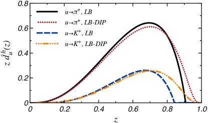
Figure 6: The normalized integrated splitting functions for a $u$ quark to $\pi^{+}$ and $K^{+}$, calculated using LB and LB-DIP regularizations with the same light constituent quark mass of $M=0.4\,\mathrm{GeV}$.

In this work, we employ a slightly modified version of the LB regularization, which replaces the sharp cutoff of the invariant mass squared in the integrals, namely, $\Theta(\Lambda_{12}^{2}-M_{12}^{2})$, by a dipole regulator:

$$G_{12}(p_{\perp}^{2})\equiv\frac{1}{\left[1+(M_{12}^{2}/\Lambda_{12}^{2})^{2}\right]^{2}}.$$ (13)

A physical motivation for this regularization scheme is that it gives a pion quark distribution that at large $x$ behaves approximately as $(1-x)^{2.6}$ for $Q^{2}=16\,$GeV², which is in good agreement with the recent reanalysis of Aicher et al. which finds $(1-x)^{2.34}$ at the same scale Aicher:2010cb. Using this dipole cutoff version of the LB regularization scheme (LB-DIP), we fix the model parameters by reproducing the experimentally measured hadronic properties, such as $f_{\pi}$ and the kaon mass to determine the cutoff as $\Lambda_{3}=0.773~{}\mathrm{GeV}$ and the strange constituent quark mass becomes $M_{s}=0.59~{}\mathrm{GeV}$. The corresponding quark-meson coupling constants are $g_{\pi qQ}=4.24$ and $g_{KqQ}=4.52$. The quark distribution functions calculated with LB-DIP regularization satisfy both the number and momentum sum rules and allow us to set the model scale at $Q_{0}^{2}=0.2~{}\mathrm{GeV^{2}}$ in the usual way by comparing the evolved pion distribution function with that obtained from experiment. This procedure is discussed in detail in Ref. Matevosyan:2010hh.

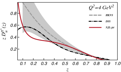
(a)

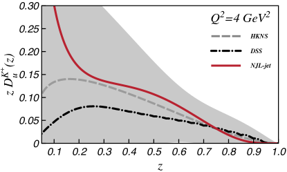
(b)

Figure 7: The integrated fragmentation functions for a $u$ quark to $\pi^{+}$ (upper) and $K^{+}$ (lower), calculated using the LB-DIP regularization with a light constituent quark mass of $M=0.4\,\mathrm{GeV}$ and evolved from the model scale to $Q^{2}=4\,\mathrm{GeV}^{2}$. The results are compared to phenomenological parametrizations of experimental data from Ref. Hirai:2007cx (HKNS) and Ref. deFlorian:2007aj (DSS). The shaded area represents the uncertainties in the HKNS results.

The plots in Fig. 6 clearly show that the $z$ range of the splitting functions calculated using LB-DIP allows for a smooth continuation of the corresponding splitting functions calculated using LB regularization to the endpoints $z=0$ and $z=1$. The plots in Fig. 7 present results for the fragmentation functions of a $u$ quark to $\pi^{+}$ and $K^{+}$ using the LB-DIP regularization scheme. We use the QCD evolution code of Ref. Botje:2010ay at next-to-leading order to evolve our model results from the scale $Q_{0}^{2}=0.2\,$GeV² to $Q^{2}=4\,$GeV². We find a slightly better description of the empirical parametrizations compared to our earlier work Matevosyan:2011ey; Matevosyan:2010hh, especially in the region where $z$ is close to $1$. Previously, artifacts of the LB regularization did not allow a good description in this domain.

IV TMD Quark Distributions in the Nucleon

The TMD quark distributions in the nucleon are again determined by utilizing the NJL model. The nucleon bound state is described by a relativistic Faddeev equation that includes both scalar and axial–vector diquark correlations, where the static approximation is used to truncate the quark exchange kernel Cloet:2005pp. The relevant terms of the NJL interaction Lagrangian are

$$\mathcal{L}_{I}=G_{s}\Bigl{(}\overline{\psi}\,\gamma_{5}C\tau_{2}\beta^{A}\,\overline{\psi}^{T}\Bigr{)}\Bigl{(}\psi^{T}\,C^{-1}\gamma_{5}\tau_{2}\beta_{A}\,\psi\Bigr{)}$$

$$+\,G_{a}\left(\overline{\psi}\,\gamma_{\mu}C\tau_{i}\tau_{2}\beta^{A}\,\overline{\psi}^{T}\right)\Bigl{(}\psi^{T}\,C^{-1}\gamma^{\mu}\tau_{2}\tau_{i}\beta_{A}\,\psi\Bigr{)},$$ (14)

where $C=i\gamma_{2}\gamma_{0}$ and $\beta_{A}=\sqrt{\tfrac{3}{2}}\,\lambda_{A}~{}~{}(A\in 2,5,7)$ are the color $\bar{3}$ matrices Cloet:2005pp. The strength of the scalar and axial–vector diquark correlations in the nucleon are determined by the couplings $G_{s}$ and $G_{a}$, respectively. To regularize the NJL model for the calculation of the nucleon, we choose the proper-time scheme, with an infrared and ultraviolet cutoff, labeled by $\Lambda_{IR}$ and $\Lambda_{UV}$, respectively. This scheme enables the removal of unphysical thresholds for nucleon decay into quarks, and hence simulates an important aspect of confinement Ebert:1996vx; Hellstern:1997nv; Bentz:2001vc. This simulation of quark confinement has also been shown to provide a natural saturation mechanism for nuclear matter in the NJL model Bentz:2001vc.

The proper-time regularization scheme is not used for the fragmentation functions because the emitted hadrons are not confined. Therefore, the confining nature of the proper-time regularization is not appropriate in this case. However, for consistency between both regularization schemes we use the same light constituent quark mass and fix the UV cutoff so as to reproduce the pion decay constant.

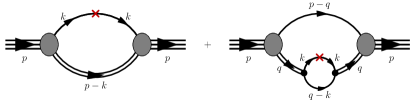
Figure 8: Feynman diagrams which give the unpolarized TMD quark distribution functions in the nucleon. The single line represents the quark propagator and the double line the diquark $t$-matrix. The shaded oval denotes the quark-diquark vertex function, obtained from a relativistic Faddeev equation and the operator insertion has the form $\gamma^{+}\delta(x-\tfrac{k^{+}}{p^{+}})\tfrac{1}{2}\left(1\pm\tau_{3}\right)$.

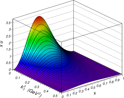
(a)

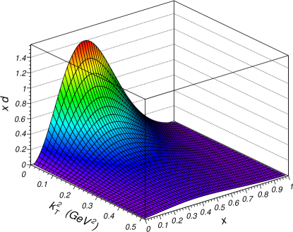
(b)

Figure 9: Results for the $u$ (upper) and $d$ (lower) TMD quark distributions in the proton.

The five parameters of our NJL model for the nucleon are the light constituent quark mass, $M$, the regularization parameters $\Lambda_{IR}$ and $\Lambda_{UV}$, and the couplings $G_{s}$ and $G_{a}$. These are determined by fixing $M=0.4\,$GeV, $\Lambda_{IR}=0.24\,$GeV, and then reproducing the nucleon mass, pion decay constant, and the nucleon axial coupling via Bjorken sum Cloet:2006bq; Cloet:2009qs. Strange quarks are not yet included in our model for the nucleon.

The leading-twist spin-independent TMD distribution of the quarks of flavor $q$ in the nucleon is defined via the correlator Bacchetta:2008af; Avakian:2010br

$$\mathcal{Q}(x,\bm{k_{T}})=p^{+}\int\frac{d\xi^{-}d\bm{\xi}_{T}}{(2\pi)^{3}}\ e^{ix\,p^{+}\,\xi^{-}}\,e^{-i\,\bm{k_{T}}\cdot\bm{\xi_{T}}}\\ \times\left\langle N,S\left|\bar{\psi}_{q}(0)\,\gamma^{+}\,\mathcal{W}(\xi)\,\psi_{q}(\xi^{-},\xi_{T})\right|N,S\right\rangle\Bigr{|}_{\xi^{+}=0},$$ (15)

where $\mathcal{W}(\xi)$ is a gauge link connecting the two quark fields, which are labeled by $\psi_{q}$. In QCD this gauge link is nontrivial for $\bm{\xi_{T}}\neq 0$, however at the level of approximation that we are working at, this gauge link equals unity in the NJL model. Our states are normalized using the noncovariant light-cone normalization, namely

$$\sideset{}{{}_{q}}{\sum}\left\langle N,S\left|\bar{\psi}_{q}(0)\,\gamma^{+}\,\psi_{q}(0)\right|N,S\right\rangle=3.$$ (16)

Equation (15) can be expressed in terms of two TMD quark distribution functions, namely,

$$\mathcal{Q}(x,\bm{k_{T}}) =q(x,k_{T}^{2})-\frac{\varepsilon^{-+ij}\,k_{T}^{i}\,S_{T}^{j}}{M}\,q_{1T}^{\perp}(x,k_{T}^{2}),$$ (17)

where the first TMD PDF integrated over $\bm{k_{T}}$ gives the familiar unpolarized quark distribution function and the second TMD PDF, known as the Sivers function Sivers:1989cc; Bacchetta:2003rz, is time-reversal odd and is zero at the level of approximation included in this work.

To determine the TMD quark distributions in this model, it is convenient to express them in the form Jaffe:1985je; Barone:2001sp

$$q(x,\,k_{T}^{2})=-i\int\frac{dk^{+}dk^{-}}{(2\pi)^{4}}\delta\!\left(x-\frac{k^{+}}{p^{+}}\right)\text{Tr}\left[\gamma^{+}\,M_{q}(p,k)\right],$$ (18)

where $M_{q}(p,k)$ is the quark two-point function in the bound nucleon. Therefore, within any model that describes the nucleon as a bound state of quarks, the quark distribution functions can be associated with a straightforward Feynman diagram calculation.

The Feynman diagrams considered here are given in Fig. 8, where the first diagram represents the so–called quark diagram and the second the diquark diagram. The single line in each diagram represents a quark propagator which is the solution to the gap equation and the double line is the diquark $t$-matrix obtained from the Bethe–Salpeter equation. The vertex functions represent the solution to the nucleon Faddeev equation. The resulting distributions have no support for negative $x$ and therefore this is essentially a valence quark picture. By separating the isospin factors, the spin-independent $u$ and $d$ TMD quark distributions in the proton can be expressed as

$$u(x,k_{T}^{2}) =f^{s}_{q/N}(x,k_{T}^{2})+\tfrac{1}{3}\,f^{a}_{q/N}(x,k_{T}^{2})$$

$$+\tfrac{1}{2}\,f^{s}_{q(D)/N}(x,k_{T}^{2})+\tfrac{5}{6}\,f^{a}_{q(D)/N}(x,k_{T}^{2}),$$ (19)

$$d(x,k_{T}^{2}) =\tfrac{2}{3}\,f^{a}_{q/N}(x,k_{T}^{2})$$

$$+\tfrac{1}{2}\,f^{s}_{q(D)/N}(x,k_{T}^{2})+\tfrac{1}{6}\,f^{a}_{q(D)/N}(x,k_{T}^{2}).$$ (20)

The superscripts $s$ and $a$ refer to the scalar and axial-vector terms, respectively, the subscript $q/N$ implies a quark diagram and $q(D)/N$ a diquark diagram. Explicit expressions for the functions in Eqs. (IV) and (IV) are given in the Appendix.

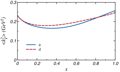
Figure 10: The Bjorken $x$ dependence of $\left<k_{T}^{2}\right>$. Diquark correlations in the nucleon give rise to the quark flavor dependence.

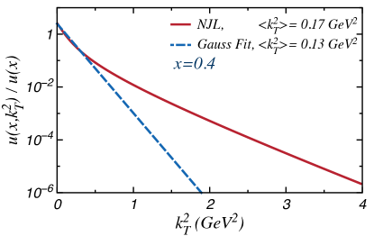
(a)

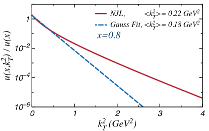
(b)

Figure 11: Results for the TMD $u$-quark distribution in the proton for fixed $x$ slices, where the upper plot has $x=0.4$ and the lower plot is for $x=0.8$. Also plotted are individual fits to the TMD quark distribution using the Gaussian ansatz of Eq.(21) for each $x$, with $\langle k_{T}^{2}\rangle$ the single fit parameter in each case.

Results for the $u$- and $d$-quark TMD quark distributions functions in the proton are illustrated in Fig. 9. The $Q^{2}$ scale to which these results correspond is not determined by the model. Previously for the familiar spin-independent PDFs we fitted the valence $u$-quark distribution in the proton to the empirical result at some large $Q^{2}$ scale, this gives a model scale of $Q_{0}^{2}=0.16\,$GeV² Cloet:2005pp; Cloet:2006bq; Cloet:2007em in the proper-time regularization scheme. Rigorous comparison with the experimental data requires QCD evolution of the model TMD PDFs, which is left for future work. Here, we just show the results as they emerge from our model, the exact scale of which is not so important for this purpose. When QCD evolution is included, both the TMD PDF and TMD fragmentation function model scales must be equal when determining observables like SIDIS cross–sections. The integral of these TMD PDF results over $\bm{k_{T}}$ gives the familiar spin-independent quark distributions functions, which satisfy the baryon number and momentum sum rules. The Bjorken $x$ and $k_{T}^{2}$ dependence in these expressions is not separable, and therefore the Gaussian ansatz for the TMD quark distributions, namely, that they can be written in the form

$$q(x,\,k_{T}^{2})=q(x)\ \frac{e^{-k_{T}^{2}/\left<k_{T}^{2}\right>}}{\pi\,\left<k_{T}^{2}\right>},$$ (21)

is not possible for our TMD PDF results. The Bjorken $x$ dependence of $\left<k_{T}^{2}\right>$ for our proton TMD quark distribution results is illustrated in Fig. 10, where

$$\left<k_{T}^{2}\right>(x)\equiv\frac{\int d^{2}\bm{k_{T}}\ k_{T}^{2}\,q(x,\,k_{T}^{2})}{\int d^{2}\bm{k_{T}}\ q(x,\,k_{T}^{2})}.$$ (22)

If the $x$ and $k_{T}^{2}$ dependence of our TMD quark distributions were separable then the curves in Fig. 10 would be constants, however we find that $\left<k_{T}^{2}\right>$ has about a $20\%$ variation over the domain of Bjorken $x$. We also find that the $x$ dependence of $\left<k_{T}^{2}\right>$ for the $u$ and $d$ quarks differs somewhat, with the $d$ quarks having slightly larger $\left<k_{T}^{2}\right>$ for the majority of Bjorken $x$.

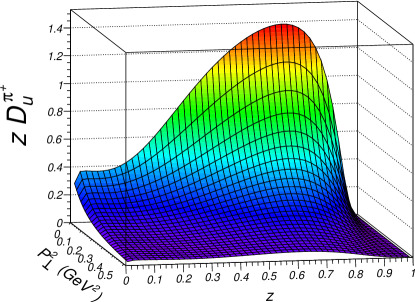
(a)

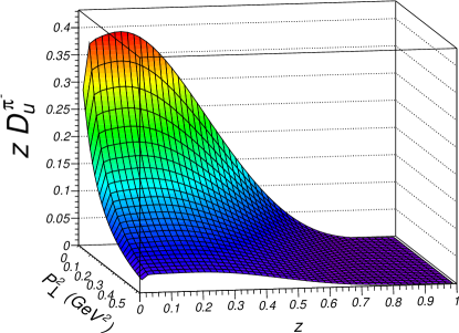
(b)

Figure 12: TMD fragmentation functions for a $u$ quark to $\pi^{+}$ and $\pi^{-}$. The upper figure illustrates the favored case, which peaks at relatively large $z$, while the unfavored case, shown in the lower figure, peaks at much smaller $z$.

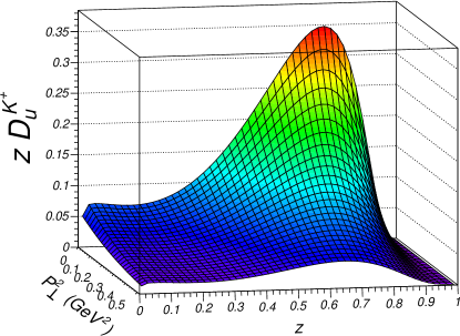
(a)

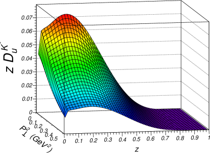
(b)

Figure 13: TMD fragmentation functions for a $u$ quark to $K^{+}$ and $K^{-}$. The upper figure illustrates the favored case, which peaks at relatively large $z$, while the unfavored case, shown in the lower figure, peaks at much smaller $z$.

Figure 11 illustrates our TMD quark distribution results at particular $x$ values and compares them to a Gaussian ansatz fit for the same $x$ slice. The Gaussian ansatz results are obtained by a least squares fit of the TMD factor in Eq. (21) to our ratios $q(x,k_{T}^{2})/q(x)$ calculated in the NJL model, using $\langle k_{T}^{2}\rangle$ of Eq. (21) as the only fit parameter for each value of $x$. The fitted value of this parameter is approximately 20% smaller than the value of $\langle k_{T}^{2}\rangle$ calculated with our model distribution functions. In the least squares fit, we included values of $k_{T}^{2}$ up to $4\,$GeV² and the curves in Fig. 11 indicate that such a fit to a single Gaussian is reasonable only for a limited $k_{T}^{2}$ region, for a single value of $x$.

V TMD Fragmentation Function Results

In this section, we present NJL-jet model results for the TMD fragmentation functions. The number of emitted hadrons in the decay chain is set to $N_{Links}=6$, which is sufficient to accurately obtain the pion and kaon fragmentation functions in the domain $z\gtrsim 0.02$. We solve for the fragmentation of $u$, $d$, and $s$ quarks to pions and kaons, utilizing Monte Carlo simulations and the expression in Eq. (6), similar to our previous calculations of the integrated fragmentation functions detailed in Ref. Matevosyan:2011ey. The computational challenge for the Monte Carlo simulations is to obtain sufficient statistics and this becomes significantly more difficult when we include the transverse momentum dependence, because now the number of bins becomes quadratic in the size of the discrete bin size (taken to be $1/500$ both for $z$ and transverse momentum, in the corresponding units). Furthermore, the extent of the bins in the transverse momentum direction was extended to $6~{}\mathrm{GeV}^{2}$, in order to avoid any notable numerical artifacts arising from the limited range of transverse momentum. To overcome the numerical challenge, our software platform was developed to allow for parallel generation of the Monte Carlo quark decay cascades, with different seeds for their random number generators. The results were later combined to produce the high statistics solutions. The computations were facilitated on the small computer cluster at the Special Research Centre for the Subatomic Structure of Matter (CSSM) that consists of 11 machines with Intel Core i7 920 quad core CPUs running on the Linux Fedora Core 11 operating system and GCC 4.4. A typical calculation of fragmentation for a given quark type takes about $12$ hours with $44$ parallel processors.

Results for the TMD favored and unfavored fragmentation functions for a $u$ quark to $\pi$ and $K$ mesons are illustrated in Figs. 12 and 13. In each case, the favored TMD fragmentation functions have more support at large $z$, while the unfavored results are peaked at smaller $z$. It is also evident that the kaon fragmentation functions fall off more slowly in $P_{\perp}^{2}$ than the corresponding pion fragmentation functions. The drop in each of the fragmentation functions for $z\lesssim 0.02$ is a consequence of choosing $N_{Links}=6$, which means that in the Monte Carlo simulation there is a vanishingly small probability of emitting hadrons with $z<0.02$.

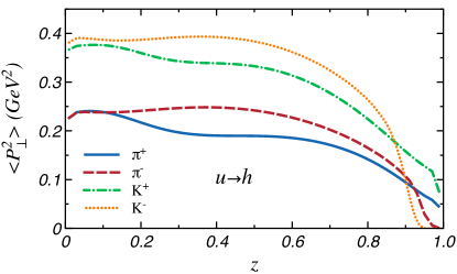
Figure 14: The averaged transverse momentum of $\pi$ and $K$ mesons emitted by a $u$ quark.

The Gaussian ansatz is widely used to describe the traverse momentum dependence of both quark distribution and fragmentation functions. In particular, the TMD fragmentation function of a quark $q$ emitting a hadron $h$ is often modeled by

$$D_{q}^{h}(z,P_{\perp}^{2})=D_{q}^{h}(z)\frac{e^{-P_{\perp}^{2}/\langle P_{\perp}^{2}\rangle}}{\pi\langle P_{\perp}^{2}\rangle},$$ (23)

where $D_{q}^{h}(z)$ is the corresponding integrated fragmentation function and $\langle P_{\perp}^{2}\rangle$ is the average transverse momentum of the produced hadron $h$, defined by

$$\langle P_{\perp}^{2}\rangle(z)\equiv\frac{\int d^{2}\bm{P_{\perp}}\ P_{\perp}^{2}\,D_{q}^{h}(z,P_{\perp}^{2})}{\int d^{2}\bm{P_{\perp}}\ D_{q}^{h}(z,P_{\perp}^{2})}.$$ (24)

In analyses that assume a Gaussian ansatz for the TMD fragmentation functions, it is usual to assume that $\langle P_{\perp}^{2}\rangle$ does not depend on $z$, the type of hadron, $h$, or the quark flavor, $q$. These assumptions will be tested against the NJL-jet TMD fragmentation functions.

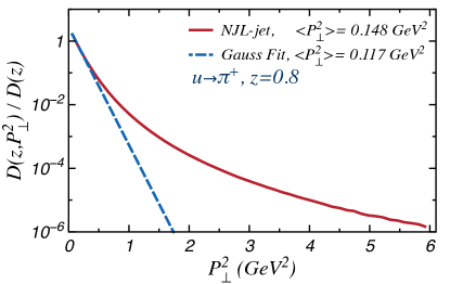
(a)

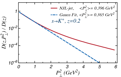
(b)

Figure 15: Normalized TMD fragmentation for the favored $u\to\pi^{+}$ process for $z=0.8$ (upper) and the unfavored $s\to K^{+}$ process for $z=0.2$ (lower). Also depicted are fits to the fragmentation functions using the Gaussian ansatz of Eq. (23), with $\langle P_{\perp}^{2}\rangle$ as the single fitting parameter.

The results in Fig. 14 depict the average transverse momenta of $\pi$ and $K$ mesons produced by a $u$-quark. These plots show that the average transverse momenta of the hadrons are relatively flat versus $z$ in the region $0.3<z<0.6$, however they have a significant dependence on the type of the hadron. We find that the average transverse momentum of the kaons is significantly larger than that of the pions.

The curves in Fig. 15 depict the TMD fragmentation of a favored $u\to\pi^{+}$ process for $z=0.8$ and an unfavored $s\to K^{+}$ process for $z=0.2$. Also presented are least squares fits to the fragmentation functions for particular $z$ slices using the Gaussian ansatz of Eq. (23), with $\langle P_{\perp}^{2}\rangle$ the single fitting parameter for each $z$. The plots in Fig. 15 indicate that such a fit to a single Gaussian is reasonable only for a limited $P_{\perp}^{2}$ region. Also, because $\langle P_{\perp}^{2}\rangle$ has a significant $z$ dependence, the Gaussian ansatz for the entire TMD fragmentation function offers at best a crude approximation to the full results. The corresponding average transverse momenta obtained from the Gaussian fits are smaller than those obtained directly using the relation in Eq. (24).

VI Average Transverse Momenta in SIDIS

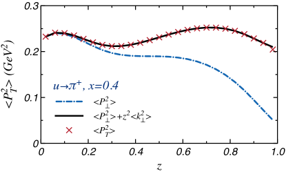
Figure 16: The averaged transverse momentum of $\pi^{+}$ mesons in SIDIS produced on a $u$ quark in a proton with light-cone momentum fraction $x=0.4$.

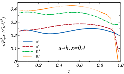
Figure 17: The averaged transverse momentum of $\pi$ and $K$ mesons in SIDIS on a $u$ quark in the proton with light-cone momentum fraction $x=0.4$. The unfavored fragmentation functions rapidly approach zero for large $z$ and this causes the dramatic changes in $\langle P_{T}^{2}\rangle$ at large $z$ illustrated in this figure.

For the SIDIS process we have created a Monte Carlo event generator that can calculate the physical cross-section. In future work this will enable us to analyze the relative importance of the different aspects of the process and the implications of the constraints set in individual experiments. We use it to determine the average transverse momentum of the produced hadrons (at the model scale) observed in a SIDIS experiment, namely $\langle P_{T}^{2}\rangle$, which is defined as

$$\langle P_{T}^{2}\rangle(x,z)\equiv\frac{\int d^{2}\bm{P_{T}}\ P_{T}^{2}\,\widetilde{D}_{q}^{h}(x,z,P_{T}^{2})}{\int d^{2}\bm{P_{\perp}}\ \widetilde{D}_{q}^{h}(x,z,P_{T}^{2})}.$$ (25)

The function $\widetilde{D}_{q}^{h}(x,z,P_{T}^{2})$ is defined in Eq. (II). The crosses in Fig. 16 represent results for $\langle P_{T}^{2}\rangle$ acquired by $\pi^{+}$ mesons in a SIDIS hadronization process, where the virtual photon strikes a valence $u$ quark in a proton carrying a light-cone momentum fraction of $x=0.4$. We also plot as the dash-dotted line $\langle P_{\perp}^{2}\rangle$, which is the average transverse momentum that the $\pi^{+}$ mesons acquire in the quark fragmentation process. Recall, that the transverse momentum $\bm{P_{\perp}}$ is defined relative to the direction of the original fragmenting quark, while $\bm{P_{T}}$ is relative to the direction of the photon momentum, these transverse momenta are related by Eq. (1). For the factorization of the SIDIS cross–section given in Eq. (II), it can be shown that $\langle P_{T}^{2}\rangle$ is given by

$$\langle P_{T}^{2}\rangle(x,z)=\langle P_{\perp}^{2}\rangle(z)+z^{2}\langle k_{T}^{2}\rangle(x).$$ (26)

As an additional check on the Monte Carlo calculation, in Fig. 16 we plot the result obtained from Eq. (26) as the solid line and find that it agrees perfectly with that obtained from the Monte Carlo event generator for the SIDIS cross–section. We also find that both $\langle P_{\perp}^{2}\rangle$ and $\langle P_{T}^{2}\rangle$ illustrated in Fig. 16 have a sizable $z$ dependence.

Illustrated in Fig. 17 are results for the average transverse momentum acquired by $\pi$ and $K$ mesons in the hadronization process in SIDIS, where the struck quark is a $u$ quark in a proton with light-cone momentum fraction $x=0.4$. The rapid approach to zero for the unfavored fragmentation functions in Fig. 17 is a consequence of the large $z$ behavior of the unfavored $\langle P_{\perp}^{2}\rangle$ illustrated in Fig. 14, which also rapidly approach zero. The HERMES experimental results for $\langle P_{T}^{2}\rangle$ measured in SIDIS on a deuterium target Airapetian:2009jy, are of comparable size to our results shown in Fig. 17. We do not plot these HERMES results because the kinematic range is too different for a quantitative comparison. The average transverse momentum of the kaons is larger than that of the pions at the low $Q^{2}$ scale of the model. Our model includes only the valence quarks in the proton, which should be the dominant component at $x=0.4$.

VII Conclusions and Outlook

In this work we extended the NJL-jet model to include the transverse momentum dependence in the quark hadronization process. This was achieved using TMD elementary fragmentation functions and by keeping track of the quark’s recoil transverse momentum in the hadron emission cascade. We modified the LB regularization scheme to remove artifacts that limit the $z$ range of the splitting functions, and this in turn improved our description of the integrated fragmentation functions. The TMD fragmentation functions for $u$, $d$, and $s$ quarks to pions and kaons were determined using a Monte Carlo approach. The average $P_{\perp}^{2}$ of the produced kaons was found to be significantly larger than that of the pions and in both cases $\langle P_{\perp}^{2}\rangle$ had a sizable $z$ dependence. The high statistical precision needed for these calculations was achieved through parallel computing on the small computer farm at CSSM.

The TMD quark distribution functions in the proton were also determined using the NJL model. In this case, we used the proper-time regularization scheme, because this method simulates important aspects of confinement. Our TMD PDF results when integrated over $\bm{k_{T}}$ give our earlier results for the familiar spin-independent quark distribution functions Cloet:2005pp, whose moments satisfy the baryon number and momentum sum rules. We found that the average $k_{T}^{2}$ of the quarks in the nucleon have a significant $x$ dependence and therefore the familiar Gaussian ansatz for the TMD PDFs produces only a crude approximation to our full TMD PDF results.

Finally, using the TMD quark distribution functions for the nucleon and the results for the TMD fragmentation functions, we constructed a Monte Carlo event generator for the SIDIS process. Using this Monte Carlo event generator, we determined the average transverse momentum of the hadrons, $\langle P_{T}^{2}\rangle$, produced in SIDIS. These results are of a similar magnitude to those extracted from experiment, even at our relatively low model scale. As a cross check for this SIDIS Monte Carlo event generator, we compared our results for $\langle P_{T}^{2}\rangle$ with those obtained using Eq. (26), finding perfect agreement. We find that the $\langle P_{T}^{2}\rangle$ of the produced kaons is significantly larger than that of the pions, which is not apparent in the current experimental measurements.

An interesting extension of our model would be to include the vector meson and nucleon antinucleon emission channels. This extension has already been completed in our previous work on the integrated fragmentation functions. It would also be intriguing to consider the spin-dependent effects in the hadronization process, in particular, to calculate the Collins fragmentation function. Further, using the NJL description of nucleon structure we will be able to develop a self-consistent description of the spin-dependent effects in SIDIS reactions.

APPENDIX: Nucleon TMD PDF expressions

The $u$ and $d$ valence TMD quark distribution functions in the proton are given by

$$u_{v}(x,k_{T}^{2}) =f^{s}_{q/N}(x,k_{T}^{2})+\tfrac{1}{3}\,f^{a}_{q/N}(x,k_{T}^{2})$$

$$+\tfrac{1}{2}\,f^{s}_{q(D)/N}(x,k_{T}^{2})+\tfrac{5}{6}\,f^{a}_{q(D)/N}(x,k_{T}^{2}),$$ (27)

$$d_{v}(x,k_{T}^{2}) =\tfrac{2}{3}\,f^{a}_{q/N}(x,k_{T}^{2})$$

$$+\tfrac{1}{2}\,f^{s}_{q(D)/N}(x,k_{T}^{2})+\tfrac{1}{6}\,f^{a}_{q(D)/N}(x,k_{T}^{2}).$$ (28)

The individual quark diagrams terms have the form

$$f_{q/N}^{s}(x,k_{T}^{2})=\frac{\alpha_{1}^{2}\,Z_{N}\,Z_{s}}{16\pi^{3}}\left(1-x\right)\int d\tau\,\left[1+\tau\,x\left[\left(M_{N}+M\right)^{2}-m_{s}^{2}\right]\right]e^{-\tau\left[k_{T}^{2}+x\left(x-1\right)M_{N}^{2}+x\,m_{s}^{2}+\left(1-x\right)M^{2}\right]},$$ (29)

$$f_{q/N}^{a}(x,k_{T}^{2})=-\frac{Z_{a}\,Z_{N}}{16\pi^{3}}\,(1-x)$$

$$\int d\tau\,\left[\left(\alpha_{2}^{2}-2\alpha_{2}\alpha_{3}-2\alpha_{3}^{2}\right)\left(1+\tau\,x\,\left[(M_{N}-M)^{2}-m_{a}^{2}\right]\right)-12\alpha_{3}^{2}\,\tau\,x\,M\,M_{N}\right]e^{-\tau\left[k_{T}^{2}+x\left(x-1\right)M_{N}^{2}+x\,m_{a}^{2}+\left(1-x\right)M^{2}\right]},$$ (30)

and the diquark diagrams terms are given by

$$f^{s}_{q(D)/N}(x,k_{T}^{2}) =\iint_{0}^{1}dy\,dz\ \delta\!\left(x-yz\right)f^{s}_{q/D}(z,k_{T}^{2})\ f^{s}_{q/N}(1-y),$$ (31)

$$f^{a}_{q(D)/N}(x,k_{T}^{2}) =\iint_{0}^{1}dy\,dz\ \delta\!\left(x-yz\right)f^{a}_{q/D}(z,k_{T}^{2})\ f^{a}_{q/N}(1-y).$$ (32)

The diquark TMD quark distributions are

$$f^{s}_{q/D}(x,k_{T}^{2}) =\frac{3\,Z_{s}}{4\pi^{3}}\,\int d\tau\,\left[1+\tau\,x\,(1-x)\,m_{s}^{2}\right]e^{-\tau\left[k_{T}^{2}+x(x-1)\,m_{s}^{2}+M^{2}\right]},$$ (33)

$$f^{a}_{q/D}(x,k_{T}^{2}) =\frac{3\,Z_{a}}{\pi^{3}}\,x(1-x)\int\,d\tau\,\left[1+\tau\,x(1-x)m_{a}^{2}\right]e^{-\tau\left[k_{T}^{2}+x(x-1)m_{a}^{2}+M^{2}\right]}.$$ (34)

The constituent quark, scalar diquark, axial–vector diquark, and nucleon masses in these expressions have the values $M=0.4\,$GeV, $m_{s}=0.687\,$GeV, $m_{a}=1.03\,$GeV, and $M_{N}=0.94\,$GeV. The weight factors in the nucleon Faddeev vertex Mineo:1999eq; Mineo:2002bg; Cloet:2005pp and its normalization are given by $\left(\alpha_{1},\,\alpha_{2},\,\alpha_{3}\right)=\left(0.429,\,0.0244,\,-0.445\right)$ and $Z_{N}=29.9$, respectively. Finally the pole residues of the scalar and axial–vector diquark $t$-matrices are $Z_{s}=14.5$ and $Z_{a}=3.82$, respectively. Integrating over $\bm{k_{T}}$ in these expressions gives the familiar spin-independent quark distribution functions, the moments of which satisfy the baryon number and momentum sum rules.

These expressions have been derived using the proper-time regularization scheme, which in practice means to make the substitution

$$\frac{1}{X^{n}}=\frac{1}{(n-1)!}\int_{0}^{\infty}d\tau\ \tau^{n-1}e^{-\tau X}\\ \longrightarrow\frac{1}{(n-1)!}\int_{1/\Lambda_{UV}^{2}}^{1/\Lambda_{IR}^{2}}d\tau\ \tau^{n-1}e^{-\tau X},$$ (35)

where $X$ denotes the denominator function in a loop integral after Feynman parameterization and Wick rotation. The infrared and ultraviolet cutoffs have the values $\Lambda_{IR}=0.240\,$GeV and $\Lambda_{UV}=0.645\,$GeV, respectively.