Spontaneous chiral symmetry breaking in the Tayler instability

Abstract

The chiral symmetry breaking properties of the Tayler instability are discussed. Effective amplitude equations are determined in one case. This model has three free parameters that are determined numerically. Comparison with chiral symmetry breaking in biochemistry is made.

1 Introduction

An important ingredient to the solar dynamo is the $\alpha$ effect. Mathematically speaking $\alpha$ is a pseudo scalar that can be constructed using gravity $\textstyle g$ (a polar vector) and angular velocity $\textstyle\Omega$ (an axial vector): $\mathchoice{\mbox{\boldmath$\displaystyle g$}}{\mbox{\boldmath$\textstyle g$}}{\mbox{\boldmath$\scriptstyle g$}}{\mbox{\boldmath$\scriptscriptstyle g$}}{}\cdot\mathchoice{\mbox{\boldmath$\displaystyle\Omega$}}{\mbox{\boldmath$\textstyle\Omega$}}{\mbox{\boldmath$\scriptstyle\Omega$}}{\mbox{\boldmath$\scriptscriptstyle\Omega$}}{}$ is thus a pseudo scalar and is proportional to $\cos\theta$, where $\theta$ is the colatitude. This pseudo scalar changes sign at the equator. This explanation for large-scale astrophysical dynamos works well and therefore one used to think that the existence of the $\alpha$ effect in dynamo theory requires always the existence of a pseudo scalar in the problem. This has indeed been general wisdom, although it has rarely been emphasized in the literature. That this is actually not the case has only recently been emphasized and demonstrated. One example is the magnetic buoyancy instability in the absence of rotation, but with a horizontal magnetic field $\textstyle B$ and vertical gravity $\textstyle g$ being perpendicular to each other, so the pseudo scalar $\mathchoice{\mbox{\boldmath$\displaystyle g$}}{\mbox{\boldmath$\textstyle g$}}{\mbox{\boldmath$\scriptstyle g$}}{\mbox{\boldmath$\scriptscriptstyle g$}}{}\cdot\mathchoice{\mbox{\boldmath$\displaystyle B$}}{\mbox{\boldmath$\textstyle B$}}{\mbox{\boldmath$\scriptstyle B$}}{\mbox{\boldmath$\scriptscriptstyle B$}}{}$ vanishes (Chatterjee et al., 2011). Another example is the Tayler instability of a purely toroidal field in a cylinder (Gellert et al., 2011). Thus, the magnetic field is again perpendicular to all possible polar vectors that can be constructed, for example the gradient of the magnetic energy density which points in the radial direction. In both cases, kinetic helicity and a finite $\alpha$, both of either sign, emerge in the nonlinear stage of the instability. In the former case, the $\alpha$ tensor has been computed using the test-field method. In the latter, the components of the $\alpha$ tensor have been computed using the imposed-field method (see Hubbard et al., 2009, for a discussion of possible pitfalls in the nonlinear case).

The purpose of the present paper is to examine spontaneous chiral symmetry breaking in the Tayler instability and to estimate numerically the coefficients governing the underlying amplitude equations. This allows us then to make contact with a model system of chemical reactions that can give rise to the same type of spontaneous symmetry breaking.

The connection with chemical systems is of interest because the question of spontaneous symmetry breaking has a long history ever since Pasteur (1853) discovered the preferential handedness of certain organic molecules. The preferential handedness of biomolecules is believed to be the result of a bifurcation event that took place at the origin of life itself (Kondepudi & Nelson, 1984; Sandars, 2003; Brandenburg et al., 2005).

2 Numerical simulations

Our setup consists of an isothermal cylinder with a radial extent from $s_{\rm in}$ to $s_{\rm out}$ and vertical size $h$. We solve the time dependent ideal MHD equations with periodic boundary conditions in $z$, reflection in $s$ and periodic in $\varphi$ and a resolution ranging from $64^{3}$ to $128^{3}$ in the three directions.

The azimuthal field in the basic state is taken of the form

$$B_{\varphi}=b_{0}\;(s/s_{0})\exp[-(s-s_{0})^{2}/\sigma^{2}]$$

with $b_{0}$ being a normalization constant; the axial field $B_{z}$ is chosen to be zero. In the basic state, the Lorentz force is balanced with a gradient of pressure, and we have checked that our setup was numerically stable if no perturbation was introduced in the system. For the actual calculations we have chosen $h=2$, $s_{\rm in}=1$, $s_{\rm out}=3$, $s_{0}=2$ and $\sigma^{2}=0.2$. The sound speed is assumed to be much larger than the Alfén speed ($\approx$ ten times), similar to what happens in stellar interiors.

At the beginning of the simulation we perturb the magnetic field. We add a perturbation of amplitude $10^{-7}$ that of the background field. The perturbing field has a given helicity that is either positive or negative. During the development of the instability we observe a net increase of the helicity, as shown in Fig. 1 where we plot time series of the normalized magnetic helicity, which exhibits an initial exponential growth, reaches a peak and then levels off.

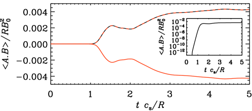
Figure 1: Evolution of magnetic helicity for two initial conditions. differing only in the parity of their initial perturbations. After the exponential growth magnetic helicity levels off. In the inset a detail of the exponential growth phase. Here, $R\equiv s_{\rm in}$ is used.

3 Amplitude equations

The linear stability analysis of this instability shows that there exists helical growing modes. But the left handed and right handed modes have exactly the same growth rate independent of their helicity. Hence the growth of helical perturbations cannot be described by a linear theory. However a weakly nonlinear theory is able to describe it as we show below. Let us begin by considering two helical modes of right handed and left handed variety respectively each of which satisfy the Beltrami relation ${\bm{\nabla}}\times\bm{R}=\Lambda\bm{R}$ and ${\bm{\nabla}}\times\bm{L}=-\Lambda\bm{L}$ . We can deal with the Fourier transform of these modes, given by

$$\bm{L}({\bm{x}})=\int\hat{\bm{L}}({\bm{q}})d^{d}q\quad\mbox{and}\quad\bm{R}({\bm{x}})=\int\hat{\bm{R}}({\bm{q}})d^{d}q$$ (1)

For the left helical mode, total helicity and energy are given by

$$E_{L}=\frac{1}{2}\int\bm{L}^{2}({\bm{x}})d^{d}x=\frac{1}{2}\int\hat{\bm{L}}\cdot\hat{\bm{L}}^{\ast}d^{d}q\quad\mbox{and}\quad\mathcal{H}_{L}=\int\bm{L}\cdot{\bm{\nabla}}\times\bm{L}d^{d}x=-2\Lambda E_{L},$$ (2)

where $\ast$ denotes complex conjugation. We then have $E=E_{L}+E_{R}$ being the total energy and $\mathcal{H}=\mathcal{H}_{L}+\mathcal{H}_{R}$ the total helicity. An analogous relation holds for the right-handed helical mode too.

In the weakly nonlinear regime the evolution of these modes can be described by general equations of the form:

$$\frac{\partial\hat{\bm{L}}}{\partial t}=\frac{\delta\mathcal{L}}{\delta\hat{\bm{L}}}\quad\mbox{and}\quad\frac{\partial\hat{\bm{R}}}{\partial t}=\frac{\delta\mathcal{L}}{\delta\hat{\bm{R}}},$$ (3)

where the Lagrangian $\mathcal{L}$ can often by written down from symmetry considerations. In the present case one has to consider the fact that under parity transformation $L$ can $R$ interchanges into each other. With this additional symmetry the simplest Lagrangian takes the following form (Fauve et al., 1991)

$$\mathcal{L}[\hat{\bm{L}},\hat{\bm{R}}]=\int\gamma\left[|\hat{\bm{L}}|^{2}+|\hat{\bm{R}}|^{2}\right]-\mu\left[|\hat{\bm{L}}|^{4}+|\hat{\bm{R}}|^{4}-\mu_{\ast}|\hat{\bm{L}}|^{2}|\hat{\bm{R}}|^{2}d^{d}q\right]d^{d}q,$$ (4)

The coefficients $\gamma$, $\mu$ and $\mu_{\ast}$ cannot be found from symmetry considerations. Note that in order to show the simplest form, in writing down the Lagrangian we have ignored dissipation. This gives rise to the following set of amplitude equations,

$$\frac{\partial\hat{\bm{L}}}{\partial t}=\gamma\hat{\bm{L}}-\left(\mu|\hat{\bm{L}}|^{2}+\mu_{\ast}|\hat{\bm{R}}|^{2}\right)\hat{\bm{L}},\quad\frac{\partial\hat{\bm{R}}}{\partial t}=\gamma\hat{\bm{R}}-\left(\mu|\hat{\bm{R}}|^{2}+\mu_{\ast}|\hat{\bm{L}}|^{2}\right)\hat{\bm{R}}.$$ (5)

For certain range of parameters these coupled equations allow the growth of one mode at the expense of the other (Fauve et al., 1991), a phenomenon known to biologists by the name “mutual antagonism” (Frank, 1953).

Using Eqs. (2) and (5) and defining $H=\mathcal{H}/{2\Lambda}$ we can obtain evolution equations for $E$ and $H$ as

$$\frac{dE}{dt} = 2\gamma E-2(\mu+\mu_{\ast})E^{2}-2(\mu-\mu_{\ast})H^{2},$$ (6)

$$\frac{dH}{dt} = 2\gamma H-4\mu EH.$$ (7)

Hence, by calculating the total energy and helicity from direct numerical simulations (DNS) we can determine the unknown coefficients $\gamma,\mu$ and $\mu_{\ast}$.

To determine the coefficients $\gamma$, $\mu$, and $\mu_{*}$, we define the instantaneous logarithmic time derivatives of $E$ and $H$, $\gamma_{E}={\textstyle{1\over 2}}{\rm d}{}\ln E/{\rm d}{}t$ and $\gamma_{H}={\textstyle{1\over 2}}{\rm d}{}\ln H/{\rm d}{}t$, so we have

$$\gamma=\gamma_{H}+2\mu E,\quad\mu=(\gamma-\gamma_{H})/2E,\quad\mu_{*}=[(\gamma-\gamma_{E})E-\mu(E^{2}+H^{2})]/(E^{2}-H^{2}).$$ (8)

The result is shown in Fig. 2, where we can identify first the value of $\gamma\approx 14$ during the initial linear growth phase of the instability, and then the values $\mu\approx 10$ and $\mu_{*}\approx 7$ during the nonlinear stage.

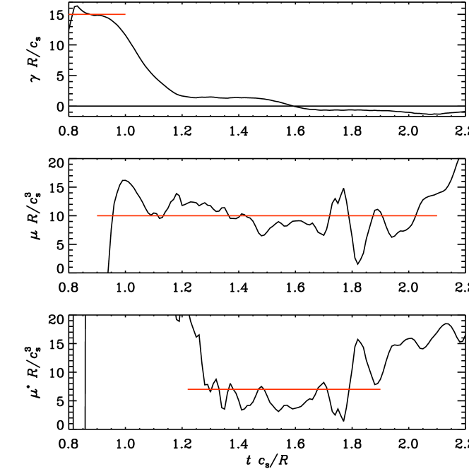
Figure 2: Time dependence of $\gamma$, $\mu$, and $\mu_{8}$, normalized in terms inner radius and sound speed. The red lines give the fit results $\gamma\approx 14$, $\mu\approx 10$, and $\mu^{*}\approx 7$ in the appropriate units.

4 Conclusions

The present work has demonstrated that the Tayler instability can produce parity-breaking and that it is possible to determine empirical fit parameters that reproduce the nonlinear evolution of energy and helicity. So far, no rigorous derivation of the amplitude equations exists, so this would be an important next step. Comparing with the chiral symmetry breaking instabilities in biochemistry, an important difference is that in the present equations the nonlinearity is always cubic, while in biochemistry the dominant nonlinearity tends to be quadratic. In this light, it would be useful to assess more closely the possible differences between biochemical and magnetohydrodynamical symmetry breaking.

References

- Brandenburg et al. (2005) Brandenburg, A., Andersen, A. C., Höfner, S., & Nilsson, M., Orig. Life Evol. Biosph. 35, 225 (2005).
- Chatterjee et al. (2011) Chatterjee, P., Mitra, D., Brandenburg, A., & Rheinhardt, M., Phys. Rev. E 84, 025403R (2011).
- Frank (1953) Frank, F. C., Biochim. Biophys. Acta 11, 459 (1953).
- Gellert et al. (2011) Gellert, M., Rüdiger, G., & Hollerbach, R., Mon. Not. R. Astron. Soc. 414, 2696 (2011).
- Fauve et al. (1991) Fauve, S., Douady, S., & Thual, O., J. Phys. II 1, 311 (1991).
- Hubbard et al. (2009) Hubbard, A., Del Sordo, F., Käpylä, P. J., & Brandenburg, A., Mon. Not. R. Astron. Soc. 398, 1891 (2009).
- Kondepudi & Nelson (1984) Kondepudi, D. K., & Nelson, G. W., Phys. Lett. 106A, 203 (1984).
- Pasteur (1853) Pasteur, L., Ann. Phys. 166, 504 (1853).
- Sandars (2003) Sandars, P. G. H., Orig. Life Evol. Biosph. 33, 575 (2003).