Techniques of Radio Astronomy

Abstract

This chapter provides an overview of the techniques of radio astronomy. This study began in 1931 with Jansky’s discovery of emission from the cosmos, but the period of rapid progress began fifteen years later. From then to the present, the wavelength range expanded from a few meters to the sub-millimeters, the angular resolution increased from degrees to finer than milli arc seconds and the receiver sensitivities have improved by large factors. Today, the technique of aperture synthesis produces images comparable to or exceeding those obtained with the best optical facilities. In addition to technical advances, the scientific discoveries made in the radio range have contributed much to opening new visions of our universe. There are numerous national radio facilities spread over the world. In the near future, a new era of truly global radio observatories will begin. This chapter contains a short history of the development of the field, details of calibration procedures, coherent/heterodyne and incoherent/bolometer receiver systems, observing methods for single apertures and interferometers, and an overview of aperture synthesis.

keywords: Radio Astronomy–Coherent Receivers–Heterodyne Receivers–Incoherent Receivers–Bolometers–Polarimeters–Spectrometers–High Angluar Resolution–Imaging–Aperture Synthesis

1 Introduction

Following a short introduction, the basics of simple radiative transfer, propagation through the interstellar medium, polarization, receivers, antennas, interferometry and aperture synthesis are presented. References are given mostly to more recent publications, where citations to earlier work can be found; no internal reports or web sites are cited. The units follow the usage in the astronomy literature. For more details, see Thompson et al. (2001), Gurvits et al. (2005), Wilson et al. (2008), and Burke & Graham-Smith (2009).

The origins of optical astronomy are lost in pre-history. In contrast radio astronomy began recently, in 1931, when K. Jansky showed that the source of excess radiation at $\nu=$20.5 MHz ($\lambda=$14.6 m) arose from outside the solar system. G. Reber followed up and extended Jansky’s work, but the most rapid progress occurred after 1945, when the field developed quickly. The studies included broadband radio emission from the Sun, as well as emission from extended regions in our galaxy, and later other galaxies. In wavelength, the studies began at a few meters where the emission was rather intense and more easily measured (see Sullivan 2005, 2009). Later, this was expanded to include centimeter, millimeter and then sub-mm wavelengths. In Fig. 1 a plot of transmission through the atmosphere as a function of frequency $\nu$ and wavelength, $\lambda$ is presented. The extreme limits of the earth-bound radio window extend roughly from a lower frequency of $\nu\cong 10$ MHz ($\lambda\cong 30$ m) where the ionosphere sets a limit, to a highest frequency of $\nu\cong 1.5$ THz ($\lambda\cong 0.2$ mm), where molecular transitions of atmospheric H₂O and N₂ absorb astronomical signals. There is also a prominent atmospheric feature at $\sim 55$ GHz, or 6 mm, from O₂. The limits shown in Fig. 1 are not sharp since there are variations both with altitude, geographic position and time. Reliable measurements at the shortest wavelengths require remarkable sites on earth. Measurements at wavelengths shorter than $\lambda$=0.2 mm require the use of high flying aircraft, balloons or satellites. The curve in Fig. 1 allows an estimate of the height above sea level needed to carry out astronomical measurements.

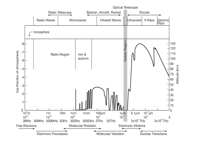
Figure 1: A plot of transmission through the atmosphere versus wavelength, $\lambda$ in metric units and frequency, $\nu$, in Hertz. The thick curve gives the fraction of the atmosphere (left vertical axis) and the altitude (right axis) needed to reach a transmission of 0.5. The fine scale variations in the thick curve are caused by molecular transitions (see Townes & Schawlow 1975). The thin vertical line on the left ($\sim 10$MHz) marks the boundary where ionospheric effects impede astronomical measurements. The labels above indicate the types of facilities needed to measure at the frequencies and wavelengths shown. For example, from the thick curve, at $\lambda$=100 $\mu$m, one half of the astronomical signal penetrates to an altitude of 45 km. In contrast, at $\lambda$=10 cm, all of this signal is present at the earth’s surface. The arrows at the bottom of the figure indicate the type of atomic or nuclear process that gives rise to the radiation at the frequencies and wavelengths shown above (from Wilson et al. 2008).

The broadband emission mechanism that dominates at meter wavelengths has been associated with the synchrotron process. Thus although the photons have energies in the micro electron volt range, this emission is caused by highly relativistic electrons (with $\gamma$ factors of more than 10³) moving in microgauss fields. In the centimeter and millimeter wavelength ranges, some broadband emission is produced by the synchrotron process, but additional emission arises from free-free Bremsstrahlung from ionized gas near high mass stars and quasi-thermal broadband emission from dust grains. In the mm/sub-mm range, emission from dust grains dominates, although free-free and synchrotron emission may also contribute. Spectral lines of molecules become more prominent at mm/sub-mm wavelengths (see Rybicki & Lightman 1979, Lequeux 2004, Tielens 2005).

Radio astronomy measurements are carried out at wavelengths vastly longer than those used in the optical range (see Fig. 1), so extinction of radio waves by dust is not an important effect. However, the longer wavelengths lead to lower angular resolution, $\theta$, since this is proportional to $\lambda$/D where D is the size of the aperture (see Jenkins & White 2001). In the 1940’s, the angular resolutions of radio telescopes were on scales of many arc minutes, at best. In time, interferometric techniques were applied to radio astronomy, following the method first used by Michelson. This was further developed, resulting in Aperture Synthesis, mainly by M. Ryle and associates at Cambridge University (for a history, see Kellermann & Moran 2001). Aperture synthesis has allowed imaging with angular resolutions finer than milli arc seconds with facilities such as the Very Long Baseline Array (VLBA).

Ground based measurements in the sub-mm wavelength range have been made possible by the erection of facilities on extreme sites such as Mauna Kea, the South Pole and the 5 km high site of the Atacama Large Millimeter/sub-mm Array (ALMA). Recently there has been renewed interest in high resolution imaging at meter wavelengths. This is due to the use of corrections for smearing by fluctuations in the electron content of the ionosphere and advances that facilitate imaging over wide angles (see, e.g., Venkata 2010). With time, the general trend has been toward higher sensitivity, shorter wavelength, and higher angular resolution.

Improvements in angular resolution have been accompanied by improvements in receiver sensitivity. Jansky used the highest quality receiver system then available. Reber had access to excellent systems. At the longest wavelengths, emission from astronomical sources dominates. At mm/sub-mm wavelengths, the transparency of the earth’s atmosphere is an important factor, adding both noise and attenuating the astronomical signal, so both lowering receiver noise and measuring from high, dry sites are important. At meter and cm wavelengths, the sky is more transparent and radio sources are weaker.

The history of radio astronomy is replete with major discoveries. The first was implicit in the data taken by Jansky. In this, the intensity of the extended radiation from the Milky Way exceeded that of the quiet Sun. This remarkable fact shows that radio and optical measurements sample fundamentally different phenomena. The radiation measured by Jansky was caused by the synchrotron mechanism; this interpretation was made more than 15 years later (see Rybicki & Lightman 1979). The next discovery, in the 1940’s, showed that the active Sun caused disturbances seen in radar receivers. In Australia, a unique instrument was used to associate this variable emission with sunspots (see Dulk 1985, Gary & Keller 2004). Among later discoveries have been: (1) discrete cosmic radio sources, at first, supernova remnants and radio galaxies (in 1948, see Kirshner 2004), (2) the 21 cm line of atomic hydrogen (in 1951, see Sparke & Gallagher 2007, Kalberla et al. 2005), (3) Quasi Stellar Objects (in 1963, see Begelman & Rees 2009), (4) the Cosmic Microwave Background (in 1965, see Silk 2008), (5) Interstellar molecules (see Herbst & Dishoeck 2009) and the connection with Star Formation, later including circumstellar and protoplanetary disks (in 1968, see Stahler & Palla 2005, Reipurth et al. 2007), (6) Pulsars (in 1968, see Lyne & Graham-Smith 2006), (7) distance determinations using source proper motions determined from Very Long Baseline Interferometry (see Reid 1993) and (8) molecules in high redshift sources (see Solomon & Vanden Bout 2005). These areas of research have led to investigations such as the dynamics of galaxies, dark matter, tests of general relativity, Black Holes, the early universe and gravitational radiation (for overviews see Longair 2006, Harwit 2006). Radio astronomy has been recognized by the physics community in that four Nobel Prizes (1974, 1978, 1993 and 2006) were awarded for work in this field. In chemistry, the community has been made aware of the importance of a more general chemistry involving ions and molecules (see Herbst 2001). Two Nobel Prizes for chemistry were awarded to persons actively engaged in molecular line astronomy.

Over time, the trend has been away from small groups of researchers constructing special purpose instruments toward the establishment of large facilities where users propose projects carried out by specialized staffs. These large facilities are in the process of becoming global. Similarly, the evolution of data reduction has been toward standardized packages developed by large teams. In addition, the demands of the interpretation of astronomical phenomena have led to multi-wavelength analyses interpreted with the use of detailed models.

Outside the norm are projects designed to measure a particular phenomenon. A prime example is the study of the cosmic microwave background (CMB) emission from the early universe. CMB data were taken with the COBE and WMAP satellites. These results showed that the CMB is is a Black Body (see Eq. 6) with a temperature of 2.73 K. Aside from a dipole moment caused by our motion, there is angular structure in the CMB at a very low level; this is being studied with the PLANCK satellite. Much effort continues to be devoted to measurements of the polarization of the CMB with ground-based experiments such as BICEP, CBI, DASI and QUIET. For details and references to other CMB experiments, see their websites. In spectroscopy, there have been extensive surveys of the 21 cm line of atomic hydrogen, H I (see Kalberla et al. 2005) and the rotational $J=1-0$ line from the ground state of carbon monoxide (see Dame et al. 1987). These surveys have been extended to external galaxies (see Giovanelli & Haynes 1991). During the Era of Reionization (redshift $z\sim$10 to 15), the H I line is shifted to meter wavelengths. The detection of such a feature is the goal of a number of individual groups, under the name HERA (Hydrogen Epoch of Reionization Arrays).

1.1 A Selected List of Radio Astronomy Facilities

There are a large number of existing facilities; a selection is listed here. General purpose instruments include the largest single dishes: the Parkes 64-m, the Robert C. Byrd Green Bank Telescope, hereafter GBT, the Effelsberg 100 meter, the 15-m James Clerk Maxwell Telescope (JCMT), the IRAM 30-m millimeter telescope and the 305-m Arecibo instrument. All of these have been in operation for a number of years. Interferometers form another category of instruments. The Expanded Very Large Array, the EVLA, is now in the test phase with ^′′shared risk^′′ observing. Other large interferometer systems are the VLBA, the Westerbork Synthesis Radio Telescope in the Netherlands, the Australia Telescope, the Giant Meter Wave Telescope in India, the MERLIN array a number of arrays at Cambridge University in the UK and the MOST facility in Australia. In the mm range, CARMA in California and Plateau de Bure in France are in full operation, as is the Sub-Millimeter Array of the Harvard-Smithsonian CfA and ASIAA on Mauna Kea, Hawaii. At longer wavelengths, the Low Frequency Array, LOFAR, has started the first measurements and will expand by adding stations throughout Europe. The Square Kilometer Array, the SKA, is in the planning phase as is the FASR solar facility, while the Australian SKA Precursor (ASKAP), the South African SKA precuror, (MeerKAT), the Murchison Widefield Array in Western Australia and Long Wavelength Array in New Mexico are under construction. A portion of the Allen Telescope Array, ATA, is in operation. A number of facilities are under construction, being commissioned or have recently become operational. At sub-mm wavelengths, the Herschel Satellite Observatory has been delivering data. The Five Hundred Meter Aperture Spherical Telescope, FAST, a design based on the Arecibo instrument, is being planned in China. This will be the world’s largest single aperture. The Large Millimeter Telescope, LMT, a joint Mexican-US project, will soon begin science operations as will the Stratospheric Far-Infrared Observatory (SOFIA) operated by NASA and the German DLR organization. Descriptions of these instruments are to be found in the internet. Finally, the most ambitious ground based astronomy project to date is ALMA which will start early science operations in late 2011 (for an account of the variety of ALMA science goals, see Bachiller & Cernicharo 2008).

2 Radiative Transfer and Black Body Radiation

The total flux of a source is obtained by integrating Intensity (in Watts m^-2 Hz^-1 steradian^-1) over the total solid angle $\Omega_{\rm s}$ subtended by the source

$$S_{\nu}=\int\limits_{\Omega_{\rm s}}I_{\nu}(\theta,\varphi)\cos\theta\,{\rm d}\Omega.$$ (1)

The flux density of astronomical sources is given in units of the Jansky (hereafter Jy), that is, $1\,{\rm Jy}=10^{-26}\,{\rm W\,m}^{-2}{\rm Hz}^{-1}$.

The equation of transfer is useful in interpreting the behavior of astronomcial sources, receiver systems, the effect of the earth’s atmosphere on measurements. Much of this analysis is based on a one dimensional version of the general expression as (see Lequeux 2004 or Tielens 2005):

$$\framebox{$\displaystyle\frac{{\rm d}I_{\nu}}{{\rm d}s}=-\kappa_{\nu}I_{\nu}+\varepsilon_{\nu}$}\quad.$$ (2)

The linear absorption coefficient $\kappa_{\nu}$ and the emissivity $\varepsilon_{\nu}$ are independent of the intensity $I_{\nu}$. From the optical depth definition ${\rm d}\tau_{\nu}=-\kappa_{\nu}\,{\rm d}s$, the Kirchhoff relation $\varepsilon_{\nu}/\kappa_{\nu}=B_{\nu}$ (see (Eq. 6)) and the assumption of an isothermal medium, the result is:

$$\framebox{$\displaystyle I_{\nu}(s)=I_{\nu}(0)\,{\rm e}^{-\tau_{\nu}(s)}+B_{\nu}(T)\,(1-\,{\rm e}^{-\tau_{\nu}(s)})$}\quad.$$ (3)

For a large optical depth, that is for $\tau_{\nu}(0)\rightarrow\infty$, (Eq. 3) approaches the limit

$$I_{\nu}=B_{\nu}(T)\thinspace.$$ (4)

This is case for planets and the 2.73  K CMB. From (Eq, 3), the difference between $I_{\nu}(s)$ and $I_{\nu}(0)$ gives

$$\Delta I_{\nu}(s)=I_{\nu}(s)-I_{\nu}(0)=(B_{\nu}(T)-I_{\nu}(0))(1-{\rm\,e}^{-\tau})\;.$$ (5)

this represents the result of an on-source minus off-source measurement, which is relevant for discrete sources.

The spectral distribution of the radiation of a black body in thermodynamic equilibrium is given by the Planck law

$$\framebox{$\displaystyle B_{\nu}(T)=\frac{2h\nu^{3}}{c^{2}}\frac{1}{{\rm e}^{h\nu/kT}-1}$}\quad.$$ (6)

If $h\nu\ll kT$, the Rayleigh-Jeans Law is obtained:

$$\framebox{$\displaystyle B_{\rm RJ}(\nu,T)=\frac{2\nu^{2}}{c^{2}}kT$}\quad.$$ (7)

In the Rayleigh-Jeans relation, the brightness and the thermodynamic temperatures of Black Body emitters are strictly proportional (Eq. 7). This feature is useful, so the normal expression of brightness of an extended source is brightness temperature $T_{\rm B}$:

$$T_{\rm B}=\frac{c^{2}}{2k}\frac{1}{\nu^{2}}\,I_{\nu}=\frac{\lambda^{2}}{2k}\,I_{\nu}\thinspace.$$ (8)

If $I_{\nu}$ is emitted by a black body and $h\nu\ll kT$ then (Eq. 8) gives the thermodynamic temperature of the source, a value that is independent of $\nu$. If other processes are responsible for the emission of the radiation (e.g., synchrotron, free-free or broadband dust emission), $T_{\rm B}$ will depend on the frequency; however (Eq. 8) is still used. If the condition $\nu(\rm GHz)\ll 20.84\left(T(\rm K)\right)$ is not valid, (Eq. 8) can still be applied, but $T_{\rm B}$ will differ from the thermodynamic temperature of a black body. However, corrections are simple to obtain.

If (Eq. 8) is combined with (Eq. 5), the result is an expression for brightness temperature:

$$J(T)=\frac{c^{2}}{2k\nu^{2}}(B_{\nu}(T)-I_{\nu}(0))(1-{\rm\,e}^{-\tau_{\nu}(s)})\;.$$

The expression $J(T)$ can be expressed as a temperature in most cases. This quantity is referred to as $T^{*}_{\rm R}$, the radiation temperature in the mm/sub-mm range, or the brightness temperature, $T_{\rm B}$ for longer wavelengths. In the Rayleigh-Jeans approximation the equation of transfer is:

$$\framebox{$\displaystyle\frac{{\rm d}T_{\rm B}(s)}{{\rm d}\tau_{\nu}}=T_{\rm bk}(0)-T(s)$}\quad,$$ (9)

where $T_{\rm B}$ is the measured quantity, $T_{\rm bk}(s)$ is the background source temperature and $T(s)$ is the temperature of the intervening medium If the medium is isothermal, the general (one dimensional) solution becomes

$$\framebox{$\displaystyle T_{\rm B}=T_{\rm bk}(0)\,{\rm e}^{-\tau_{\nu}(s)}+T\,(1-\,{\rm e}^{-\tau_{\nu}(s)})$}\quad.$$ (10)

2.1 The Nyquist Theorem and Noise Temperature

This theorem relates the thermodynamic quantity temperature to the electrical quantities voltage and power. This is essential for the analysis of noise in receiver systems. The average power per unit bandwidth, $P_{\nu}$ (also referred to as Power Spectral Density, PSD), produced by a resistor $R$ is

$$P_{\nu}=\langle iv\rangle=\frac{\langle v^{2}\rangle}{2R}=\frac{1}{4R}\langle v_{\rm N}^{2}\rangle\thinspace,$$ (11)

where $v(t)$ is the voltage that is produced by $i$ across $R$, and $\langle\cdots\rangle$ indicates a time average. The first factor $\frac{1}{2}$ arises from the condition for the transfer of maximum power from $R$ over a broad range of frequencies. The second factor $\frac{1}{2}$ arises from the time average of $v^{2}$. Then

$$\langle v_{\rm N}^{2}\rangle=4R\,k\,T\;.$$ (12)

When inserted into (Eq. 11), the result is

$$P_{\nu}=k\,T\;.$$ (13)

(Eq. 13) can also be obtained by a reformulation of the Planck law for one dimension in the Rayleigh-Jeans limit. Thus, the available noise power of a resistor is proportional to its temperature, the noise temperature $T_{\rm N}$, independent of the value of $R$ and of frequency.

Not all circuit elements can be characterized by thermal noise. For example a microwave oscillator can deliver 1 $\mu$W, the equivalent of more than $10^{16}$ K, although the physical temperature is $\sim$300 K. This is an example of a very nonthermal process, so temperature is not a useful concept in this case.

2.2 Overview of Intensity, Flux Density and Main Beam Brightness Temperature

Temperatures in radio astronomy have given rise to some confusion. A short summary with references to later sections is given here. Power is measured by an instrument consisting of an antenna and receiver. The power input can be calibrated and expressed as Flux Density or Intensity. For very extended sources, Intensity (see (Eq. 8)) can be expressed as a temperature, the main beam brightness temperature, T_MB. To obtain T_MB, the measurements must be calibrated (Section 5.3) and corrected using the appropriate efficiencies (see Eq. 37 and following). For discrete sources, the combination of (Eq. 1) with (Eq. 8) gives:

$$\framebox{$\displaystyle S_{\nu}=\frac{2\,k\,\nu^{2}}{c^{2}}T_{\rm B}\,\mbox{\greeksym{D}}\Omega$}\quad.$$ (14)

For a source with a Gaussian spatial distribution, this relation is

$$\left[\frac{S_{\nu}}{\rm Jy}\right]=0.0736\,T_{\rm B}\,\left[\frac{\theta}{\rm arc\,seconds}\right]^{2}\left[\frac{\lambda}{\rm mm}\right]^{-2}$$ (15)

if the flux density $S_{\nu}$ and the actual (or ^′′true^′′) source size are known, then the true brightness temperature, $T_{\rm B}$, of the source can be determined. For Local Thermodynamic Equilibrium (LTE), $T_{\rm B}$ represents the physical temperature of the source. If the apparent source size, that is, the source angular size as measured with an antenna is known, (Eq. 15) allows a calculation of T_MB. For discrete sources, T_MB depends on the angular resolution. If the antenna beam size (see Fig. 3 and discussion) has a Gaussian shape $\theta_{\rm b}$, the relation of actual $\theta_{\rm s}$ and apparent size $\theta_{\rm o}$ is:

$$\theta_{\rm o}^{2}=\theta_{\rm s}^{2}+\theta_{\rm b}^{2}\,.$$ (16)

then from (Eq. 14), the relation of T_MB and T_B is:

$$T_{\rm MB}\left(\theta_{\rm s}^{2}+\theta_{\rm b}^{2}\right)=T_{\rm B}\,\theta_{\rm s}^{2}$$ (17)

Finally, the PSD entering the receiver (Eq. 13) is antenna temperature, T_A; this is relevant for estimating signal to noise ratios (see (Eq. 39) and (Eq. 42)). To establish temperature scales and relate received power to source parameters for filled apertures, see Section 5.3. For interferometry and Aperture Synthesis, see Section 6.

2.3 Interstellar Dispersion and Polarization

Pulsars emit radiation in a short time interval (see Lorimer & Kramer 2004, Lyne & Graham-Smith 2006). If all frequencies are emitted at the same instant, the arrival time delay of different frequencies is caused by the ionized Interstellar Medium (ISM). This is characterized by the quantity $\int_{0}^{L}N(l){\rm\,d}l$, which is the column density of the electrons to a distance $L$. Since distances in astronomy are measured in parsecs it has become customary to express the dispersion measure as:

$${\mathrm{DM}}=\int\limits_{0}^{L}\left(\frac{N}{\mathrm{cm}^{-3}}\right){\rm\,d}\left({\frac{l}{\mathrm{pc}}}\right)$$ (18)

The lower frequencies are delayed more in the ISM, so the relative time delay is:

$$\frac{\Delta\tau_{\mathrm{D}}}{\mbox{\greeksym{m}}\rm s}=1.34\times 10^{-9}\left[\frac{\mathrm{DM}}{\mathrm{cm}^{-2}}\right]\left[\displaystyle\frac{1}{\left(\displaystyle\frac{\nu_{1}}{\mathrm{MHz}}\right)^{2}}-\frac{1}{\left(\displaystyle\frac{\nu_{2}}{\mathrm{MHz}}\right)^{2}}\right]$$ (19)

Since both time delay $\Delta\tau_{\mathrm{D}}$ and observing frequencies $\nu_{1}<\nu_{2}$ can be measured with high precision, a very accurate value of DM for a given pulsar can be determined. Provided the distance to the pulsar, $L$, is known, a good estimate of the average electron density between observer and pulsar can be found. However since $L$ is usually known with moderate accuracy, only approximate values for $N$ can be obtained. Often the opposite procedure is used: From reasonable values for $N$, a measured DM provides information on the unknown distance $L$ to the pulsar.

Broadband linear polarization is caused by non-thermal processes (see Rybicki & Lightman 1979) including Pulsar radiation, quasi-thermal emission from aligned, non-spherical dust grains (see Hildebrand 1983) and scattering from free electrons. Faraday rotation will change the position angle of linear polarization as the radiation passes through an ionized medium; this varies as $\lambda^{2}$, so this effect is larger for longer wavelengths. It is usual to characterize polarization by the four Stokes Parameters, which are the sum or difference of measured quantities. The total intensity of a wave is given by the parameter $I$. The amount and angle of linear polarization by the parameters $Q$ and $U$, while the amount and sense of circular polarization is given by the parameter $V$. Hertz dipoles are sensitive to a single linear polarization. By rotating the dipole over an angle perpendicular to the direction of the radiation, it is possible to determine the amount and angle of linearly polarized radiation. Helical antennas or arrangements of two Hertz dipoles are sensitive to circular polarization. Generally, polarized radiation is a combination of linear and circular, and is usually less than 100% polarized, so four Stokes parameters must be specified. The definition of the sense of circular polarization in radio astronomy is the same as in Electrical Engineering but opposite to that used in the optical range; see Born & Wolf (1965) for a complete analysis of polarization, using the optical definition of circular polarization. Poincaré introduced a representation that permits an easy visualization of all the different states of polarization of a vector wave. See Thompson et al. (2001), Crutcher (2008), Thum et al. (2008) or Wilson et al. (2008) for more details.

3 Receiver Systems

3.1 Coherent and Incoherent Receivers

Receivers are assumed to be linear power measuring devices, i. e. any non-linearity is a small quantity. There are two types of receivers: coherent and incoherent. Coherent receivers are those which preserve the phase of the input radiation while incoherent do not. Heterodyne (technically ^′′superheterodyne^′′) receivers are those which those which shift the frequency of the input but preserve phase. The most commonly used coherent receivers employ heterodyning, that is, frequency shifting (see Section 4.2.1). The most commonly used incoherent receivers are bolometers (Section 4.1); these are direct detection receivers, that is, operate at sky frequency. Both coherent and incoherent receivers add noise to the astronomical input signal; it is assumed that the noise of both the input signal and the receiver follow Gaussian distributions. The noise contribution of coherent receivers is expressed in Kelvins. Bolometer noise is characterized by the Noise Equivalent Power, or NEP, in units of Watts Hz^-1/2 (see Section 3.1.1 and Section 5.3.3). NEP is the input power level which doubles the output power. More extensive discussions of receiver properties are given in Rieke (2002) or Wilson et al. (2008).

To analyze the performance of a receiver, the commonly accepted model is an ideal receiver with no internal noise, but connected to two noise sources, one for the external noise (including the astronomical signal) and a second for the receiver noise. To be useful, receiver systems must increase the input power level. The noise contribution is characterized by the Noise Factor, $F$. If the signal-to-noise ratio at the input is expressed as $(S_{1}/N_{1})$ and at the output as $(S_{2}/N_{2})$, the noise factor is:

$$F=\frac{S_{1}/N_{1}}{S_{2}/N_{2}}\;.$$ (20)

A further step is to assume that the signal is amplified by a gain factor $G$ but otherwise unchanged. Then $S_{2}=G\,S_{1}$ and:

$$F=\frac{N_{2}}{G\,N_{1}}\;.$$ (21)

For a direct detection system such as a bolometer, $G=1$. For coherent receivers, there must be a minimum noise contribution (see Section 4.2.4), so $F>1$. For coherent receivers $F$ is expressed in temperature units as $T_{R}$ using the relation

$$T_{R}=(F-1)\cdot 290{\rm K}\;.$$ (22)

3.1.1 Receiver Calibration

Heterodyne receiver noise performance is usually expressed in degrees Kelvin. In the calibration process, a power scale (the PSD) is established at the receiver input. This is measured in terms of the noise temperature. To calibrate a receiver, the noise temperature increment $\Delta T$ at the receiver input must be related to a given measured receiver output increment $\Delta z$ (this applies to coherent receivers which have a wide dynamic range and a total power or ^′′DC^′′ response). Usually resistive loads at two known (thermodynamic) temperatures $T_{\rm L}$ and $T_{\rm H}$ are used. The receiver outputs are $z_{\rm L}$ and $z_{\rm H}$, while $T_{\rm L}$ and $T_{\rm H}$ are the resistive loads at two temperatures. The relations are:

$$z_{\rm L} = (T_{\rm L}+T_{\rm R})\,G\thinspace,$$

$$z_{\rm H} = (T_{\rm H}+T_{\rm R})\,G\thinspace,$$

taking

$$y=z_{\rm H}/z_{\rm L}\thinspace.$$ (23)

the result is:

$$\framebox{$\displaystyle T_{\rm rx}=\frac{T_{\rm H}-T_{\rm L}\,y}{y-1}$}\quad,$$ (24)

This is known as the ^′′y-factor^′′; the procedure is a ^′′hot-cold^′′ measurement. The determination of the y factor is calculated in the Rayleigh-Jeans limit. Absorbers at temperatures of $T_{\rm H}$ and $T_{\rm L}$ are used to produce the inputs. Often these are chosen to be at the ambient temperature ($T_{\rm H}\cong 293$ K or $20\hbox{${}^{\circ}$}$ C) and at the temperature of liquid nitrogen ($T_{\rm L}\cong 78$ K or $-195\hbox{${}^{\circ}$}$ C). When receivers are installed on antennas, such ^′′hot-cold^′′ calibrations are done only infrequently. As will be discussed in Section 5.3.2, in the cm and meter range, calibration signals are provided by noise diodes; from measurements of sources with known flux densities intensity scales are established. Any atmospheric corrections are assumed to be small at these wavelengths. As will be discussed in Section 5.3.3, in the mm/sub-mm wavelength range, from measurements of an ambient load (or two loads at different temperatures), combined with measurements of emission from the atmosphere and models of the atmosphere, estimates of atmospheric transmission are made.

Bolometer performance is characterized by the Noise Equivalent Power, or NEP, given in units of Watts Hz^-1/2. The expression for NEP can be related to a receiver noise temperature. For ground based bolometer systems, background noise dominates. For these, the background noise is given as T_BG:

$$\framebox{$\displaystyle{\rm NEP}=2\varepsilon\,k\,T_{\rm BG}\,\sqrt{\Delta\nu}$}\quad.$$ (25)

here $\varepsilon$ is the emissivity of the background and $\Delta\nu$ is the bandwidth. Typical values for ground-based mm/sub-mm bolometers are $\varepsilon=0.5$, T${}_{\rm BG}=300$ K and $\Delta\nu=100$ GHz. For these values, NEP$=1.3\times 10^{-15}$   Watts Hz^-1/2. With the collecting area of the IRAM 30 m or the JCMT telescopes, sources in the milli-Jansky (mJy) range can be measured.

Usually bolometers are ^′′A. C.^′′ coupled, that is, the output responds to differences in the input power, so hot-cold measurements are not useful for characterizing bolometers. The response of bolometers is usually determined by measurements of sources with known flux densities, followed by measurements at, for example, elevations of 20^o, 30^o, 60^o and 90^o to determine the atmospheric transmission (see Section 5.3.4).

3.1.2 Noise Uncertainties due to Random Processes

The noise contributions from source, atmosphere, ground, telescope surface and receiver are always additive:

$$T_{\rm sys}=\sum T_{i}$$ (26)

From Gaussian statistics, the Root Mean Square, RMS, noise is given by the mean value divided by the square root of the number of samples. From the estimate that the number of samples is given by the product of receiver bandwidth multiplied by the integration time, the result is:

$$\framebox{$\displaystyle\mbox{\greeksym{D}}T_{\rm RMS}=\frac{T_{\rm sys}}{\displaystyle\sqrt{\mbox{\greeksym{D}}\nu\,\tau}}$}\quad.$$ (27)

A much more elaborate derivation is to be found in Chapter 4 of Rohlfs & Wilson (2004), while a somewhat simpler account is in Wilson et al. (2008). The calibration process in (Section 3.1.1) allows the receiver noise to be expressed in degrees Kelvin. The relation of T_sys to T_rx is $T_{\rm sys}=T_{\rm A}+T_{\rm rx}$, where $T_{\rm A}$ represents the power entering the receiver; at some wavelengths $T_{\rm A}$ will dominate $T_{\rm rx}$. In the mm/sub-mm range, use is made of T${}_{\rm sys}^{*}$, the system noise outside the atmosphere, since the attenuation of astronomical radiation is large. This will be presented in Section 5.3.1 and following.

3.1.3 Receiver Stability

Sensitive receivers are designed to achieve a low value for $T_{\rm rx}$. Since the signals received are of exceedingly low power, receivers must also provide large receiver gains, $G$ (of order $10^{12}$), for sufficient output power. Thus even very small gain instabilities can dominate the thermal receiver noise. Since receiver stability considerations are of prime importance, comparison switching was necessary for early receivers (Dicke 1946). Great advances have been made in improving receiver stability since the 1960’s so the need for rapid switching is lessened. In the meter and cm wavelength range, the time between reference measurements has increased. However in the mm/sub-mm range, instabilities of the atmosphere play an important role; to insure that noise decreases following (Eq. 27), the effects of atmospheric and/or receiver instabilities must be eliminated. For single dish measurements, atmospheric changes can be compensated for by rapidly differencing a measurement of the target source and a reference. Such comparison or ^′′Dicke^′′ switched measurements are necessary for ground-based observations. If a typical procedure consists of using a total power receiver to measure on-source for 1/2 of the total time, then an off-source comparison for 1/2 of the time and taking the difference of on-source minus off-source measurements, the $\mbox{\greeksym{D}}T_{\rm RMS}$ will be a factor of 2 larger than the value given by (Eq. 27).

4 Practical Aspects of Receivers

This section concentrates on receivers that are currently in use. For more details see Goldsmith (1988), Rieke (2002), or Wilson et al. (2008).

4.1 Bolometer Radiometers

Bolometers operate by use of the effect that the resistance, $R$, of a material varies with the temperature. In the 1970’s, the most sensitive bolometers were semiconductor devices pioneered by F. Low. This is achieved when the bolometer element is cooled to very low temperatures. When radiation is incident, the characteristics change, so this is a measure of the intensity of the incident radiation. Because this is a thermal effect, it is independent of the frequency and polarization of the radiation absorbed. Thus bolometers are intrinsically broadband devices. It is possible to mount a polarization-sensitive device before the bolometer and thereby measure the direction and degree of linear polarization. Also, it is possible to carry out spectroscopy, if frequency sensitive elements, either filters, Michelson or Fabry-Perot interferometers, are placed before the bolometer element. Since these spectrometers operate at the sky frequency, the fractional resolution ($\mbox{\greeksym{D}}\nu/\nu$) is at best $\sim 10^{-4}$. The data from each bolometer detector element (pixel) must be read out and then amplified.

For single dish (i. e. filled apertures) broadband continuum measurements at $\lambda<$ 2 mm, multi-beam bolometers are the most common systems and such systems can have a large number of beams. A promising new development in bolometer receivers is Transition Edge Sensors referred to as TES bolometers. These superconducting devices may allow more than an order of magnitude increase in sensitivity, if the bolometer is not background limited. For bolometers used on earth-bound telescopes, the improvement with TES systems may be only $\sim$2–3 times more sensitive than the semiconductor bolometers, but TES’s will allow readouts from a much larger number of pixels.

A number of large bolometer arrays have produced numerous publications: (1) MAMBO2 (MAx-Planck-Millimeter Bolometer) used on the IRAM 30-m telescope at 1.3 mm, (2) SCUBA (Submillimeter Common User Bolometer Array; Holland et al. 1999) on the JCMT, (3) the LABOCA (LArge Bolometer CAmera) array on the APEX 12 meter telescope, (4) SHARC (Sub-mm High Angular Resolution Camera) on the Caltech Sub-mm Observatory 10-m telescope and (5) MUSTANG (MUtiplexed Squid TES Array) on the GBT. SCUBA will be replaced with SCUBA-2 now being constructed at the U. K. Astronomy Technology Center, and there are plans to replace the MUSTANG array by MUSTANG-2, which is a larger TES system.

4.2 Coherent Receivers

Usually, coherent receivers make use of heterodyning to shift the signal input frequency without changing other properties of the input signal; in practice, this is carried out by the use of mixers (Section 4.2.2). The heterodyne process is used in all branches of communications technology; use of heterodyning allows measurements with unlimited spectral resolution. Although heterodyne receivers have a number of components, these systems have more flexibility than bolometers.

4.2.1 Noise Contributions in Coherent Receivers

The noise generated in the first element dominates the system noise. The mathematical expression is given by the Friis relation which accounts for the effect of cascaded amplifiers on the noise performance of a receiver:

$$\framebox{$\displaystyle T_{\rm S}=T_{\rm S1}+\frac{1}{G_{1}}T_{\rm S2}+\frac{1}{G_{1}G_{2}}T_{\rm S3}+\dots+\frac{1}{G_{1}G_{2}\dots G_{n-1}}T_{{\rm S}n}$}\quad.$$ (28)

Where $G_{1}$ is the gain of the first element, and $T_{\rm S1}$ is the noise temperature of this element. For $\lambda>$3 mm ($\nu<115$GHz), the best cooled first elements, High Electron Mobility Transistors (HEMTs), typically have $G_{1}=10^{3}$ and $T_{\rm S1}=50$K; for $\lambda<$0.8 mm, the best cooled first elements, superconducting mixers, typically have $G_{1}\leq 1$, that is, a small loss, and $T_{\rm S1}\leq 500$K. The stage following the mixer should have the lowest noise temperature and high gain.

4.2.2 Mixers

Mixers have been used in heterodyne receivers since Jansky’s time. At first these were metal-oxide-semiconductor or Schottky mixers. Mixers allow the signal frequency to be changed without altering the characteristics of the signal. In the mixing process, the input signal is multiplied by an intense monochromatic signal from a local oscillator, LO. The frequency stability of the LO signal is maintained by a stabilization device in which the LO signal is compared with a stable input, in recent times, an atomic standard. These phaselock loop systems produce a pure, highly stable, monochromatic signal. The mixer can be operated in the Double Sideband (DSB) mode, in which two sky frequencies, ^′′signal^′′ and ^′′image^′′ at equal separations from the LO frequency (equal to the IF frequency) are shifted into intermediate (IF) frequency band. For spectral line measurements, usually one sideband is wanted, but the other not. DSB operation adds both noise and (usually) unwanted spectral lines; for spectral line measurements, single sideband (SSB) operation is preferred. In SSB operation, the unwanted sideband is suppressed, at the cost of more complexity. In the sub-mm wavelength ranges, DSB mixers are still commonly used as the first stage of a receiver; in the mm and cm ranges, SSB operation is now the rule.

A significant improvement can be obtained if the mixer junction is operated in the superconducting mode. The noise temperatures and LO power requirements of superconducting mixers are much lower than Schottky mixers. Finally, the physical layout of such devices is simpler since the mixer is a planar device, deposited on a substrate by lithographic techniques. SIS mixers consist of a superconducting layer, a thin insulating layer and another superconducting layer (see Phillips & Woody 1982).

Figure 2: Receiver noise temperatures for coherent amplifier systems compared to the temperatures from the Milky Way galaxy (at long wavelengths, on left part of figure) and the atmosphere (at mm/sub-mm wavelengths on the right side). The atmospheric emission is based on a model of zenith emission for 0.4 mm of water vapor, that is, excellent weather (plot from B. Nicolic (Cambridge Univ.) using the ^′′AM^′′ program of S. Paine (Harvard-Smithsonian Center for Astrophysics)). This does not take into account the absorption of the astronomical signal. In the 1 to 26 GHz range, the two horizontal lines represent the noise temperatures of the best HEMT amplifiers, while the solid line represents the noise temperatures of maser receivers. The shaded region between 85 and 115.6 GHz is the receiver noise for the SEQUOIA array (Five College Radio Astronomy Observatory) which consists of monolithic millimeter integrated circuits (MMIC). The meaning of the other symbols is given in the upper left of the diagram (SIS’s are Superconductor-Insulator-Superconductor mixers, HEB’s are Hot Electron Bolometer mixers). The double sideband (DSB) mixer noise temperatures were converted to single sideband (SSB) noise temperatures by doubling the receiver noise. The ALMA mixer noise temperatures are SSB, as are the HEMT values. The line marked ^′′10 h$\nu$/kT^′′ refers to the limit described in (Eq. 30). Some data used in this diagram are taken from Rieke (2002). The figure is from Wilson et al. (2008)

Superconducting Hot Electron Bolometer-mixers (HEB) are heterodyne devices, in spite of the name. These mixers make use of superconducting thin films which have sub-micron sizes (see Kawamura et al. 2002).

A number of multi-beam heterodyne cameras are in operation in the cm range, but only a few in the mm/sub-mm range. The first mm multi-beam system was the SEQUOIA array receiver pioneered by S. Weinreb; such devices are becoming more common. In contrast, multibeam systems that use SIS front ends are rare. Examples are a 9 beam Heterodyne Receiver Array of SIS mixers at 1.3 mm, HERA, on the IRAM 30-m millimeter telescope, HARP-B, a 16 beam SIS system in operation at the JCMT for 0.8 mm and the CHAMP+ receiver at the Max-Planck-Inst. für Radioastronomy on the APEX 12-m telescope.

4.2.3 Square Law Detectors

For heterodyne receivers the input is normally amplified (for $\nu<115$GHz), translated in frequency and then detected in a device that produces an output signal $y(t)$ which is proportional to the square of $v(t)$:

$$y(t)=a\,v^{2}(t)$$ (29)

Once detected, phase information is lost. For interferometers, the output of each antenna is a voltage, shifted in frequency and then digitized. This output is brought to a central location for correlation.

4.2.4 The Minimum Noise in a Coherent System

The ultimate limit for coherent receivers or amplifiers is obtained by an application of the Heisenberg uncertainty principle involving phase and number of photons. From this, the $minimum$ noise of a coherent amplifier results in a receiver noise temperature of

$$\framebox{$\displaystyle T_{\rm rx}({\rm minimum})=\frac{h\nu}{k}$}\quad.$$ (30)

For incoherent detectors, such as bolometers, phase is not preserved, so this limit does not exist. In the mm wavelength region, this noise temperature limit is quite small; at $\lambda$=2.6 mm ($\nu$=115 GHz), this limit is 5.5 K. The value for the ALMA receiver in this range is about 5 to 6 times the minimum. A significant difference between radio and optical regimes is that the minimum noise in the radio range is small, so that the power from a single receiver can be amplified and then divided. For example, for the EVLA, the voltage output of all 351 antenna pairs are combined with little or no loss in the signal-to-noise ratio. Another example is given in Section 4.3.1, where a radio polarimeter can produce all four Stokes parameters from two inputs without a loss of the signal-to-noise ratio.

4.3 Back Ends: Polarimeters & Spectrometers

The term ^′′Back End^′′ is used to specify the devices following the IF amplifiers. Many different back ends have been designed for specialized purposes such as continuum, spectral or polarization measurements.

For a single dish continuum correlation receiver, the (identical) receiver input is divided, amplified in two identical systems and then the outputs are multiplied. The gain fluctuations are uncorrelated but the signals are, so the effect on the output is the same as with a Dicke switched system, but with no time spent on a reference.

4.3.1 Polarimeters

A typical heterodyne dual polarization receiver consists of two identical systems, each sensitive to one of the two orthogonal polarizations, linear or circular. Both systems must be connected to the same local oscillator to insure that the phases have a definite relation. Given this arrangement, a polarimeter can provide values of all four Stokes parameters simultaneously. All Stokes parameters can also be measured using a single receiver whose input is switched from one sense of polarization to the other, but then the integration time for each polarization will be halved.

4.3.2 Spectrometers

Spectrometers analyze the spectral information contained in the radiation field. To accomplish this, the spectrometer must be SSB and the frequency resolution $\Delta\nu$ is usually very good, sometimes in the kHz range. In addition, the time stability must be high. If a resolution of $\Delta\nu$ is to be achieved for the spectrometer, all those parts of the system that enter critically into the frequency response have to be maintained to better than $0.1\,\Delta\nu$. For an overview of the current state of spectrometers, see Baker et al. (2007).

Conceptually, the simplest spectrometer is composed of a set of $n$ adjacent filters, each with a bandwidth $\Delta\nu$. Following each filter is a square-law detector and integrator. For a finer resolution, another set of $n$ filters must be constructed.

Another approach to spectral analysis is to Fourier Transform (FT) the input, $v(t)$, to obtain $v(\nu)$ and then square $v(\nu)$ to obtain the Power Spectral Density. The maximum bandwidth is limited by the sampling rate. From (another!) Nyquist theorem, it is necessary to sample at a rate equal to twice the bandwidth. In the simplest scheme, for a bandwidth of 1 GHz, the sampling must occur at a rate of 2 GHz. After sampling and Fourier Transform, the output is squared to produce power in an ^′′FX^′′ autocorrelator. For $10^{3}$ samples, each channel will have a 1 MHz resolution.

For ^′′XF^′′ systems, the input $v(t)$ is multiplied (the ^′′X^′′) with a delayed signal $v(t-\tau)$ to obtain the autocorrelation function $R(\tau)$. This is then Fourier Transformed to obtain the spectrum. For $10^{3}$ samples, there will be $10^{3}$ frequency channels. For an XF system the time delays are performed in a set of serial digital shift registers with a sample delayed by a time $\tau$. Autocorrelation can also be carried out with the help of analog devices using a series of cable delay lines; these can provide very large bandwidths. The first XF system for astronomy was a digital autocorrelator built by S. Weinreb in 1963.

The two significant advantages of digital spectrometers are: (1) flexibility and (2) a noise behavior that follows $1/\sqrt{t}$ after many hours of integration. The flexibility allows the choice of many different frequency resolutions and bandwidths or even to employ a number of different spectrometers, each with different bandwidths, simultaneously.

A serious drawback of digital auto and cross correlation spectrometers had been limited bandwidths. However, advances in digital technology in recent years have allowed the construction of autocorrelation spectrometers with several 10³ channels covering instantaneous bandwidths of several GHz.

Autocorrelation systems are used in single antennas. The calculation of spectra makes use of the symmetric nature of the autocorrelation function, ACF, so the number of delays gives the number of spectral channels.

Cross-correlators are used in interferometers and in some single dish applications. When used in an interferometer, the cross-correlation is between different inputs so will not necessarily be symmetric. Thus, the zero delay of the cross-correlator is placed in channel $N/2$. The number of delays, $N$, allows the determination of $N/2$ spectral intensities, and $N/2$ phases. The cross-correlation hardware can employ either an XF or a FX correlator. For more details about the use of cross-correlation, see Section 6.

Until recently, spectrometers with bandwidths of several GHz often made use of Acoustic Optical analog techniques. The Acoustic Optical Spectrometer (AOS) makes use of the diffraction of light by ultrasonic waves: these cause periodic density variations in the crystal through which it passes. These density variations in turn cause variations in the bulk constants of the crystal, so that a plane light wave passing through this medium will be modulated by the interaction with the crystal. The modulated light is detected in a charge coupled device. Typical AOS’s have an instantaneous bandwidth of 2 GHz and 2000 spectral channels.

In all cases, the spectra of the individual channels of a spectrometer are expressed in terms of temperature with the relation:

$$T_{i}=\left[\left(S_{i}-R_{i}\right)/R_{i}\right]\cdot T_{\rm sys}$$ (31)

where $S_{i}$ is the normalized spectrum of channel $i$ for the on-source measurement and $R_{i}$ is the corresponding reference for this channel. For mm/sub-mm spectra, $T_{\rm sys}$ is replaced by $T_{\rm sys}^{*}$ (corrected for atmospheric losses; see Section 5.3.3). For cross-correlators, as used in interferometers, the signals from two antennas are multiplied. In this case, the value of $T_{\rm sys}$ is the square root of the product of the system noise temperatures of the two systems.

5 Antennas

The antenna serves to focus power into the feed, a device that efficiently transfers power in the electromagnetic wave to the receiver. According to the principle of reciprocity, the properties of antennas such as beam sizes, efficiencies etc. are the same whether these are used for receiving or transmitting. Reciprocity holds in astronomy, so it is usual to interchangeably use expressions that involve either transmission or reception when discussing antenna properties. All of the following applies to the far-field radiation.

5.1 The Hertz Dipole

The total power radiated from a Hertz dipole carrying an oscillating current $I$ at a wavelength $\lambda$ is

$$\framebox{$\displaystyle P=\frac{2c}{3}\left(\frac{I\Delta l}{2\lambda}\right)^{2}$}\quad.$$ (32)

For the Hertz dipole, the radiation is linearly polarized with the electric field along the direction of the dipole. The radiation pattern has a donut shape, with the cylindrically symmetric maximum perpendicular to the axis of the dipole. Along the direction of the dipole, the radiation field is zero. To improve directivity, reflecting screens have been placed behind a dipole, and in addition, collections of dipoles, driven in phase, are used. Hertz dipole radiators have the best efficiency when the size of the dipole is $1/2\,\lambda$ .

5.2 Filled Apertures

This Section is a simplified description of antenna properties needed for the interpretation of astronomical measurements. For more detail, see Baars (2007). At cm and shorter wavelengths, flared waveguides (^′′feed horns^′′) or dipoles are used to convey power focussed by the antenna (i. e., electromagnetic waves in free space) to the receiver (voltage). At the longest wavelengths, dipoles are used as the antennas. Details are to be found in Love (1976) and Goldsmith (1988, 1994).

5.2.1 Angular Resolution and Efficiencies

From diffraction theory (see Jenkins & White 2001), the angular resolution of a reflector of diameter $D$ at a wavelength $\lambda$ is

$$\framebox{$\displaystyle\theta=k\frac{\lambda}{D}$}\quad.$$ (33)

where $k$ is of order unity. This universal result gives a value for $\theta$ (here in radians when $D$ and $\lambda$ have the same units). Diffraction theory also predicts the unavoidable presence of sidelobes, i. e. secondary maxima. The sidelobes can be reduced by tapering the antenna illumination. Tapering lowers the response to very compact sources and increases the value of $\theta$, i. e. widens the beam.

The reciprocity concept provides a method to measure the power pattern (response pattern or Point Spread Function, PSF) using transmitters. However, the distance from a large antenna A (diameter $D\gg\lambda$) to a transmitter B (small in size) must be so large that B produces plane waves across the aperture $D$ of antenna A, that is, so B is in the far field of A. This is the Rayleigh distance; it requires that the curvature of a wavefront emitted by B is much less than $\lambda$/16 across the geometric dimensions of antenna A. By definition, at the Rayleigh distance $\mathcal{D}$, the curvature must be $\gg D^{2}/8\lambda$ for an antenna of diameter $D$.

Often, the normalized power pattern is measured:

$$\framebox{$\displaystyle P_{\rm n}(\vartheta,\varphi)=\frac{1}{P_{\rm max}}\,P(\vartheta,\varphi)$}\quad.$$ (34)

For larger apertures, the transmitter is usually replaced by a small diameter radio source of known flux density (see Baars et al. 1977, Ott et al. 1994). The flux densities of a few primary calibration sources are determined by measurements using horn antennas at centimeter and millimeter wavelengths. At mm/sub-mm wavelengths, it is usual to employ planets, or moons of planets, whose surface temperatures are known (see Altenhoff 1985, Sandell 1994).

[width=2.6cm,height=5.9cm]wilson-fig3.pdf

Figure 3: A polar power pattern showing the main beam, and near and far sidelobes. The weaker far sidelobes have been combined to form the stray pattern

The beam solid angle $\Omega_{\rm A}$ of an antenna is given by

$$\framebox{$\displaystyle\Omega_{\rm A}=\parbox{22.76219pt}{$\vspace*{-2mm}{\displaystyle\int\!\!\int\atop{\!\!\!\!\!\scriptstyle 4\pi}}$ }P_{\rm n}(\vartheta,\varphi)\,{\rm\,d}\Omega=\int\limits_{0}^{2\pi}\!\int\limits_{0}^{\pi}P_{\rm n}(\vartheta,\varphi)\sin\vartheta{\rm\,d}\vartheta{\rm\,d}\varphi$}$$ (35)

this is measured in steradians (sr). The integration is extended over all angles, so $\Omega_{\rm A}$ is the solid angle of an ideal antenna having $P_{\rm n}=1$ for $\Omega_{\rm A}$ and $P_{\rm n}=0$ everywhere else. For most antennas the (normalized) power pattern has much larger values for a limited range of both $\vartheta$ and $\varphi$ than for the remainder; the range where $\Omega_{\rm A}$ is large is the main beam of the antenna; the remainder are the sidelobes or backlobes (Fig. 3).

In analogy to (Eq. 35) the main beam solid angle $\Omega_{\rm MB}$ is defined as

$$\framebox{$\displaystyle\Omega_{\rm MB}=\mathop{\int\!\!\int}\limits_{\scriptstyle\rm main\atop\scriptstyle\rm lobe}P_{\rm n}(\vartheta,\varphi)\,{\rm\,d}\Omega$}\quad.$$ (36)

The quality of a single antenna depends on how well the power pattern is concentrated in the main beam. The definition of main beam efficiency or beam efficiency, $\eta_{\rm B}$, is:

$$\framebox{$\displaystyle\eta_{\rm B}=\frac{\Omega_{\rm MB}}{\Omega_{\rm A}}$}\quad.$$ (37)

$\eta_{\rm B}$ is the fraction of the power is concentrated in the main beam. The main beam efficiency can be modified (within limits) for parabolic antennas by changing the illumination of the main reflector. An underilluminated antenna has a wider main beam but lower sidelobes. The angular extent of the main beam is usually described by the full width to half power width (FWHP), the angle between points of the main beam where the normalized power pattern falls to $1/2$ of the maximum. For elliptically shaped main beams, values for widths in orthogonal directions are needed. The beamwidth, $\theta$ is given by (Eq. 33). If the FWHP beamwidth is well defined, the location of an isolated source is determined to the accuracy given by the FWHP divided by the S/N ratio. Thus, it is possible to determine positions to small fractions of the FWHP beamwidth, if the signal-to-noise ratio is high and noise is the only limit.

If a plane wave with the power density $\mid\!\langle\vec{S}\rangle\!\mid$ in Watts m^-2 is intercepted by an antenna, a certain amount of power is extracted from this wave. This power is $P_{\rm e}$ and the fraction is:

$$A_{\rm e}=P_{\rm e}\,/\mid\!\langle\vec{S}\rangle\!\mid$$ (38)

the effective aperture of the antenna. $A_{\rm e}$ has the dimension of m². Compared to the geometric aperture $A_{\rm g}$ an aperture efficiency $\eta_{\rm A}$ can be defined by:

$$\framebox{$\displaystyle A_{\rm e}=\eta_{\rm A}A_{\rm g}$}\quad.$$ (39)

If an antenna with a normalized power pattern $P_{\rm n}(\vartheta,\varphi)$ is used to receive radiation from a brightness distribution $B_{\nu}(\vartheta,\varphi)$ in the sky, at the output terminals of the antenna the power per unit bandwidth (PSD), in Watts Hz^-1, $P_{\nu}$ is:

$$P_{\nu}={\textstyle\frac{1}{2}}\,A_{\rm e}\int\!\!\int B_{\nu}(\vartheta,\varphi)\,P_{\rm n}(\vartheta,\varphi)\,{\rm\,d}\Omega\;.$$ (40)

By definition, this operates in the Rayleigh-Jeans limit, so the equivalent distribution of brightness temperature can be replaced by an equivalent antenna temperature $T_{\rm A}$ (Eq. 13):

$$P_{\nu}=k\,T_{\rm A}\,.$$ (41)

This definition of antenna temperature relates the output of the antenna to the power from a matched resistor. When these two power levels are equal, then the antenna temperature is given by the temperature of the resistor. The effective aperture $A_{\rm e}$ can be replaced by the the beam solid angle $\Omega_{\rm A}\cdot\lambda^{2}$. Then (Eq. 40) becomes

$$T_{\rm A}(\vartheta_{0},\varphi_{0})=\frac{\int T_{\rm B}(\vartheta,\varphi)P_{\rm n}(\vartheta-\vartheta_{0},\varphi-\varphi_{0})\sin\vartheta{\rm\,d}\vartheta{\rm\,d}\varphi}{\int P_{\rm n}(\vartheta,\varphi){\rm\,d}\Omega}$$ (42)

From (Eq. 42), $T_{\rm A}<T_{\rm B}$ in all cases. The numerator is the convolution of the brightness temperature with the beam pattern of the telescope (Fourier methods are of great value in this analysis; see Bracewell 1986). The brightness temperature $T_{\rm b}(\vartheta,\varphi)$ corresponds to the thermodynamic temperature of the radiating material only for thermal radiation in the Rayleigh-Jeans limit from an optically thick source; in all other cases $T_{\rm B}$ is a convenient quantity that represents source intensity at a given frequency. The quantity $T_{\rm A}$ in (Eq. 42) was obtained for an antenna in which ohmic losses and absorption in the earth’s atmosphere were neglected. These losses can be corrected in the calibration process. Since $T_{\rm A}$ is the quantity measured while $T_{\rm B}$ is desired, (Eq. 42) must be inverted. (Eq. 42) can be solved only if $T_{\rm A}(\vartheta,\varphi)$ and $P_{\rm n}(\vartheta,\varphi)$ are known exactly over the full range of angles. In practice this inversion is possible only approximately, since both $T_{\rm A}(\vartheta,\varphi)$ and $P_{\rm n}(\vartheta,\varphi)$ are known only for a limited range of $\vartheta$ and $\varphi$ values, and the measured data are affected by noise. Therefore only an approximate deconvolution can be performed. If the source distribution $T_{\rm B}(\vartheta,\varphi)$ has a small extent compared to the telescope beam, the best estimate for the upper limit to the actual FWHP source size is 1/2 of the FWHP of the telescope beam.

5.2.2 Efficiencies for Compact Sources

For a source small compared to the beam (Eq. 40) and (Eq. 41) give:

$$P_{\nu}\,={\textstyle\frac{1}{2}}A_{\rm e}\,S_{\nu}=k\,T_{\rm A}$$ (43)

$T_{\rm A}$ is the antenna temperature at the receiver, while $T_{\rm A}^{\prime}$ is this quantity corrected for effect of the earth’s atmosphere. In the meter and cm range $T_{\rm A}=T_{\rm A}^{\prime}$, so in the following, $T_{\rm A}^{\prime}$ will be used:

$$\framebox{$\displaystyle T_{\rm A}^{\prime}=\Gamma S_{\nu}$}$$ (44)

where $\Gamma$ is the sensitivity of the telescope measured in K Jy^-1. Introducing the aperture efficiency $\eta_{\rm A}$ according to (Eq. 39) we find

$$\framebox{$\displaystyle\Gamma=\eta_{\rm A}\frac{\pi D^{2}}{8k}$}\quad.$$ (45)

Thus $\Gamma$ or $\eta_{\rm A}$ can be measured with the help of a calibrating source provided that the diameter $D$ and the noise power scale in the receiving system are known. When (Eq. 44) is solved for $S_{\nu}$, the result is:

$$S_{\nu}=3520\,\frac{T_{\rm A}^{\prime}[{\rm K}]}{\eta_{\rm A}[{\rm D/m}]^{2}}\,.$$ (46)

The brightness temperature is defined as the Rayleigh-Jeans temperature of an equivalent black body which will give the same power per unit area per unit frequency interval per unit solid angle as the celestial source. Both $T_{\rm A}^{\prime}$ and T_MB are defined in the Rayleigh-Jeans limit, but the brightness temperature scale has to be corrected for antenna efficiency. The conversion from source flux density to source brightness temperature for sources with sizes small compared to the telescope beam is given by (Eq. 15).

For sources small compared to the beam, the antenna and main beam brightness temperatures are related by the main beam efficiency, $\eta_{\rm B}$:

$$\eta_{\rm B}=\frac{T_{\rm A}^{\prime}}{T_{\rm MB}}\,.$$ (47)

This is valid for sources where sidelobe structure is not important (see the discussion after (Eq. 42)). Although a source may not have a Gaussian shape, fits of multiple Gaussians can be used to obtain an accurate representation.

What remains is a calibration of the temperature scales and a correction for absorption in the earth’s atmosphere. This is dealt with in Section 5.3

5.2.3 Foci, Blockage and Surface Accuracy

If the size of a radio telescope is more than a few hundred wavelengths, designs are similar to those of optical telescopes. Cassegrain, Gregorian and Nasmyth systems have been used. See Fig. 4 for a sketch of these focal systems. In a Cassegrain system, a convex hyperbolic reflector is introduced into the converging beam immediately in front of the prime focus. This reflector transfers the converging rays to a secondary focus which, in most practical systems is situated close to the apex of the main dish. A Gregorian system makes use of a concave reflector with an elliptical profile. This must be positioned behind the prime focus in the diverging beam. In the Nasmyth system this secondary focus is situated in the elevation axis of the telescope by introducing another, usually flat, mirror. The advantage of a Nasmyth system is that the receiver front ends remain horizontal while when the telescope is pointed toward different elevations. This is an advantage for receivers cooled with liquid helium, which may become unstable when tipped. Cassegrain and Nasmyth foci are commonly used in the mm/sub-mm wavelength ranges.

In a secondary reflector system, feed illumination beyond the edge receives radiation from the sky, which has a temperature of only a few K. For low-noise systems, this results in only a small overall system noise temperature. This is significantly less than for prime focus systems. This is quantified in the so-called ^′′G/T value^′′, that is, the ratio of antenna gain of to system noise. Any telescope design must aim to minimize the excess noise at the receiver input while maximizing gain. For a specific antenna, this maximization involves the design of feeds and the choice of foci.

Figure 4: The geometry of parabolic apertures: (a) Cassegrain, (b) Gregorian, (c) Nasmyth and (d) offset Cassegrain systems (from Wilson et al. 2008).

The secondary reflector and its supports block the central parts in the main dish from reflecting the incoming radiation, causing some significant differences between the actual beam pattern and that of an unobstructed antenna. Modern designs seek to minimize blockage due to the support legs and subreflector.

The beam pattern differs from a uniformly illuminated unblocked aperture for 3 reasons:

(1) the illumination of the reflector will not be uniform but has a taper by 10 dB, that is, a factor of 10 or more at the edge of the reflector. This is in contrast to optical telescopes which have no taper.

(2) the side-lobe level is strongly influenced by this taper: a larger taper lowers the sidelobe level.

(3) the secondary reflector must be supported by three or four support legs, which will produce aperture blocking and thus affect the shape of the beam pattern.

Feed leg blockage will cause deviations from circular symmetry. For altitude-azimuth telescopes these sidelobes will change position on the sky with hour angle (see Reich et al. 1978). This may be a serious defect, since these effects will be significant for maps of low intensity regions near an intense source. The sidelobe response may depend on the polarization of the incoming radiation (see Section 5.3.6).

A disadvantage of on-axis systems, regardless of focus, is that they are often more susceptible to instrumental frequency baselines, so-called baseline ripples across the receiver band than primary focus systems (see Morris 1978). Part of this ripple is caused by reflections of noise from source or receiver in the antenna structure. Ripples from the receiver can be removed if the amplitude and phase are constant in time. Baseline ripples caused by the source, sky or ground radiation are more difficult to eliminate since these will change over short times. It is known that large amounts of blockage and larger feed sizes lead to large baseline ripples. The influence of baseline ripples on measurements can be reduced to a limited extent by appropriate observing procedures. A possible solution is an off-axis system such as the GBT of the National Radio Astronomy Observatory. In contrast to the GBT, the Effelsberg 100-m has a large amount of blocking from massive feed support legs and, as a result, show large instrumental frequency baseline ripples. These ripples might be mitigated by the use of scattering cones in the reflector.

The gain of a filled aperture antenna with small scale surface irregularities $\varepsilon$ cannot increase indefinitely with increasing frequency but reaches a maximum at $\lambda_{\rm m}=4\pi\varepsilon$, and this gain is a factor of 2.7 below that of an error-free antenna of identical dimensions. The usual rule-of-thumb is that the irregularities should be 1/16 of the shortest wavelength used. Larger filled aperture radio telescopes are made up of panels. For these, the irregularities are of two types: (1) roughness of the individual panels, and (2) misadjustment of panels. The second irregularity gives rise to an error beam. The FWHP of the error beam is given approximately by the ratio of wavelength to panel size. In addition, if the surface material is not a perfect conductor, there will be some loss and consequently additional noise.

5.3 Single Dish Observational Techniques

5.3.1 The Earth’s Atmosphere

For ground–based facilities, the amplitudes of astronomical signals have been attenuated and the phases have been altered by the earth’s atmosphere. In addition to attenuation, the receiver noise is increased by atmospheric emission, the signal is refracted and there are changes in the path length. These effects may change slowly with time, but there can also be rapid changes such as scintillation and anomalous refraction. Thus propagation properties must be taken into account if the astronomical measurements are to be correctly interpreted. At meter wavelengths, these effects are caused by the ionosphere. In the mm/sub-mm range, tropospheric effects are especially important. The various constituents of the atmosphere absorb by different amounts. Because the atmosphere can be considered to be in LTE, these constituents also emit radiation.

The total amount of precipitable water (usually measured in mm) is an integral along the line-of-sight to a source. Frequently, the amount of H₂O is determined by measurements of the continuum emission of the atmosphere with a small dish at 225 GHz. For a set of measurements at elevations of 20^o, 30^o, 60^o and 90^o, combined with models, rather accurate values of the atmospheric $\tau$ can be obtained. For extremely dry mm/sub-mm sites, measurements of the 183 GHz spectral line of water vapor can be used to estimate the total amount of H₂O in the atmosphere. For sea level sites, the 22.235 GHz line of water vapor has been used for this purpose. The scale height $H_{\rm H_{2}O}\approx 2\,{\rm km}$, is considerably less than $H_{\rm air}\approx 8\,{\rm km}$ of dry air. For this reason, sites for submillimeter radio telescopes are usually mountain sites with elevations above $\approx 3000$ m. For ionospheric effects, even the highest sites on earth provide no improvement.

The effect on the intensity of a radio source due to propagation through the atmosphere is given by the standard relation for radiative transfer (from (Eq. 10)):

$$\framebox{$\displaystyle T_{\rm B}(s)=T_{\rm B}(0)\,{\rm e}^{-\tau_{\nu}(s)}+T_{\rm atm}\,(1-\,{\rm e}^{-\tau_{\nu}(s)})$}\quad.$$ (48)

Here $s$ is the (geometric) path length along the line-of-sight with $s=0$ at the upper edge of the atmosphere and $s=s_{0}$ at the antenna, $\tau_{\nu}(s)$ is the optical depth, $T_{\rm atm}$ is the temperature of the atmosphere and $T_{\rm B}(0)$ is the temperature of the astronomical source above the atmosphere. Both the (volume) absorption coefficient $\kappa$ and the gas temperature $T_{\rm atm}$ will vary with $s$. Introducing the mass absorption coefficient $k_{\nu}$ by

$$\kappa_{\nu}=k_{\nu}\cdot\varrho\,,$$ (49)

where $\varrho$ is the gas density; this variation of $\kappa$ can mainly be related to that of $\varrho$ as long as the gas mixture remains constant along the line-of-sight. This is a simplified relation. For a more detailed calculations, a multi-layer model is needed.

Models can provide corrections for average effects; fluctuations and detailed corrections needed for astronomy must be determined from real-time measurements.

5.3.2 Meter and Centimeter Calibration Procedures

This involves a three step procedure: (1) the measurements must be corrected for atmospheric effects, (2) relative calibrations are made using secondary standards and (3) if needed, gain versus elevation curves for the antenna must be established.

In the cm wavelength range, atmospheric effects are usually small. For steps (2) and (3) the calibration is carried out with the use of a pulsed signal injected before the receiver. This pulsed signal is added to the receiver input. The calibration signal must be stable, broadband and of reasonable size. Often noise diodes are used as pulsed broadband calibration sources. These are secondary standards that provide broadband radiation with effective temperatures $>10^{5}$ K. With a pulsed calibration, the receiver outputs are recorded separately as: (1) receiver only, (2) receiver plus calibration and (3) repeat of this cycle. If the calibration signal has a known value and the zero point of the receiver system is measured, the receiver noise is determined (see Eq. 24). Most often the calibration value in either Jy/beam or T_MB units is determined by a continuum scan through a non-time variable compact discrete source of known flux density. Lists of calibration sources are to be found in Baars et al. (1977), Altenhoff (1985), Ott et al. (1994) and Sandell  (1994).

5.3.3 Millimeter and Sub-mm Calibration Procedures

In the mm/sub-mm wavelength range, the atmosphere has a larger influence and can change on timescales of seconds, so more complex corrections are needed. Also,large telescopes may operate close to the limits caused by their surface accuracy, so that the power received in the error beam may be comparable to that received in the main beam. In addition, many sources such as molecular clouds are rather extended. Thus, relevant values of telescope efficiencies must be used (see Downes 1989). The calibration procedure used in the mm/sub-mm range is referred to as the chopper wheel method (Penzias & Burrus 1973). This consists of two steps:

(1) the measurement of the receiver noise (the method is very similar to that in Section (3.1.1). and

(2) the measurement of the receiver response when directed toward cold sky at a certain elevation.

In the following it is assumed that the receiver is operated in the SSB mode. For (1), the output of the receiver while measuring an ambient load, $T_{\rm amb}$, is denoted by $V_{\rm amb}$:

$$V_{\rm amb}=G\,(T_{\rm amb}+T_{\rm rx})\,.$$ (50)

where $G$ is the system gain. This is sometimes repeated with a second load at a different temperature. The result is a determination of the receiver noise as in Section (3.1.1). For step (2), the load is removed; then the output refers to noise from a source-free sky ($T_{\rm sky}$), ground ( $T_{\rm gr}=T_{\rm amb}$) and receiver:

$$V_{\rm sky}=G\,[F_{\rm eff}\,T_{\rm sky}+(1-F_{\rm eff})\,T_{\rm gr}+T_{\rm rx}]\,.$$ (51)

where $F_{\rm eff}$ is the forward efficiency. This is the fraction of power in the forward beam of the feed. This can be interpreted as the response to a source with the angular size of the Moon (it is assumed that $F_{\rm eff}$ is appropriate for an extended molecular cloud). Taking the difference between $V_{\rm amb}$ and $V_{\rm sky}$:

$$\Delta V_{\rm cal}=V_{\rm amb}-V_{\rm sky}=G\,F_{\rm eff}\,T_{\rm amb}{\rm\,e}^{-\tau_{\nu}}\,,$$ (52)

where $\tau_{\nu}$ is the atmospheric absorption at the frequency of interest. If it is assumed that $T_{\rm sky}(s)=T_{\rm atm}\,(1-\,{\rm e}^{-\tau_{\nu}})$ describes the emission of the atmosphere, and, as in (Eq. 48), $\tau_{\nu}$ in is the same for emission and absorption, emission measurements can provide the value of $\tau_{\nu}$. If $T_{\rm atm}=T_{\rm amb}$, the correction is simplified. For more complex situations, models of the atmosphere are needed (see e.g., Pardo et al. 2009). Once $\tau_{\nu}$ is known, the signal from the radio source, $T_{\rm A}$, after passing through the earth’s atmosphere, is

$$\Delta V_{\rm sig}=G\,T_{\rm A}^{\prime}\,{\rm e}^{-\tau_{\nu}}$$

or

$$T_{\rm A}^{\prime}=\frac{\Delta V_{\rm sig}}{\Delta V_{\rm cal}}\,F_{\rm eff}\,T_{\rm amb}$$

where $T_{\rm A}^{\prime}$ is the antenna temperature of the source outside the earth’s atmosphere. We define

$$T_{\rm A}^{*}=\frac{T_{\rm A}^{\prime}}{F_{\rm eff}}=\frac{\Delta V_{\rm sig}}{\Delta V_{\rm cal}}\,T_{\rm amb}\,$$ (53)

The right side involves only measured quantities. $T_{\rm A}^{*}$ is commonly referred to as the corrected antenna temperature, but it is really a forward beam brightness temperature. An analogous temperature is $T_{\rm sys}^{*}$, the system noise correcting for all atmospheric effects:

$$T_{\rm sys}^{*}=\left(\frac{T_{\rm rx}+T_{\rm sky}}{F_{\rm eff}}\right)\,{\rm e}^{\tau}$$ (54)

This result is used to determine continuum or line temperature scales (Eq. 31). A typical set of values for $\lambda=3$mm are: $T_{\rm rx}$=40 K, $T_{\rm sky}$=50 K, $\tau$=0.3. Using these, the $T_{\rm sys}^{*}$=135 K.

For sources $\ll$30^′, there is an additional correction for the telescope beam efficiency, which is commonly referred to as $B_{\rm eff}$. Then

$$T_{\rm MB}=\frac{F_{\rm eff}}{B_{\rm eff}}\,T_{\rm A}^{*}$$

Typical values of $F_{\rm eff}$ are $\cong 0.9$, and at the shortest wavelengths used for a telescope, $B_{\rm eff}\cong 0.6$. In general, for extended sources, the brightness temperature corrected for absorption by the earth’s atmosphere, $T_{\rm A}^{*}$, should be used.

5.3.4 Bolometer Calibrations

Since most bolometers are A. C. coupled (i. e. respond to differences), so the D. C. response (i. e. respond to total power) used in ^′′hot–cold^′′ or ^′′chopper wheel^′′ calibration methods cannot be used. Instead astronomical data are calibrated in two steps:

(1) measurements of atmospheric emission at a number of elevations to determine the opacities at the azimuth of the target source, and

(2) the measurement of the response of a nearby source with a known flux density; immediately after this, a measurement of the target source is carried out.

5.3.5 Continuum Observing Strategies

1) Position Switching and Wobbler Switching. Switching against a load or absorber is used only in exceptional circumstances, such as studies of the 2.73  K cosmic microwave background. For the CMB, Penzias & Wilson (1965) used a helium cooled load with a precisely known temperature. For compact regions, compensation of transmission variations of the atmosphere is possible if double beam systems can be used. At higher frequencies, in the mm/sub-mm range, rapid movement of the telescope beam (by small movements of the sub-reflector or a mirror in the path from antenna to receiver) over small angles is referred to as ^′′beam switching^′′, ^′′wobbling^′′ or ^′′wobbler switching^′′. This is used to produce two beams on the sky for a single pixel receiver. The individual telescope beams should be spaced by a distance of 3 FWHP beam widths.

2) Mapping of Extended Regions and On the Fly Mapping. Multi-beam bolometer systems are preferred for continuum measurements at $\nu>$ 100 GHz. Usually, a wobbler system is needed for such arrays. With these, it is possible to measure a fairly large region and to better cancel sky noise due to weather. Some details of more recent data taking and reduction methods are given in e.g., Johnstone et al. (2000) or Motte et al. (2006).

If extended areas are to be mapped, scans are made along one direction (e.g., Azimuth or Right Ascension). Then the antenna is offset in the orthogonal direction by 1/2 to 1/3 of a beamwidth, and the scanning is repeated until the region is completely mapped. This is referred to as a ^′′raster scan^′′. There should be reference positions free of sources at the beginning and the end of each scan, to allow the determination of zero levels and calibrations should be made before the scans are begun. For more secure results, the map is then repeated by scanning in the orthogonal direction (e.g., Elevation or Declination). Then both sets of results are placed on a common grid, and averaged; this is referred to as ^′′basket weaving^′′.

Extended emission regions can also be mapped using a double beam system, with the receiver input periodically switched between the first and second beam. In this procedure, there is some suppression of very extended emission. A summation of the beam switched data along the scan direction has been used to reconstruct infrared images. More sophisticated schemes can recover most, but not all, of the information (Emerson et al. 1979; ^′′EKH^′′). Most mm/sub-mm antennas employ wobbler switching in azimuth to cancel ground radiation. By measuring a source using scans in azimuth at different hour angles, then transforming the positions to an astronomical coordinate frame and combining the maps it is possible to reduce the effect of sidelobes caused by feed legs and supress sky noise (Johnstone et al. 2000).

5.3.6 Additional Requirements
for Spectral Line Observations

In addition to the requirements placed on continuum receivers, there are three additional requirements for spectral line receiver systems.

If the observed frequency of a line is compared to the known rest frequency, the relative radial velocity of the source and the receiving system can be determined. But this velocity contains the motion of the source as well as that of the receiving system, so the velocity measurements are referred to some standard of rest. This velocity can be separated into several independent components: (1) Earth rotation with a maximum velocity $v=0.46$ km s^-1 and (2) The motion of the center of the Earth relative to the barycenter of the Solar System is said to be reduced to the heliocentric system. Correction algorithms are available for observations of the earth relative to center of mass of the solar system. The standard solar motion is the motion relative to the mode of the velocity of the stars in the solar neighborhood. Data where the standard solar motion has been taken into account are said to refer to the local standard of rest (LSR). Most extragalactic spectral line data do not include the LSR correction but are referred to the heliocentric velocity. For high redshift sources, special relativity corrections must be included.

For larger bandwidths, there is an instrumental spectrum and a ^′′baseline^′′ must be subtracted from the (on-off)/off spectrum. Often a linear fit to spectrum is sufficient, but if curvature is present, polynomials of second or higher order must be subtracted. At high galactic latitudes, more intense 21 cm line radiation from the galactic plane can give rise to artifacts in spectra from scattering of radiation within the antenna (see Kalberla et al. 2010). This is apparently less of a problem in surveys of galactic carbon monoxide (see Dame et al. 1987).

5.3.7 Spectral Line Observing Strategies

Astronomical radiation is often only a small fraction of the total power received. To avoid stability problems, the signal of interest must be compared with another that contains approximately the same total power and differs only that it contains no source. The receiver must be stable so that any gain or bandpass changes occur over time scales long compared to the time needed for position change. To detect an astronomical source, three observing modes are used to produce a suitable comparison.

1) Position Switching and Wobbler Switching. The signal ^′′on source^′′ is compared with a measurement obtained at a nearby position in the sky. For spectral lines, there must be little line radiation at the comparison region. This is referred to as the ^′′total power^′′ observing mode. A variant of this method is wobbler switching. This is very useful for compact sources, especially in the mm/sub-mm range.

2) On the Fly Mapping. This very important observing method is an extension of method (1). In this procedure, spectral line data is taken at a rate of perhaps one spectrum or more per second.

3) Frequency Switching. For many sources, spectral line radiation at $\nu_{0}$ is restricted to a narrow band, that is, present only over a small frequency interval, $\Delta\nu$, for example $\Delta\nu/\nu_{0}\approx 10^{-5}$. If all other effects vary very little over $\Delta\nu$, changing the frequency of a receiver on a short time by up to $10\,\Delta\nu$ produces a comparison signal with the line well shifted. The line is measured all of the time, so this is an efficient observing mode.

6 Interferometers and Aperture Synthesis

From diffraction theory, the angular resolution is given by (Eq. 33). However, as shown by Michelson (see Jenkins & White 2001), a much higher resolving power can be obtained by coherently combining the output of two reflectors of diameter $d\ll B$ separated by a distance $B$ yeilding $\theta\approx\lambda$/B. In the radio/mm/sub-mm range, from (Eq. 30), the outputs can be amplified without seriously degrading the signal-to-noise ratio. This amplified signal can be divided and used to produce a large number of cross-correlations.

Aperture synthesis is a further development. This is the procedure to produce high quality images of sources by combining a number of measurements for different antenna spacings up to the maximum $B$. The longest spacing gives the angular resolution of an equivalent large aperture. This has become the method to obtain high quality, high angular resolution images. The first practical demonstration of aperture synthesis in radio astronomy was made by M. Ryle and his associates (see Section 3 in Kellermann & Moran 2001). Aperture synthesis allows the reproduction of the imaging properties of a large aperture by sampling the radiation field at individual positions within the aperture. Using this approach, a remarkable improvement of the radio astronomical imaging was made possible. More detailed accounts are to be found in Taylor et al. (1999), Thompson et al. (2001) or Dutrey (2001).

The simplest case is a two element system in which electromagnetic waves are received by two antennas. These induce the voltage $V_{1}$ at $A_{1}$:

$$V_{1}\propto E{\rm\,e}^{\,{\rm\,i\,}\omega t}\,,$$ (55)

while at $A_{2}$:

$$V_{2}\propto E{\rm\,e}^{\,{\rm\,i\,}\omega\,(t-\tau)}\,,$$ (56)

where $E$ is the amplitude of the incoming electromagnetic plane wave, $\tau$ is the geometric delay caused by the relative orientation of the interferometer baseline $\vec{B}$ and the direction of the wave propagation. For simplicity, receiver noise and instrumental phase were neglected in (Eq. 55) and (Eq. 56). The outputs will be correlated. Today all radio interferometers use direct correlation followed by an integrator.

Figure 5: A schematic diagram of a two element correlation interferometer. The antenna output voltages are $V_{1}$ and $V_{2}$; the instrumental delay is $\tau_{\rm i}$ and the geometric delay is $\tau_{\rm g}$. $\vec{s}$ is the direction to the source. Perpendicular to $\vec{s}$ is the projection of the baseline $\vec{B}$. The signal is digitized after conversion to an intermediate frequency. Time delays are introduced using digital shift registers (from Wilson et al. 2008).

The output is proportional to:

$$R(\tau)\propto\frac{E^{2}}{T}\int\limits_{0}^{T}{\rm\,e}^{\,{\rm\,i\,}\omega t}{\rm\,e}^{\,-{\rm\,i\,}\omega(t-\tau)}\,{\rm\,d}t\,.$$

If $T$ is a time much longer than the time of a single full oscillation, i.e., $T\gg 2\pi/\omega$ then the average over time $T$ will not differ much from the average over a single full period, resulting in

$$\framebox{$\displaystyle R(\tau)\propto{\textstyle\frac{1}{2}}E^{2}{\rm\,e}^{\,{\rm\,i\,}\omega\tau}$}\quad.$$ (57)

The output of the correlator $+$ integrator varies periodically with $\tau$, the delay. Since $\vec{s}$ is slowly changing due to the rotation of the earth, $\tau$ will vary, producing interference fringes as a function of time.

The basic components of a two element system are shown in Fig. 5. If the radio brightness distribution is given by $I_{\nu}(\vec{s})$, the power received per bandwidth ${\rm\,d}\nu$ from the source element ${\rm\,d}\Omega$ is $A(\vec{s})I_{\nu}(\vec{s}){\rm\,d}\Omega{\rm\,d}\nu$, where $A(\vec{s})$ is the effective collecting area in the direction $\vec{s}$; the same $A(\vec{s})$ is assumed for each of the antennas. The amplifiers are assumed to have constant gain and phase factors (neglected here for simplicity).

The output of the correlator for radiation from the direction $\vec{s}$ (Fig. 5) is

$$r_{12}=A(\vec{s})\,I_{\nu}(\vec{s})\,{\rm\,e}^{{\rm\,i\,}\omega\tau}\,{\rm\,d}\Omega{\rm\,d}\nu$$ (58)

where $\tau$ is the difference between the geometrical and instrumental delays $\tau_{\rm g}$ and $\tau_{\rm i}$. If $\vec{B}$ is the baseline vector between the two antennas

$$\tau=\tau_{\rm g}-\tau_{\rm i}=\frac{1}{c}\,\vec{B}\cdot\vec{s}-\tau_{\rm i}$$ (59)

the total response is obtained by integrating over the source $S$

$$\framebox{$\displaystyle R(\vec{B})=\parbox{22.76219pt}{$\vspace*{-2mm}{\displaystyle\int\!\!\int\atop{\!\!\!\!\!\scriptstyle\Omega}}$ }A(\vec{s})I_{\nu}(\vec{s}){\rm\,e}^{2\pi{\rm\,i\,}\nu\left(\frac{1}{c}\,\vec{B}\cdot\vec{s}-\tau_{\rm i}\right)}{\rm\,d}\Omega{\rm\,d}\nu$}\quad$$ (60)

The function $R(\vec{B})$, the Visibility Function is closely related to the mutual coherence function (see Born & Wolf 1965, Thompson et al. 2001, Wilson et al. 2008) of the source. For parabolic antennas, it is usually assumed that $A(\vec{s})=0$ outside the main beam area so that (Eq. 60) is integrated only over this region. A one dimensional version of (Eq. 60), for a baseline $B$, frequency $\nu=\nu_{0}$ and instrumental time delay $\tau_{i}=0$, is

$$R(B)=\int A(\theta)\,I_{\nu}(\theta){\rm\,e}^{2\pi{\rm\,i\,}\nu_{0}\left(\frac{1}{c}\,B\,\theta\right)}{\rm\,d}\theta$$ (61)

With $\theta=x$ and $B_{x}/\lambda=u$, this is

$$R(B)=\int A(\theta)\,I_{\nu}(\theta){\rm\,e}^{2\pi{\rm\,i\,}u\,x}{\rm\,d}\theta$$ (62)

This form of (Eq. 60) illustrates more clearly the Fourier Transform relation of $u$ and $x$. This simplified version will be used to provide illustrations of interferometer responses (see Section 6.2). In two dimensions, (Eq. 60) takes on a similar form with the additional variables $y$ and $B_{y}/\lambda=v$. The image can be obtained from the inverse Fourier transform of Visibilities; see (Eq. 65).

6.1 Calibration

Amplitude and phase must be calibrated for all interferometer measurements. In addition, the instrumental passband must be calibrated for spectral line measurements. The amplitude scale is calibrated by a determination of the system noise at each antenna using methods presented for single dish measurements (see Section 5.3.2 and following). In the centimeter range, the atmosphere plays a small role while in the mm and sub-mm wavelength ranges, the atmospheric effects must be accounted for. For phase measurements, a suitable point-like source with an accurately known position is required to determine $2\pi\nu\tau_{i}$ in (Eq. 60). For interferometers, the best calibration sources are usually unresolved or point-like sources. Most often these are extragalactic time variable sources. To calibrate the response in units of flux density or brightness temperatures, these amplitude measurements must be referenced to primary calibrators (see a list of non-variable sources of known flux densities in Ott et al. 1994 or Sandell 1994).

The calibration of the instrumental passband is carried out by a longer integration on an intense source to determine the channel-to-channel gains and offsets. The amplitude, phase and passband calibrations are carried out before the source measurements. The passband calibration is usually carried out every few hours or once per observing session. The amplitude and phase calibrations are made more often; the time between such calibrations depends on the stability of the electronics and weather. If weather conditions require frequent measurements of calibrators (perhaps less than once per minute for ^′′fast switching^′′), integration time is reduced. In case of even more rapid weather changes, the ALMA project will make use of water vapor radiometers mounted on each antenna (see Section 5.3.1). These will be used to determine the total amount of H₂O vapor above each antenna, and use this to make corrections to phase.

6.2 Responses of Interferometers

6.2.1 Time Delays and Bandwidth

The instrumental response is reduced if the bandwidth at the correlator is large compared to the delay caused by the separation of the antennas. For large bandwidths, the loss of correlation can be minimized by adjusting the phase delay so that the difference of arrival time between antennas is negligible. In practice, this is done by inserting a delay between the antennas so that $\frac{1}{c}\,\vec{B}\cdot\vec{s}$ equals $\tau_{\rm i}$. This is equivalent to centering the response on the central, or white light fringe. Similarly, the reduction of the response caused by finite bandwidth can be estimated by an integration of (Eq. 60) over frequency, taking $A(\vec{s})$ and $I_{\nu}(\vec{s})$ as constants. The result is a factor, $\sin(\Delta\nu\tau)/\Delta\nu\tau\,$ in (Eq. 60). This will reduce the interferometer response if $\Delta\nu\tau\sim 1$ . For typical bandwidths of 100 MHz, the offset from the zero delay must be $\ll 10^{-8}$ s. This adjustment of delays is referred to as fringe stopping. The exponent in (Eq. 60) has both sine and cosine components, but digital cross-correlators record both components, so that the entire response can be recovered.

6.2.2 Beam Narrowing

The white light fringe the delay compensation must be set with a high accuracy to prevent a reduction in the interferometer response. For a finite primary antenna beamwidth, $\theta_{b}$, this cannot be the case over the entire beam. For a bandwidth $\Delta\nu$ there will be a phase difference. Converting the wavelengths to frequencies and using $\sin{\theta}\cong\theta$ the result is

$$\Delta\phi=2\pi\,\frac{\theta_{\rm offset}}{\theta_{b}}\,\frac{\Delta\nu}{\nu}$$ (63)

This effect can be important for continuum measurements made with large bandwidths, but can be reduced if the cross correlation is carried out using a series of narrow contiguous IF sections. For each of these IF sections, an extra delay is introduced to center the response at the value which is appropriate for that wavelength before correlation.

6.2.3 Source Size

From an idealized source, of shape $I(\nu_{0})=I_{0}$ for $\theta\,<\,\theta_{0}$ and $I(\nu_{0})=0$ for $\theta\,>\,\theta_{0}$; we take the primary beamsize of each antenna to be much larger, and define the fringe width for a baseline $B$ $\theta_{b}$ to be $\frac{\lambda}{B}$, The result is

$$R(B)=A\,I_{0}\cdot\theta_{0}\,{\rm\,e}^{{\rm\,i\,}\pi\frac{\theta_{0}}{\theta_{b}}}\,\left[\frac{\sin{(\pi\theta_{0}/\theta_{b})}}{{(\pi\theta_{0}/\theta_{b})}}\right]$$ (64)

The first terms are normalization and phase factors. The important term is in brackets. If $\theta_{0}>>\theta_{b}$, the interferometer response is reduced. This is sometimes referred to as the problem of ^′′missing short spacings^′′’. To correct for the loss of source flux density, the interferometer data must be supplemented by single dish measurements. The diameter of the single dish antenna should be larger than the shortest interferometer spacing. This single dish image must extend to the FWHP of the smallest of the interferometer antennas. When Fourier transformed and appropriately combined with the interferometer response, the resulting data set has no missing flux density.

6.3 Aperture Synthesis

To produce an image, the integral equation (Eq. 60) must be inverted. A number of approximations may have to be applied to produce high quality images. In addition, the data are affected by noise. The most important steps of this development will be presented.

For imaging over a limited region of the sky rectangular coordinates are adequate, so relation (Eq. 60) can be rewritten with coordinates $(x,y)$ in the image plane and coordinates $(u,v)$ in the Fourier plane. The coordinate $w$, corresponding to the difference in height, is set to zero. Then the relevant relation is:

$$\framebox{$\displaystyle I^{\prime}(x,y)=A(x,y)\,I(x,y)=\int\limits_{-\infty}^{\infty}V(u,v,0){\rm\,e}^{-2\pi{\rm\,i\,}(ux+vy)}{\rm\,d}u{\rm\,d}v$}\quad$$ (65)

where $I^{\prime}(x,y)$ is the intensity $I(x,y)$ modified by the primary beam shape $A(x,y)$. It is easy to correct $I^{\prime}(x,y)$ by dividing by $A(x,y)$. Usually data present beyond the half power point is excluded.

The most important definitions are:

(1) Dynamic Range: The ratio of the maximum to the minimum intensity in an image. In images made with an interferometer array, it is assumed that corrections for primary beam taper have been applied. If the minimum intensity is determined by the random noise in an image, the dynamic range is defined by the signal-to-noise ratio of the brightest feature in the image. The dynamic range is an indication of the ability to recognize low intensity features in the presence of intense features. If the minimum noise is determined by artifacts, i.e., noise in excess of the theoretical value, ^′′image improvement techniques^′′ should be applied.

(2) Image Fidelity: This is defined by the agreement between the measured results and the actual (^′′true^′′) source structure. A quantitative assessment of fidelity is:

$$F=|(S-R)|/S$$

where $F$ is the fidelity, $R$ is the resulting image obtained from the measurement, and $S$ is the actual source structure. The highest fidelity is $F=0$. Usually errors can only be estimated using a priori knowledge of the correct source structure. In many cases, $S$ is a source model, while $R$ is obtained by processing $S$ with a model of the instrumental response. This relation can only be applied when the value of $R$ is more than 5 times the RMS noise.

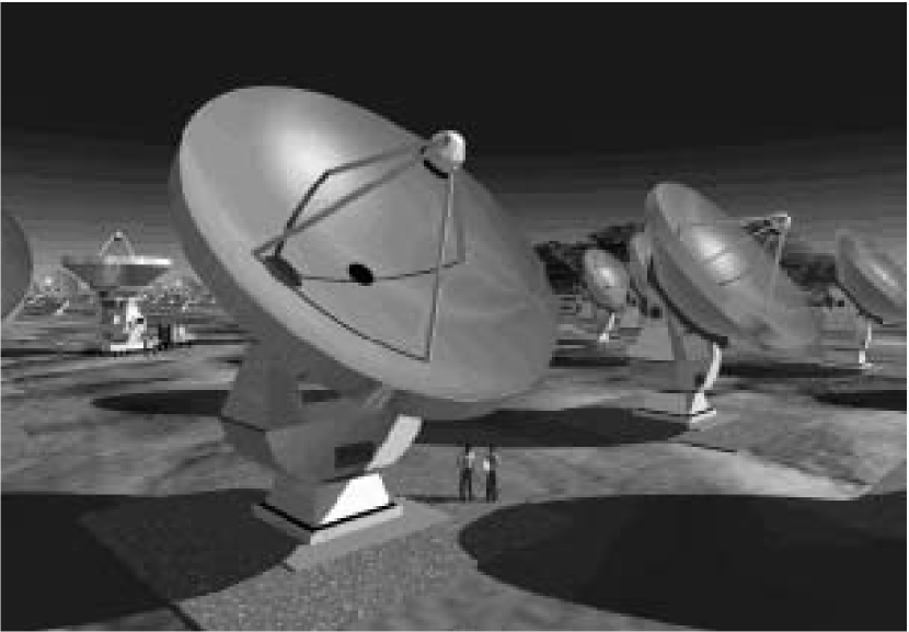
Figure 6: An artists sketch of ALMA. To date, this is the most ambitious construction project in ground based astronomy. ALMA is now being built in north Chile on a 5 km high site. It will consist of fifty-four 12-m and twelve 7-m antennas, operating in 10 bands between wavelength 1 cm and 0.3 mm. In Early Science, four receiver bands at 3, 1.3, 0.8 and 0.6 mm will be available. The high ALMA sensitivity is due to the extremely low noise receivers, the highly accurate antennas, and the high altitude site. At the largest antenna spacing, and shortest wavelength, the angular resolution will be $\sim$5 milliarcseconds (courtesy ESO/NRAO/NAOJ).

6.3.1 Interferometric Observations

Usually measurements are carried out in 1 of 4 ways.

1. Measurements of a single target source. This is similar to the case of single telescope position switching. Two significant differences with single dish measurements are that the interferometer measurement may have to extend over a wide range of hour angles to provide a better coverage of the $(u,v)$ or Fourier plane, and that instrumental phase must be determined also. After the measurement of a calibration source or reference source, which has a known position and size, the effect of instrumental phases in the instrument and atmosphere is removed and a calibration of the amplitudes of the source is made. Target sources and calibrators are usually observed alternately; the calibrator should be close to the target source. The time variations caused by instrumental and weather effects must be slower than the time between measurements of source and calibrator. If, as is the case for mm/sub-mm wavelength measurements, weather is an important influence, target and calibration source must be measured often. For ALMA (see Fig. 6), observing will follow a two part scheme. For fast switching there will be integrations of perhaps 10 seconds on a nearby calibrator, then a few minutes on-source. This method will reduce the amount of phase fluctuations, at the cost of on-source observing time. For more rapid changes in the earth’s atmosphere, phases will be corrected using measurements of atmospheric water vapor from measurements of the 183 GHz line.

2. Snapshot Mode. A series of short observations (at different hour angles) of one source after another, and then the measurements are repeated. For sensitivity reasons, snapshots are usually made in the radio continuum or more intense spectral lines. As in observing method (1), measurements of source and calibrator are interspersed to remove the effects of instrumental phase drifts and to calibrate the amplitudes of the sources in question. The images will affected by the shape of the synthesized beam since there is sparse coverage in the $(u,v)$ plane. If the size of the source to be imaged is comparable to the primary beam of the individual antennas there should be a correction for the power pattern..

3. Multi-Configuration Imaging Here the goal is the image of a source either with high dynamic range or high sensitivity. Measurements with a number of different interferometer configurations better fill the $uv$ plane. These measurements are taken at different epochs and after calibration, the visibilities are entered into a common data set.

4. Mosaicing An extension of procedure (1) can be used for sources with an extent much larger than the primary antenna beam. These images require measurements at adjacent pointings. This is spoken of as mosaicing. In a mosaic, the antennas are pointed at narby positions. These positions should overlap at the half power power point. The images can be formed separately and then combined to produce an image of the larger region. Another method is to combine the data in the $(u,v)$ plane and then form the image.

6.4 Interferometer Sensitivity

The random noise limit to an interferometer system can be calculated following the method used for a single telescope (Eq. 27). The use of (Eq. 43) provides a conversion from $\Delta T_{\rm RMS}$ to $\Delta S_{\nu}$. collecting area of a single antenna. For an array of $n$ identical antennas, there are $N=n(n-1)/2$ simultaneous pairwise correlations, so the RMS variation in flux density is:

$$\Delta S_{\nu}=\frac{2\,M\,k\,T_{\rm sys}^{*}}{A_{\rm e}\sqrt{2\,N\,t\,\Delta\nu}}\,.$$ (66)

with M$\cong 1$, $A_{\rm e}$ the effective area of each antenna and $T_{\rm sys}^{*}$ given by (Eq. 54). This relation can be recast in the form of brightness temperature fluctuations using the Rayleigh-Jeans relation; then the RMS noise in brightness temperature units is:

$$\Delta T_{\rm B}=\frac{2\,M\,k\,\lambda^{2}\,T_{\rm sys}^{*}}{A_{\rm e}\Omega_{\rm b}\sqrt{2\,N\,t\,\Delta\nu}}\,.$$ (67)

For a Gaussian beam, $\Omega_{\rm mb}=1.133\,\theta^{2}$, so the RMS temperature fluctuations can be related to observed properties of a synthesis image.

Aperture synthesis is based on discrete samples of the visibility function $V(u,v)$, with the goal of the densest possible coverage of the $(u,v)$ or Fourier plane. It has been observed that the RMS noise in a synthesis image obtained by Fourier transforming the $(u,v)$ data is often higher than given by (Eq. 66) or (Eq. 67). Possible causes are: (1) phase fluctuations caused by atmospheric or instrumental instabilities, (2) incomplete sampling of the $(u,v)$ plane, which gives rise to artifacts such as stripe-like features in the images, or (3) grating rings around more intense sources; these are analogous to high sidelobes in single dish diffraction patterns.

6.5 Corrections of Visibility Functions

6.5.1 Amplitude and Phase Closure

The relation between the measured $\widetilde{V_{ik}}$ visibility and actual visibility $V_{ik}$ is considered linear:

$$\widetilde{V_{ik}}(t)=g_{i}(t)\,g^{*}_{k}(t)\,V_{ik}+\varepsilon_{ik}(t)\;.$$ (68)

Values for the complex antenna gain factors $g_{k}$ and the noise term $\varepsilon_{ik}(t)$ are determined by measuring calibration sources as frequently as possible. Actual values for $g_{k}$ are then computed by linear interpolation. The (complex) gain of the array is obtained by the multiplication of the gains of the individual antennas. If the array consists of $n$ such antennas, $n(n-1)/2$ visibilities can be measured simultaneously, but only $(n-1)$ independent gains $g_{k}$ are needed since one antenna in the array can be taken as a reference. So in an array with many antennas, the number of antenna pairs greatly exceeds the number of antennas. For phase, one must determine $n$ phases. Often these conditions can be introduced into the solution in the form of closure errors. Defining the phases $\varphi,\theta$ and $\psi$ by
$$\begin{array}[]{rcl}\widetilde{V_{ik}}&=&|\widetilde{V_{ik}}|\,{\rm\,e}^{{\rm\,i\,}\varphi_{ik}}\,,\\ G_{ik}&=&|g_{i}|\,|g_{k}|\,{\rm\,e}^{{\rm\,i\,}\theta_{i}}{\rm\,e}^{-{\rm\,i\,}\theta_{k}}\,,\\ V_{ik}&=&|V_{ik}|\,{\rm\,e}^{{\rm\,i\,}\psi_{ik}}\,.\\ \end{array}$$ (69)
From (Eq. 68) the visibility phase $\psi_{ik}$ on the baseline $ik$ will be related to the observed phase $\varphi_{ik}$ by

$$\varphi_{ik}=\psi_{ik}+\theta_{i}-\theta_{k}+\varepsilon_{ik}\,,$$ (70)

where $\varepsilon_{ik}$ is the phase noise. Then the closure phase $\Psi_{ikl}$ around a closed triangle of baseline $ik,kl,li$,

$$\Psi_{ikl}=\varphi_{ik}+\varphi_{kl}+\varphi_{li}=\psi_{ik}+\psi_{kl}+\psi_{li}+\varepsilon_{ik}+\varepsilon_{kl}+\varepsilon_{li}\,,$$ (71)

will be independent of the phase shifts $\theta$ introduced by the individual antennas and the time variations. With this procedure, phase errors can be minimized.

If four or more antennas are used simultaneously, then the closure amplitudes can be formed. These are independent of the antenna gain factors:

$$A_{klmn}=\frac{|V_{kl}||V_{mn}|}{|V_{km}||V_{ln}|}\;.$$ (72)

Both phase and closure amplitudes can be used to improve the quality of the complex visibility function.

At each antenna there is an unknown complex gain factor $g$ with amplitude and phase, the total number of unknowns can be reduced significantly by measuring closure phases and amplitudes. If four antennas are available, 50 % of the phase information and 33 % of the amplitude information can thus be recovered; in a 10 antenna configuration, these ratios are 80 % and 78 % respectively.

6.5.2 Calibrations, Gridding, FFTs, Weighting and Self Calibration

For two antenna interferometers, phase calibration can only be made pair-wise. This is referred to as ^′′baseline based^′′ solutions for the calibration. For a multi-antenna system, ^′′antenna based^′′ solutions are preferred. These are determined by applying phase and amplitude closure for subsets of antennas and then solving for the best fit for each.

Normally the Cooley-Tukey fast Fourier transform algorithm is used to invert (Eq. 65) To apply the simplest version of the FFT, the visibilities must be placed on a regular grid with sizes that are powers of two of the sampling interval. Since the data seldom lie on such regular grids, an interpolation scheme must be used. From the gridded $(u,v)$ data, an image with a resolution corresponding to $\lambda/D$, where $D$ is the array size, is obtained. However, this may still contain artifacts caused by the observing procedure, especially the limited coverage of the ($u,v$) plane. Therefore the dynamic range of such so-called dirty maps is rather small. This can be improved by further analysis.

If the calibrated visibility function $V(u,v)$ is known for the full $(u,v)$ plane both in amplitude and in phase, this can be used to determine the modified (i.e., structure on angular scales finer than $\lambda/D$ are lost) intensity distribution $I^{\prime}(x,y)$ by performing the Fourier transformation (Eq. 65). However, in a realistic situation $V(u,v)$ is only sampled at discrete points and in some regions of the $(u,v)$ plane, $V(u,v)$ is not measured at all. The visibilities can be weighted by a grading function, $g$. For a discrete number of visibilities, a version of (Eq. 65) involving a summation, not an integral, is used to obtain an image with the use of a discrete Fourier transform (DFT):

$$I_{\rm D}(x,y)=\sum_{k}g(u_{k},v_{k})V(u_{k},v_{k}){\rm\,e}^{-2\pi{\rm\,i\,}(u_{k}x+v_{k}y)}\,,$$ (73)

where $g(u,v)$ is a weighting function referred to as the grading or apodisation. $g(u,v)$ can be used to change the effective beam shape and side lobe level. There are two widely used weighting functions: uniform and natural. Uniform weighting uses $g(u_{k},v_{k})=1$, while natural weighting uses $g(u_{k},g_{k})=1/N_{\rm s}(k)$, where $N_{\rm s}(k)$ is the number of data points within a symmetric region of the $(u,v)$ plane. Data which are naturally weighted result in lower angular resolution but give a better signal-to-noise ratio than uniform weighting. But these are only extreme cases. Intermediate weighting schemes are referred to as robust weighting.

Often the reconstructed image $I_{\rm D}$ may not be a particularly good representation of $I^{\prime}$, but these are related by:

$$I_{\rm D}(x,y)=P_{\rm D}(x,y)\otimes I^{\prime}(x,y)\,,$$ (74)

where $I^{\prime}(x,y)$ is the best representation of the source intensity modified by the primary beam shape; it contains only those spatial frequencies $(u_{k},v_{k})$ where the visibility function has been measured. (see (Eq. 65)). The expression for $P_{\rm D}$ is:

$$P_{\rm D}=\sum_{k}g(u_{k},v_{k}){\rm\,e}^{-2\pi{\rm\,i\,}(u_{k}x+v_{k}y)}$$ (75)

this is the response to a point source, or the point spread function PSF for the dirty beam. Thus $P_{\rm D}$ is a transfer function that distorts the image; $P_{\rm D}$ is produced assuming an amplitude of unity and phase zero at each point sampled. This is the response of the interferometer system to a point source. The sum in (Eq. 75) extends over the same positions $(u_{k},v_{k})$ as in (Eq. 73); the sidelobe structure of the beam depends on the distribution of these points.

Amplitude and phase errors scatter power across the image, giving the appearance of enhanced noise. This problem can be alleviated to an impressive extent by the method of self-calibration. This process can be applied if there is a sufficiently intense compact feature in the field contained within the primary beam of the interferometer system. If self-calibration can be applied, the positional information is usually lost. Self-calibration can be restricted to an improvement of phase alone or to both phase and amplitude. Normally, self-calibration is carried in the $(u,v)$ plane. If this method is used on objects with low signal-to-noise ratios, this may lead to a concentration of random noise into one part of the interferometer image (see Cornwell & Fomalont 1989). For measurements of weak spectral lines, self-calibration is carried out using a continuum source in the field. The corrections are then applied to the spectral line data. In the case of intense lines, one of the frequency channels containing the emission is used.

6.5.3 More Elaborate Improvements of Visibility Functions: The CLEANing Procedure

CLEANing is the most commonly used technique to improve single radio interferometer images (Högbom 1974). In addition to its inherent low dynamic range, the dirty map often contains features such as negative intensity artifacts that cannot be real. Another unsatisfactory aspect is that the solution is quite often rather unstable, in that it can change drastically when more visibility data are added.

The CLEAN method approximates the intensity distribution that represents the best image of the source (subject to angular resolution, noise, etc.), $I(x,y)$, by the superposition of a finite number of point sources with positive intensity $A_{i}$ placed at positions $(x_{i},y_{i})$. The goal of CLEAN to determine the $A_{i}(x_{i},y_{i})$, such that

$$I^{\prime\prime}(x,y)=\sum_{i}A_{i}\,P_{\rm D}(x-x_{i},y-y_{i})+I_{\varepsilon}(x,y)\,$$ (76)

where $I^{\prime\prime}$ is the dirty map obtained from the inversion of the visibility function and $P_{\rm D}$ is the dirty beam (Eq. 75). $I_{\varepsilon}(x,y)$ is the residual brightness distribution after decomposition. Approximation (Eq. 76) is considered successful if $I_{\varepsilon}$ is of the order of the noise in the measured intensities. This decomposition must be carried out iteratively.

The CLEAN algorithm is most commonly applied in the image plane. This is an iterative method which functions in the following fashion: (1) find the peak intensity of the dirty image, then subtract a fraction $\gamma$ (the so-called ^′′loop gain^′′) having the shape of the dirty beam from the image, and (2) repeat this $n$ times.

This loop gain has values $0<\gamma<1$ while $n$ is often taken to be 10⁴. The goal is that the intensities of the residuals are comparable to the noise limit. Finally, the resulting model is convolved with a clean beam of Gaussian shape with a FWHP given by the angular resolution expected from $\lambda/D$ where $D$ is the maximum baseline length. Whether this algorithm produces a realistic image depends on the quality of the data and other variables.

6.5.4 More Elaborate Improvements of Visibility Functions: The Maximum Entropy Procedure

The Maximum Entropy Deconvolution Method (MEM) is commonly used to produce a single optimal image from a set of separate but contiguous images (Gull & Daniell 1978). The problem of how to select the ^′′best^′′ image from many possible images which all agree with the measured visibilities is solved by MEM. Using MEM, those values of the interpolated visibilities are selected, so that the resulting image is consistent with all previous relevant data. In addition, the MEM image has maximum smoothness. This is obtained by maximizing the entropy of the image. One definition of entropy is given by

$${\cal H}=-\sum_{i}I_{i}\left[\ln\bigg{(}\frac{I_{i}}{M_{i}}\bigg{)}-1\right]\,,$$ (77)

where $I_{i}$ is the deconvolved intensity and $M_{i}$ is a reference image incorporating all ^′′a priori^′′ knowledge. In the simplest case $M_{i}$ is the empty field $M_{i}={\rm const}>0$, or perhaps a lower angular resolution image.

Additional constraints might require that all measured visibilities should be reproduced exactly, but in the presence of noise such constraints are often incompatible with $I_{i}>0$ everywhere. Therefore the MEM image is usually constrained to fit the data such that

$$\chi^{2}=\sum\frac{|V_{i}-V_{i}^{\prime}|^{2}}{\sigma_{i}^{2}}$$ (78)

has the expected value, where $V_{i}$ is the measured visibility, $V_{i}^{\prime}$ is a visibility corresponding to the MEM image and $\sigma_{i}$ is the error of the measurement.

Acknowledgement: K. Weiler made a thorough review of the text and H. Bond suggested a number of improvements.

References

- (1) Altenhoff, W. J. 1985, The Solar System: (Sub)mm continuum observations in ESO Conf & Workshop Proc No 22 ed by P. Shaver, K. Kjar, (Garching, European Southern Observatory) p. 591
- (2) Baars, J. W. M., Genzel, R., Pauliny-Toth, I. I. K., Witzel, A. 1977 A & A 61, 99
- (3) Baars, J. W. M. 2007, The Parabolic Reflector Antenna in Radio Astronomy and Communication Astrophysics Space Science Library (Heidelberg, Springer-Verlag)
- (4) Bachiller, R., Cernicharo, J., ed. 2008, Science with the Atacama Large Millimeter Array: A New Era for Astrophysics (Heidelberg, Springer-Verlag)
- (5) Baker, A. J. Glenn, J., Harris, A. I., Mangum, J. G. & Yun, M. S. eds. 2007, From Z Machines to ALMA: (Sub)millimeter Spectroscopy of Galaxies Conf. Ser. 75 (San Francisco, Astron Soc of Pacific)
- (6) Begelman, M. & Rees, M. 2009 Gravity’s Fatal Attraction: Black Holes in the Universe (2nd ed., Cambridge, Cambridge Univ. Press)
- (7) Born, M. & Wolf, E. 1965 Principles of Optics (Oxford, Pergamon )
- (8) Bracewell, R. N. 1986, The Fourier Transform and its Application, (2nd ed, New York, McGraw Hill)
- (9) Burke, B. F. & Graham-Smith, F. 2009 An Introduction to Radio Astronomy, (3rd ed, Cambridge, Cambridge Univ. Press)
- (10) Cornwell, T. & Fomalont, E. B. 1989 Self Calibration in Synthesis Imaging in Radio Astronomy, Conf Series vol. 6, ed by R. Perley et al. (San Francisco, Publ. Astron.Soc. Pacific) p. 185
- (11) Crutcher, R. M. 2008 Astrophys. & Sp. Sci. 313, 141
- (12) Dame, T. M., Ungerechts, H., Cohen, R. S., de Geus, E., Grenier, I. A., May, J., Murphy, D. C., Nyman, L.-A., Thaddeus, P. 1987, ApJ 322, 706
- (13) R. H. Dicke 1946, Rev. Sci. Instrum. 17, 268
- (14) D. Downes 1989, Radio Telescopes: Basic Concepts in Diffraction-Limited Imaging with Very Large Telescopes, NATO ASI Series vol 274, D. M. Alloin, J. M. Mariotti eds. (Dordrecht, Kluwer) p. 53
- (15) Dulk, G. 1985 Ann. Rev. A & A 23, 169
- (16) Dutrey, A. ed: 2001 IRAM Millimeter Interferometry Summer School 2 (Grenoble, IRAM)
- (17) Emerson, D., Klein, U., Haslam, C. G. T. 1979 A & A 76, 92
- (18) Gary, D. E. & Keller, C. U. eds. 2004 Solar & Space Weather Astrophysics, Astrophysics & Space Science Lib. 134 (Dordrecht, Kluwer)
- (19) Giovanelli, R. & Haynes, M. P. 1991 Ann. Rev. A & A 29, 499
- (20) Goldsmith, P. F. ed 1988 Instrumentation and Techniques for Radio Astronomy (New York, IEEE Press)
- (21) Goldsmith, P. F. 1994 Quasioptical Systems: Gaussian Beam Quasioptical Propagation and Applications (New York, Wiley-IEEE Press)
- (22) Gull, S. F. & Daniell, G. J. 1978 Nature 272, 68
- (23) Gurvits, L., Frey, S. & Rawlings, S. eds. 2005, Radio Astronomy from Karl Jansky to Microjansky ( Paris, EDP Sciences)
- (24) Harwit, M. 2006 Astrophysical Concepts (4th ed., Heidelberg, Springer)
- (25) Herbst, E. 2001 Chemical Society Reviews 30, 168
- (26) Herbst, E. & Dishoeck, E. van 2009 Ann. Rev. A & A 47, 247
- (27) Hildebrand, R. 1983 Quarterly J. Roy. Astron. Soc. 24, 267
- (28) Högbom, J. 1974 A & A Suppl. 15, 417
- (29) Holland, W. S. et al 1999 MNRAS 303, 659
- (30) Jenkins, F. A. & White, H. E. 2001, Fundamentals of Optics, (4th ed, New York, McGraw-Hill)
- (31) Johnstone, D. et al. 2000 ApJ Supp. 131, 505
- (32) Kalberla, P. M. W., Burton, W. B., Hartmann, D., Arnal, E. M., Bajaja, E., Morras, R., Pöppel, W .G. L. 2005 A & A 440, 775
- (33) Kalberla, P. M. W. et al. 2010 A & A 521, 17
- (34) Kawamura, J. et al. 2002 A & A 394, 271
- (35) Kellermann, K. I. & Moran, J. M. 2001 Ann. Rev. A & A 39, 457
- (36) Kirshner, R. P. 2004 The Extravagant Universe (Princeton, Princeton Univ. Press)
- (37) Lequeux, J. 2004, The Interstellar Medium (Heidelberg, Springer-Verlag)
- (38) Longair, M. 2006 The Cosmic Century (Cambridge, Cambridge Univ. Press)
- (39) Lorimer, D. & Kramer, M. 2004 Handbook of Pulsar Astronomy (Cambridge, Cambridge Univ. Press)
- (40) Love, A. W. ed. 1976, Electromagnetic Horn Antennas (New York, IEEE Press)
- (41) Lyne, A. G. & Graham-Smith, F. 2006 Pulsar Astronomy (3rd ed, Cambridge, Cambridge Univ. Press)
- (42) Morris, D. 1978 A & A 67, 221
- (43) Motte, F., Bontemps, S., Schneider, N., Schilke, P., Menten, K. M. & Broguierè, D. 2006 A. & A. 476, 1243
- (44) Ott, M. et al. 1994 A & A 284, 331
- (45) Pardo, J. R., Cernicharo, J., Serabyn, E. & Wiedner, M. C. 2009 in ASP Conf. Ser. 417, Submillimeter Astrophysics & Technology, eds. D. C. Lis et al. (San Francisco, Publ. Astron.Soc. Pacific), p 125
- (46) Penzias, A. A. & Wilson, R. W. 1965 ApJ 142, 419
- (47) Penzias, A. A. & Burrus, C. A. 1973 Ann. Rev. A & A 11, 51
- (48) Phillips, T. G. & Woody, D. P. 1982 Ann. Rev. A& A 20, 285
- (49) Reipurth, B., Jewett, D., Keil, K. eds. 2007 Protostars and Planets V (Tucson, Univ of Arizona Press)
- (50) Reich, W., Kalberla, P., Reif, K. & Neidhöfer, J. 1978 A & A 76, 92
- (51) Reid, M. J. 1993 Ann. Rev. A & A 31, 345
- (52) Rieke, G. H. 2002 Detection of Light: From Ultraviolet to the Submillimeter, (2nd ed, Cambridge, Cambridge Univ Press)
- (53) Rohlfs, K., & Wilson, T. L. 2004 Tools of Radio Astronomy, (4th ed, Heidelberg, Springer-Verlag)
- (54) Rybicki, G. B. & Lightman, A. P. 1979, Radiative Processes in Astrophysics ( New York, Wiley)
- (55) Sandell, G. 1994, MNRAS 271, 75
- (56) Silk, J. 2008 The Infinite Cosmos (Oxford, Oxford Univ. Press)
- (57) Solomon, P. M. & Vanden Bout, P. A. 2005 Ann. Rev. A& A 43, 677
- (58) Sparke, L. & Gallagher, J. S. III 2007, Galaxies in the Universe: An Introduction (2nd ed., Cambridge, Cambridge Univ. Press)
- (59) Stahler, S. W. & Palla, F. 2005, The Formation of Stars (New York, Wiley-VCH)
- (60) Sullivan, W. T. III 2005, The Early Years of Radio Astronomy: Reflections 50 Years after Jansky’s Discovery (Cambridge, Cambridge Univ. Press)
- (61) Sullivan, W. T. III 2009 Cosmic Noise, A History of Early Radio Astronomy (Cambridge, Cambridge Univ. Press)
- (62) Taylor, G. B., Carilli, C. L. & Perley, R. A. eds., 1999, ASP Conf. Ser. 180, Synthesis Imaging in Radio Astronomy II (San Francisco, Publ. Astron.Soc. Pacific)
- (63) Thum, C., Wiesemeyer, H., Paubert, G., Navarro, S. & Morris, D. 2008 Publ. Astron.Soc. Pacific 120, 777
- (64) Tielens, A. G. G. M. 2005, The Physics and Chemistry of the Interstellar Medium (Cambridge, Cambridge Univ. Press)
- (65) Thompson, A. R., Moran, J. M. & Swenson, G. W. 2001, Interferometry and Synthesis in Radio Astronomy (2nd ed, New York, Wiley-VCH )
- (66) Townes, C. H. Schawlow, A. H. 1975, Microwave Spectroscopy (New York, Dover)
- (67) Venkata, U. R. 2010 PhD thesis: Parameterized Deconvolution for Wide-Band Radio Synthesis Imaging (Socorro, New Mexico Inst. of Mining & Technology)
- (68) Wilson, T. L., Rohlfs, K. & Hüttemeister, S. 2008, Tools of Radio Astronomy, (5th ed, Heidelberg, Springer-Verlag)