Error estimates for shock capturing finite element approximations of the one dimensional Burgers’ equation

Abstract

We propose an error analysis in weak norms of a shock capturing finite element method for the Burgers’ equation. The estimates can be related to estimates of certain filtered quantities and are robust in the inviscid limit. Using a total variation apriori bound on the discrete solution and an interpolation inequality error estimates in $L^{p}$-norms can are obtained using interpolation.

1 Introduction

There exists a vast litterature on the design and convergence of numerical methods for nonlinear scalar conservation laws dating back to the seminal work of Krushkov [25]. Error estimates are obtained using entropy stability and the so-called variable doubling technique. Asymptotic results have also been obtained using entropy stability and compensated compactness.

For work on convergence and error estimates using finite difference methods we refer to [25, 27, 14, 16, 29, 13, 17, 28], using finite volume methods to [11, 12, 7] and finally for work on finite element methods see [23, 24, 8, 30].

For an introduction to these techniques we refer to the review article by Cockburn [10] or the one by Tadmor [32].

In this work we adopt a strategy that is reminiscent of the negative norm estimates introduced by Tadmor and Nessyahu in [29]. The key argument of their analysis is to use a duality argument to get continuous dependence on initial data for the adjoint perturbation equation of the Burgers’ equation in the $Lip^{\prime}$-norm, i.e. the norm associated to the dual of the space of Lipschitz-continuous functions. Provided the numerical scheme has certain stability properties, in particular that the discrete solution satisfies the discrete maximum principle and the Oleinik E-condition (see [31], this continuous dependence estimate leads to estimates in a weak norm. Estimates in general $L^{p}$-norms may then be recovered using interpolation.

Here we combine these ideas with the theory of dual weighted a posteriori error estimates for finite element methods [24, 21] for the viscous Burgers’ equation in one space dimension. For a shock-capturing finite element method propose to estimate the error of certain filtered quantities associated to weighted weak norms [2]. Indeed we apply the following differential filter to the error,

$$-\delta^{2}\partial_{xx}\tilde{u}+\tilde{u}=u(\cdot,T)\quad\mbox{on }I$$ (1)

with periodic boundary conditions on $\tilde{u}$ and $\partial_{x}\tilde{u}$. The coefficient $\delta$ is proportional to the filter width. Equation (1) naturally leads to the error norm

$$|\|\tilde{u}-\tilde{u}_{h}\||_{\delta}:=\left(\|\delta\partial_{x}(\tilde{u}-\tilde{u}_{h})\|^{2}+\|\tilde{u}-\tilde{u}_{h}\|^{2}\right)^{\frac{1}{2}}$$

where $\|\cdot\|$ denotes the $L^{2}$-norm. We prove an a posteriori error estimate for this norm, proving boundedness of the stability factors. The errors in the filtered quantities can be associated to the estimation of certain weighted averages using a weight function in $H^{1}$.

For the discretization we will consider two different stabilized finite element methods. In both cases the standard Galerkin method (with diagonal mass for the time derivative) is supplemented with a term of artificial viscosity type. First the classical linear artifical viscosity resulting in a first order scheme, related to classical upwind schemes for finite elements and vertex cell finite volume methods and then a weakly consistent nonlinear viscosity in the spirit of that proposed in [4]. The latter is a shockcapturing technique related to those proposed in [23] or the entropy viscosity of [19]. A key observation of this work is that the dual stability required for the error estimates leads to design criteria that have to be satisfied by the shock-capturing term.

Our main result then follows by using the discrete stability of the numerical scheme to upper bound the residuals of the a posteriori estimate resulting in the following error estimate

$$\|\delta\partial_{x}(\tilde{u}-\tilde{u}_{h})(T)\|_{L^{2}(I)}+\|(\tilde{u}-\tilde{u}_{h})(T)\|_{L^{2}(I)}\leq\tilde{C}(u_{0},T)\exp({D_{0}T})\left(\frac{h}{\delta^{2}}\right)^{\frac{1}{2}}$$ (2)

where $\tilde{u}$ and $\tilde{u}_{h}$ are the filtered exact and computational solution respectively. The constant in (2) depend only on the intial data, the mesh geometry and the final time. We will use the notation $U_{0}:=\sup_{x\in I}|\pi_{h}u_{0}(x)|$ and $D_{0}:=\sup_{x\in I}\tfrac{1}{2}\partial_{x}(u_{0}+\pi_{h}u_{0}(x))$, where $\pi_{h}$ denotes the $L^{2}$-projection onto the finite element space. We will choose $u_{0}$ as a smooth function and by the stability of the $L^{2}$-projection on regular meshes we have $U_{0}\lesssim\sup_{x\in I}|u_{0}(x)|$ and $D_{0}\lesssim\sup_{x\in I}|\partial_{x}u_{0}(x)|$, so that estimates depending on $U_{0}$ and $D_{0}$ are indeed mesh independent. Here and in the following we use the notation $a\lesssim b$ defined by $a\leq Cb$ with $C$ a constant independent of $h$, the physical parameters (except if they can be assumed to make an $O(1)$ contribution) and of the exact solution. We will also use $a\sim b$ for $a\lesssim b$ and $b\lesssim a$. For simplicity we assume $u_{0}\in C^{\infty}(I)$, with all the derivatives matcing across the periodic boundaries, this does not exclude the formation of sharp layers with gradients of order $\nu^{-1}$ at later times.

The derivation of the estimate (2) uses:

• stability estimates for the finite element method,

• maximum principles for the finite element solution and its first derivative,

• a priori stability estimates on a linearized dual problem with regularized data,

• Galerkin orthogonality and approximability.

Using a Galiardo-Nirenberg interpolation estimate and the previous stability and error estimates we also obtain the following error estimate in the $L^{p}$-norm

$$\|(u-u_{h})(\cdot,t)\|_{L^{p}(I)}\leq Ch^{\frac{1}{3p}},\,\forall t>0.$$ (3)

The constant depends on the all the constants of the previous estimates, but is independent of the viscosity.

All these results are obtained for the semi-discretization in space only. The extension to the fully discrete case is straightforward in the case of linear artificial viscosity using previous results on finite difference methods, but not so immediate when nonlinear viscosity is used. Indeed in the latter case implicit schemes require regularization of the nonlinearity and the effect of which must be assessed and for explicit schemes, even $L^{2}$-stability for nonlinear viscosity methods is relatively recent [1]. We therefore leave this aspect for future work.

2 The Burgers’ equation with dissipation

Consider the simple model case of the Burgers’ equation with periodic boundary conditions, on the space-time domain $Q:=I\times(0,T)$, with $I:=(0,1)$

$$\begin{array}[]{rcl}\partial_{t}u+\frac{1}{2}\partial_{x}u^{2}-\nu\partial_{xx}u&=&0\mbox{ in }Q\\[8.53581pt] u(0,t)&=&u(1,t)\mbox{ for }t\in(0,T)\\[8.53581pt] \partial_{x}u(0,t)&=&\partial_{x}u(1,t)\mbox{ for }t\in(0,T)\\[8.53581pt] u(x,0)&=&u_{0}(x)\mbox{ for }x\in I.\end{array}$$ (4)

The wellposedness of the equation (4) for $\nu\geq 0$ is well known it is also known that for $\nu>0$ by parabolic regularization the solution is $C^{\infty}(I)$. This high regularity however does not necessarily help us when approximating the solution, since we are interested in computations using a mesh-size that is much larger than the viscosity and still want the bounds to be independent of high order Sobolev norms of the exact solutions and of $\nu$. Let us first show how standard $L^{2}$-energy arguments fail when sharp gradients develop in the solution.

2.1 $L^{2}$-stability of Burgers’ equation

Consider a general perturbation $\eta(x)$ of the initial data of (4).

$$\begin{array}[]{rcl}\partial_{t}\hat{u}+\frac{1}{2}\partial_{x}\hat{u}^{2}-\nu\partial_{xx}\hat{u}&=&0\mbox{ in }Q\\[8.53581pt] \hat{u}(0,t)&=&\hat{u}(1,t)\mbox{ for }t\in(0,T)\\[8.53581pt] \partial_{x}\hat{u}(0,t)&=&\partial_{x}\hat{u}(1,t)\mbox{ for }t\in(0,T)\\[8.53581pt] \hat{u}(x,0)&=&u_{0}(x)+\eta(x)\mbox{ for }x\in I.\end{array}$$ (5)

Taking the difference of (5) and (4) leads to the perturbation equation for $\hat{e}:=\hat{u}-u$ with $a(u,\hat{u}):=\tfrac{1}{2}(u+\hat{u})$,

$$\begin{array}[]{rcl}\partial_{t}\hat{e}+\partial_{x}(a(u,\hat{u})\hat{e})-\nu\partial_{xx}\hat{e}&=&0\mbox{ in }Q,\\[8.53581pt] \hat{e}(0,t)&=&\hat{e}(1,t)\mbox{ for }t\in(0,T)\\[8.53581pt] \partial_{x}\hat{e}(0,t)&=&\partial_{x}\hat{e}(1,t)\mbox{ for }t\in(0,T)\\[8.53581pt] \hat{e}(x,0)&=&\eta(x)\mbox{ for }x\in I.\end{array}$$ (6)

Multiplying equation (6) by $\hat{e}$ and integrating over $Q$ leads to the energy equality

$$\frac{1}{2}\|\hat{e}(T)\|_{L^{2}(I)}^{2}+\|\nu^{\frac{1}{2}}\partial_{x}\hat{e}\|^{2}_{L^{2}(Q)}=\frac{1}{2}\|\eta\|_{L^{2}(I)}^{2}-\frac{1}{2}\int_{Q}(\partial_{x}a(u,\hat{u}))\hat{e}^{2}.$$

We know that due to shock formation $\|\partial_{x}a(u,\hat{u})\|_{L^{\infty}(I)}\sim\nu^{-1}$ [31]. Any attempt to obtain control of $\|\hat{e}(T)\|_{L^{2}(I)}^{2}$ in terms of the initial data will rely on Gronwall’s lemma, leading to

$$\|\hat{e}(T)\|_{L^{2}(I)}^{2}\leq C_{a}\|\eta\|_{L^{2}(I)}^{2}$$

with the exponential factor

$$C_{a}:=\exp({\|\partial_{x}a(u,\hat{u})\|_{L^{\infty}(Q)}T})\sim\exp(T/\nu).$$

This factor obviously makes the estimate meaningless for large gradients/small viscosities. It tells us that the energy method only gives us useful information on the stability up to the formation of shocks. Using this type of argument in the analysis of the finite element method leads to error estimates of the type derived in [6], useful only for solutions with moderate gradients.

2.2 Maximum principles for Burgers’ equation

It is well known that the equation (4) satisfies a maximum principle [31] on the form:

$$\sup_{(x,t)\in Q}|u(x,t)|\leq\sup_{x\in I}|u_{0}(x)|.$$ (7)

This follows using standard techniques recalling the smoothness of the solution $u$ (or in the hyperbolic case, using the method of characteristics). For our purposes we also need some precise information on the derivative. Since the solution of (4) is smooth we may derive the equation in space to obtain the following equation for the space derivative $w:=\partial_{x}u$:

$$\begin{array}[]{rcl}\partial_{t}w+u\partial_{x}w-\nu\partial_{xx}w&=&-w^{2}\mbox{ in }Q\\[8.53581pt] w(0,t)&=&w(1,t)\mbox{ for }t\in(0,T)\\[8.53581pt] \partial_{x}w(0,t)&=&\partial_{x}w(1,t)\mbox{ for }t\in(0,T)\\[8.53581pt] w(x,0)&=&\partial_{x}u_{0}(x)\mbox{ for }x\in I.\end{array}$$ (8)

Assuming that for some time $t>0$ $w$ takes its maximum in some point $x\in I$ and noting that $\partial_{x}w(x,t)=0$ and $\partial_{xx}w(x,t)<0$ it follows that $\partial_{t}w(x,t)<0$ at the maximum and we deduce the bound:

$$\max_{(x,t)\in Q}\partial_{x}u\leq\max_{x\in I}\partial_{x}u_{0}.$$ (9)

It follows by the smoothness of the initial data that the space derivative is bounded above for all times.

3 Artificial viscosity finite element method

Discretize the interval $I$ with $N$ elements and let the local mesh-size be defined by $h:=1/N$. We denote the computational nodes by $x_{i}:=i\,h$, $i=0,\ldots,N$, defining the elements $I_{j}:=[x_{j},x_{j+1}]$, $j=0,\ldots,N-1$, and the standard nodal basis functions $\{v_{i}\}_{i=0}^{N}$, such that $v_{i}(x_{j})=\delta_{ij}$, with $\delta_{ij}$ the Kronecker delta. To impose periodic boundary conditions we identify the node $x_{0}$ with $x_{N}$ and define the corresponding basis function $v_{0N}:(x_{0},x_{1})\cup(x_{N-1},x_{N})\mapsto\mathbb{R}$ by $v_{0}$ on $(x_{0},x_{1})$ and by $v_{N}$ on $(x_{N-1},x_{N})$. This basis function then replaces $v_{0}$ and $v_{N}$, leading to a total of $N$ degrees of freedom. For simplicity we use the notation $v_{0}$ for the basis function $v_{0N}$. The finite element space is given by

$$V_{h}:=\left\{\sum_{i=0}^{N-1}u_{i}v_{i},\mbox{ where }\{u_{i}\}_{i=0}^{N-1}\in\mathbb{R}^{N}\right\}.$$

We define the standard $L^{2}$ inner product on $X\subset I$ by

$$(v_{h},w_{h})_{X}:=\int_{X}v_{h}w_{h}\,\mbox{d}x.$$

The discrete form corresponding to mass-lumping reads

$$(v_{h},w_{h})_{h}:=\sum_{i=0}^{N-1}v_{h}(x_{i})w_{h}(x_{i})h.$$

The associated norms are defined by $\|v\|_{X}:=(v,v)_{X}^{\frac{1}{2}}$, for all $v\in L^{2}(X)$, if $X$ coincides with $I$ the subscript is dropped, and $\|v_{h}\|_{h}:=(v_{h},v_{h})_{h}^{\frac{1}{2}}$ for all $v_{h}\in V_{h}$. Note that, by norm equivalence on discrete spaces, for all $v_{h}\in V_{h}$ there holds

$$\|v_{h}\|_{h}\lesssim\|v_{h}\|\lesssim\|v_{h}\|_{h}.$$

Using the above notation the artificial viscosity finite element space semi-discretization of (4) reads, given $u_{0}\in C^{\infty}(I)$ find $u_{h}(t)\in V_{h}$ such that $(u_{h}(0),v_{h})_{I}=(u_{0},v_{h})_{I}$ and

$$(\partial_{t}u_{h},v_{h})_{h}+\left(\partial_{x}\frac{u_{h}^{2}}{2},v_{h}\right)_{I}+(\hat{\nu}\partial_{x}u_{h},\partial_{x}v_{h})_{I}=0,\mbox{ for all }v_{h}\in V_{h}\mbox{ and }t>0,$$ (10)

where we propose two different forms of $\hat{\nu}$:

1. linear artificial viscosity:

   $$\hat{\nu}:=\max(U_{0}h/2,\nu);$$ (11)

2. nonlinear artificial viscosity:
   Let $0\leq\epsilon$ and

   $$\nu_{0}(u_{h})|_{I_{i}}:=\frac{1}{2}\|u_{h}\|_{L^{\infty}(I_{i})}\max_{x\in\{x_{i},x_{i+1}\}}\frac{|[\![\partial_{x}u_{h}]\!]|_{x}|}{2\{|\partial_{x}u_{h}|\}|_{x}+\epsilon},$$ (12)

   where $[\![\partial_{x}u_{h}]\!]|_{x_{i}}$ denotes the jump of $\partial_{x}u_{h}$ over the node $x_{i}$ and $\{|\partial_{x}u_{h}|\}|_{x_{i}}$ denotes the average of $|\partial_{x}u_{h}|$ over $x_{i}$. If $\epsilon=0$ and $\{|\partial_{x}u_{h}|\}|_{x_{i}}=0$ we replace the quotient $|[\partial_{x}u_{h}]|_{x_{i}}|/\{|\partial_{x}u_{h}|\}|_{x_{i}}$ by zero.

   Further let

   $$\xi(u_{h})|_{I_{i}}:=\left\{\begin{array}[]{ll}1\quad\mbox{if $\partial_{x}u_{h}|_{I_{i}}>0$, $\partial_{x}u_{h}|_{I_{i}}>\partial_{x}u_{h}|_{I_{i+1}}>0$}\\ \quad\mbox{ and $\partial_{x}u_{h}|_{I_{i}}\geq\partial_{x}u_{h}|_{I_{i-1}}>0$}\\ 0\quad\mbox{otherwise}\end{array}\right.$$

   $$\nu_{1}(u_{h})|_{I_{i}}:=\xi(u_{h})|_{I_{i}}\frac{1}{2}(\nu_{0}|_{I_{i-1}}\frac{\partial_{x}u_{h}|_{I_{i-1}}}{\partial_{x}u_{h}|_{I_{i}}}+\nu_{0}|_{I_{i+1}}\frac{\partial_{x}u_{h}|_{I_{i+1}}}{\partial_{x}u_{h}|_{I_{i}}}\Bigr{)}.$$ (13)

   Finally define:

   $$\hat{\nu}(u_{h})|_{I_{i}}:=\max(\nu,h(\nu_{0}|_{I_{i}}+\nu_{1}|_{I_{i}})).$$ (14)

The rationale for the nonlinear viscosity is to add first order viscosity at local extrema of the solution $u_{h}$ so that (7) holds also for the discrete solution and enough viscosity at positive extrema of $\partial_{x}u_{h}$, making (9) carry over to the discrete setting. The most important term is $\nu_{0}$, ensuring the discrete maximum principle. The other part $\nu_{1}$ is merely a correction that ensures that the viscosity at local maxima of $\partial_{x}u_{h}$ dominates that of the surrounding elements. Indeed the role of the function $\xi(u_{h})$ is to act as an indicator function for the elements where the local maxima of $\partial_{x}u_{h}$ are taken and modify the viscosity there. By construction, if $\xi(u_{h})=1$ in one element it must be zero in the neighbouring elements. Note that formally $\hat{\nu}(u_{h})\approx O(\max(U_{0}h^{3/2}),\nu)$ in the smooth part of the solution, so that in principle we can expect higher order convergence away from local extrema. Note that the perturbation $\nu_{1}$ close to extrema of the gradient of the solution has no impact on the formal order. The high order convergence properties and the effect of the regularization parameter $\epsilon$ will be explored in the numerical section.

Remark 1.

Note that in the linear case the viscosity $\hat{\nu}$ may be written as

$$\hat{\nu}:=\nu\max(1,Re_{h}),\quad\mbox{ with }Re_{h}:=\frac{U_{0}h}{2\nu}$$

reflecting that in the high Reynolds number regime the viscosity is increased artificially to be order $h$.

3.1 Existence of solution to the semidiscretized system

For the linear method existence and uniqueness of solutions of (10) follows using standard methods. First we observe that the nonlinear function of the dynamical system is locally Lipschitz and then anticipating the global upper bound (15) we conclude that a global solution exists and is unique.

The nonlinear method obtained when (10) is used with the viscosity (14) results in a dynamical system with discontinuous righthand side (even for $\epsilon>0$ the contribution from $\nu_{1}$ introduces discontinuities). Existence of solutions to (10) with the nonlinear viscosity (14) is obtained using Filippov theory [18]. Anticipating the results of the next section, we may conclude that a solution exists, since by the discrete maximum principle (15), for fixed $h$, there holds

$$\Bigl{|}\left(\partial_{x}\frac{u_{h}^{2}}{2},v_{i}\right)_{I}+(\hat{\nu}\partial_{x}u_{h},\partial_{x}v_{i})_{I}\Bigr{|}\leq M\|v_{i}\|_{L^{2}(I)}$$

and hence $|\partial_{t}u_{h}(x,t)|<M$ for all $(x,t)\in Q$. The question of uniqueness is more involved, but we conjecture that the solution is forward unique since by construction it satisfies the Oleinik E-condition. Indeed the decrease of the maximum derivative by construction, rules out the so called repulsive sliding mode that is known to cause nonuniqueness of the solution. We will not explore these issues further here but refer the interested reader to [15]. Typically in practice the system (10) will be discretized in time using an explicit time stepping scheme which, by definition, will produce a unique discrete solution. In the following we will prove that any solution to (10) will satisfy certain uniform bounds and converge to the exact solution at a certain rate.

3.2 Maximum principles for the discrete solution

Maximum principles give local estimates of the behavior of the solution and they rarely carry over to the discrete method. There are however stabilized methods that are specially designed to make a discrete maximum principle hold, see for instance [33, 5] for linear convection–diffusion problems and [26, 4] for maximum principle satisfying finite element methods for conservation laws.

In [4] it was shown that the discrete equivalent of (7), together with energy stability of the discrete solution is sufficient to prove the convergence of the approximation sequence to the entropy solution. For our purposes herein however it is not sufficient, but we also need to prove a discrete equivalent of the bound (9) on the gradient. We collect the monotonicity results we need in the following lemma. For clarity of the exposition we first give the proofs in the case $\epsilon=0$ and then discuss how the regularization modifies the bounds.

Lemma 1.

Let $u_{h}$ be the solution of (10) either using the linear viscosity (11) or the nonlinear viscosity (14) and $\epsilon=0$. Then the following bounds hold:

$$\sup_{(x,t)\in Q}|u_{h}(x,t)|\leq U_{0}\lesssim\max_{x\in I}|u_{0}(x)|,$$ (15)

$$\sup_{(x,t)\in Q}\partial_{x}u_{h}(x,t)\leq\max_{x\in I}\partial_{x}u_{h}(x,0)\lesssim\max_{x\in I}|\partial_{x}u_{0}(x)|.$$ (16)

Proof.

The proof of (15) is an immediate consequence of the fact that the space discretization has the DMP-property introduced in [5].

For the case of linear artificial viscosity, first assume that for some time $t^{*}$ there holds $\max_{x\in I}|u_{h}(x,t^{*})|\leq U_{0}$, then show that this implies

$$\max_{t\geq t*}\max_{x\in I}|u_{h}(x,t)|\leq U_{0}$$ (17)

and conclude noting that the assumed inequality holds for $t^{*}=0$, since

$$\max_{x\in I}|u_{h}(x,0)|=:U_{0}.$$

First we compute

$$\int_{I}u_{h}\partial_{x}u_{h}v_{i}~{}\mbox{d}x=\frac{h^{2}}{3}(\partial_{x}u_{h}|_{I_{i-1}})^{2}+\frac{h^{2}}{6}(\partial_{x}u_{h}|_{I_{i}})^{2}\\ +\frac{h}{2}u_{h}(x_{i-1},t^{*})\partial_{x}u_{h}|_{I_{i-1}}+\frac{h}{2}u_{h}(x_{i},t^{*})\partial_{x}u_{h}|_{I_{i}}$$ (18)

Assuming that $u_{h}$ has a local max in $x_{i}$ at $t=t^{*}$ it follows that, for linear viscosity

$$h\partial_{t}u_{h}(x_{i},t^{*})=-(u_{h}\partial_{x}u_{h},v_{i})_{I}-(\hat{\nu}\partial_{x}u_{h},\partial_{x}v_{i})_{I}\\ \leq-\frac{h}{2}\left(U_{0}-\max(|u_{h}(x_{i-1},t^{*})|,|u_{h}(x_{i},t^{*})|)\right)(|\partial_{x}u_{h}|_{I_{i-1}}|+|\partial_{x}u_{h}|_{I_{i}}|)\leq 0.$$

It follows that $\partial_{t}u_{h}(x_{i},t^{*})\leq 0$ and hence the local maximum can not grow. The case of a local minimum is similar.

For nonlinear viscosity on the form (12), since at a local maximum $|[\![[\partial_{x}u_{h}]]\!]|=2\{|\partial_{x}u_{h}\}$, we deduce that

$$\hat{\nu}(u_{h})|_{I_{i}}=\|u_{h}(\cdot,t^{*})\|_{L^{\infty}(I_{i})}h/2=\max(|u(x_{i},t^{*})|,|u(x_{i+1},t^{*})|)h/2$$

and the same conclusion follows. To reduce the notation below we drop the argument $t^{*}$.

We will show (16) by first proving that the maximum gradient must be decreasing, and then applying the stability of the $L^{2}$ projection. Hence it is sufficient to prove that $\partial_{t}\max_{i}\partial_{x}u_{h}|_{I_{i}}\leq 0$ in $Q$ to conclude.

We first give the proof for the linear artificial viscosity. We will prove that the discrete gradient is bounded by the gradient of the discrete initial data.

$$\sup_{(x,t)\in Q}\partial_{x}u_{h}(x,t)\leq\sup_{x\in I}\partial_{x}\pi_{h}u_{0}.$$

Starting from (10), we let $I_{i}$ be any element where $\partial_{x}u_{h}|_{I_{i}}$ has a local maximum, in the sense $\partial_{x}u_{h}|_{I_{i}}\geq\partial_{x}u_{h}|_{I_{i\pm 1}}\geq 0$.

$$\partial_{t}\partial_{x}u_{h}|_{I_{i}}=-\frac{1}{h}\int_{x_{i-1}}^{x_{i+2}}u_{h}\partial_{x}u_{h}(v_{i+1}-v_{i})~{}\mbox{d}x-\\ \frac{1}{h}\int_{x_{i-1}}^{x_{i+2}}\hat{\nu}\partial_{x}u_{h}\partial_{x}(v_{i+1}-v_{i})~{}\mbox{d}x=T_{1}+T_{2}.$$

Decomposing the integral $T_{1}$ on the contributions from $v_{i}$ and $v_{i+1}$ we have using (18) and some minor manipulations

$$T_{1}=-\frac{1}{6}h(\partial_{x}u_{h}|_{I_{i-1}})^{2}-\frac{2}{3}h(\partial_{x}u_{h}|_{I_{i}})^{2}-\frac{1}{6}h(\partial_{x}u_{h}|_{I_{i+1}})^{2}\\ -\frac{1}{2}u_{h}(x_{i})(\partial_{x}u_{h}|_{I_{i}}-\partial_{x}u_{h}|_{I_{i-1}})-\frac{1}{2}u_{h}(x_{i+1})(\partial_{x}u_{h}|_{I_{i+1}}-\partial_{x}u_{h}|_{I_{i}}).$$

Since the derivative takes its max value in $I_{i}$ we have for $T_{2}$

$$T_{2}=-\frac{1}{h}\int_{x_{i-1}}^{x_{i+2}}\hat{\nu}\partial_{x}u_{h}\partial_{x}(v_{i+1}-v_{i})~{}\mbox{d}x\\ =h^{-1}((\hat{\nu}(u_{h})\partial_{x}u_{h})|_{I_{i-1}}-2(\hat{\nu}(u_{h})\partial_{x}u_{h})|_{I_{i}}+(\hat{\nu}(u_{h})\partial_{x}u_{h}|_{I_{i+1}}))\leq 0.$$

Collecting the above expressions and using that $\hat{\nu}\geq\tfrac{1}{2}U_{0}h$, and we obtain

$$T_{1}+T_{2}\leq-\frac{1}{6}h(\partial_{x}u_{h}|_{I_{i+1}})^{2}-\frac{2}{3}h(\partial_{x}u_{h}|_{I_{i}})^{2}-\frac{1}{6}h(\partial_{x}u_{h}|_{I_{i-1}})^{2}\\ -\frac{1}{2}\underbrace{(U_{0}+u_{h}(x_{i}))}_{\geq 0}\underbrace{(\partial_{x}u_{h}|_{I_{i}}-\partial_{x}u_{h}|_{I_{i-1}})}_{\geq 0}\\ -\frac{1}{2}\underbrace{(U_{0}-u_{h}(x_{i+1}))}_{\geq 0}\underbrace{(\partial_{x}u_{h}|_{I_{i}}-\partial_{x}u_{h}|_{I_{i+1}})}_{\geq 0}\leq 0.$$

This proves that $\partial_{t}\max_{i}\partial_{x}u_{h}|_{I_{i}}\leq 0$ and therefore the maximum space derivative is alway decreasing. The global upper bound (16) is immediate by the stability of the $L^{2}$-projection. Note that by the non-monotonicity of the $L^{2}$-projection there is now an absolute value on the derivative of the initial data.

In the case of the nonlinear viscosity given by (14) we first show that the time derivative of the gradient must be negative in cells with $\xi(u_{h})=1$. Then we show that any adjacent element, cannot grow either due to the design of the nonlinear switch. In this case have after integration

$$T_{1}+T_{2}=-\frac{1}{6}h(\partial_{x}u_{h}|_{I_{i+1}})^{2}-\frac{2}{3}h(\partial_{x}u_{h}|_{I_{i}})^{2}-\frac{1}{6}h(\partial_{x}u_{h}|_{I_{i-1}})^{2}\\ +h^{-1}((\hat{\nu}(u_{h})\partial_{x}u_{h})|_{I_{i-1}}-2(\hat{\nu}(u_{h})\partial_{x}u_{h})|_{I_{i}}+(\hat{\nu}(u_{h})\partial_{x}u_{h}|_{I_{i+1}}))\\ -\frac{1}{2}u_{h}(x_{i})(\partial_{x}u_{h}|_{I_{i}}-\partial_{x}u_{h}|_{I_{i-1}})+\frac{1}{2}u_{h}(x_{i+1})(\partial_{x}u_{h}|_{I_{i}}-\partial_{x}u_{h}|_{I_{i+1}}).$$ (19)

First observe that the case where either $x_{i}$ or $x_{i+1}$ is a local extremum can be excluded, since then $\nu_{0}|_{I_{i}}=\tfrac{1}{2}\|u_{h}\|_{L^{\infty}(I)}$ and by observing the sign of the contribution of the derivative from the neighbouring cells in the viscosity terms of line two and three of (19). The other terms are controlled as in the linear theory with minor modifications.

Since the gradient has a local max in $I_{i}$, in the sense that $\xi(u_{h})|_{I_{i}}=1$ there holds

$$\hat{\nu}(u_{h})|_{I_{i}}=\frac{1}{2}(\nu_{0}(u_{h})|_{I_{i-1}}\frac{\partial_{x}u_{h}|_{I_{i-1}}}{\partial_{x}u_{h}|_{I_{i}}}+\nu_{0}(u_{h})|_{I_{i+1}}\frac{\partial_{x}u_{h}|_{I_{i+1}}}{\partial_{x}u_{h}|_{I_{i}}})+\nu_{0}(u_{h})|_{I_{i}}$$

and since by construction $\xi(u_{h})|_{I_{i\pm 1}}=0$, we have in the neighbouring cells,

$$\hat{\nu}(u_{h})|_{I_{i\pm 1}}=\nu_{0}(u_{h})|_{I_{i\pm 1}}.$$

Using the values of $\hat{\nu}$ the contribution from the viscous part of the differential operator may be bounded as

$$(\hat{\nu}(u_{h})\partial_{x}u_{h})|_{I_{i-1}}-2(\hat{\nu}(u_{h})\partial_{x}u_{h})|_{I_{i}}+(\hat{\nu}(u_{h})\partial_{x}u_{h}|_{I_{i+1}})=-2h\nu_{0}(u_{h})|_{I_{i}}\partial_{x}u_{h}|_{I_{i}}.$$ (20)

For the two last terms in the right hand side of (19) we note that, assuming first $u_{h}(x_{i+1})\geq u_{h}(x_{i})\geq 0$,

$$-\frac{1}{2}\underbrace{u_{h}(x_{i})(\partial_{x}u_{h}|_{I_{i}}-\partial_{x}u_{h}|_{I_{i-1}})}_{\geq 0}+\frac{1}{2}u_{h}(x_{i+1})(\partial_{x}u_{h}|_{I_{i}}-\partial_{x}u_{h}|_{I_{i+1}})\\ \leq\nu_{0}(u_{h})|_{I_{i}}(|\partial_{x}u_{h}|_{I_{i}}|+|\partial_{x}u_{h}|_{I_{i+1}}|)$$ (21)

Collecting (20) and (21), (19) can be upper bounded in the following fashion, recalling that $\partial_{x}u_{h}|_{I_{i}}>\partial_{x}u_{h}|_{I_{i+1}}>0$:

$$T_{1}+T_{2}\leq-\frac{1}{6}h(\partial_{x}u_{h}|_{I_{i+1}})^{2}-\frac{2}{3}h(\partial_{x}u_{h}|_{I_{i}})^{2}-\frac{1}{6}h(\partial_{x}u_{h}|_{I_{i-1}})^{2}\\ -2\nu_{0}(u_{h})|_{I_{i}}\partial_{x}u_{h}|_{I_{i}}+\nu_{0}(u_{h})|_{I_{i}}(|\partial_{x}u_{h}|_{I_{i}}|+|\partial_{x}u_{h}|_{I_{i+1}}|)\leq 0.$$ (22)

The case $0\geq u_{h}(x_{i+1})\geq u_{h}(x_{i})$ is similar observing that in that case the last term in the right hand side of (19) is negative. In case $u_{h}(x_{i})<0<u_{h}(x_{i+1})$ we observe that only the treatment of the first contribution of the last line of (19) must be modified. We note that

$$-\frac{1}{2}u_{h}(x_{i})(\partial_{x}u_{h}|_{I_{i}}-\partial_{x}u_{h}|_{I_{i-1}})\\ \leq\frac{1}{2}h(\partial_{x}u_{h}|_{I_{i}})^{2}$$

and that this term is cancelled by the second term of the right hand side in the first line of (19).

Finally we must check that the gradient can not increase in any portion of the domain where the gradient is constant at the maximum value over several elements from $I_{m}$ to $I_{n}$, $m<n$, at some time $t^{*}$. First note that for all elements $I_{m+2},...,I_{n-2}$ the derivative is decreasing, since only the first three terms of the right hand side of (19) are non-zero. By construction $\xi(u_{h})|_{I_{n}}=1$ and hence the derivative is decreasing in $I_{n}$. As a consequence the derivative in $I_{n-1}$ is either decreasing at the time $t^{*}$ or will have $\xi|_{I_{n-1}}=1$ at $t^{*}+\varepsilon$ for all $\varepsilon>0$ and hence be non-increasing. Similarly for $I_{m}$ and $I_{m+1}$, the derivatives can not grow at the same rate in both cells since then $\xi|_{I_{m+1}}=1$ at $t^{*}+\varepsilon$ for all $\varepsilon>0$, since its right hand side neighbour has decreasing space derivative. If, on the other hand the time derivative of the derivative is the largest in $I_{m}$ at time $t=t^{*}$ then $\xi|_{I_{m}}=1$ at $t^{*}+\varepsilon$ for all $\varepsilon>0$, and hence the derivative can not grow. This case of several adjacent cells over which the gradient is constant is what can give rise to the so called attractive sliding mode in the Filippov theory. ∎

Remark 2.

First observe that if $\nu_{1}=0$ it is not difficult to find $u_{h}$ for which $\partial_{t}\max_{i}\partial_{x}u_{h}|_{I_{i}}>0$, so the above technique of proof requires the contribution from $\nu_{1}$, whether or not it is really necessary in practice remains unclear.

It was shown in [4] that a consequence of the bound (1) is that the total variation of $u_{h}$ diminuishes. We recall the result without proof.

Corollary 2.

Let $u_{h}$ be the solution of (10), then there holds, for all $t\geq 0$

$$TV(u_{h}(\cdot,t)):=\int_{I}|\partial_{x}u_{h}(\cdot,t)|~{}\mbox{d}x\leq TV(u_{h}(\cdot,0)).$$

3.2.1 The effect of non-zero regularization parameter $\epsilon$

In practice it may be practical to use a value on $\epsilon$ that is related to the mesh size, in particular if implicit solvers are used it is known that the regularized shock-capturing term has smoother convergence properties. This will result in a modification of the upper bounds (15) and (16), but as we show below, the maximum principles can only be violated by an $\mathcal{O}(\epsilon)$.

Proposition 3.

Let $0<\epsilon T<1$ in (12), let $u_{h}$ be the solution of (10), then there holds

$$\|u_{h}(\cdot,T)\|_{L^{\infty}(I)}\leq(1+\epsilon T)U_{0}$$ (23)

and

$$\max_{(x,t)\in Q}\partial_{x}u_{h}(x,t)\leq\max_{x\in I}\partial_{x}u_{h}(x,0)+U_{0}(1+\epsilon T)\epsilon T.$$ (24)

Proof.

Assume for simplicity that $u_{h}\geq 0$ and that $u_{h}$ takes a global (positive) maximum in $x_{i}$ that will grow with the maximum rate throughout the computation. Introduce the notation

$$g_{1}:=|\partial_{x}u_{h}|_{I_{i-1}}|,\quad g_{2}:=|\partial_{x}u_{h}|_{I_{i}}|.$$

Recall that at a local maximum of $u_{h}$, $\xi(u_{h})=0$ and therefore $\hat{\nu}(u_{h})=\max(\nu,\nu_{0}(u_{h}))$. Assume that the maximum is taken for $\nu_{0}(u_{h})$. Then by (18)

$$\partial_{t}u_{h}(x_{i})\leq\frac{1}{2}u_{h}(x_{i})(g_{1}+g_{2})-h^{-1}\hat{\nu}_{h}(u_{h})|_{I_{i-1}}g_{1}-h^{-1}\hat{\nu}_{h}(u_{h})|_{I_{i}}g_{2})\\ \leq\frac{1}{2}u_{h}(x_{i})(g_{1}+g_{2}-\frac{(g_{1}+g_{2})^{2}}{g_{1}+g_{2}+\epsilon})\leq\frac{1}{2}u_{h}(x_{i})\epsilon.$$

By Gronwall’s lemma it follows that

$$u_{h}(x_{i},T)\leq U_{0}e^{\frac{1}{2}\epsilon T}.$$

Since $e^{x}<1+x/(1-x)$ we conclude, using the assumption that $\epsilon T<1$,

$$u_{h}(x_{i},T)\leq U_{0}(1+\epsilon T).$$

To obtain the inequality (24) we reason in a similar fashion starting from the equation (19) and using (23). The regularization only comes into effect at the step (21) and we observe that in this case

$$-\frac{1}{2}u_{h}(x_{i})(\partial_{x}u_{h}|_{I_{i}}-\partial_{x}u_{h}|_{I_{i-1}})+\frac{1}{2}u_{h}(x_{i+1})(\partial_{x}u_{h}|_{I_{i}}-\partial_{x}u_{h}|_{I_{i+1}})\\ \leq\nu_{0}(u_{h})|_{I_{i}}(|\partial_{x}u_{h}|_{I_{i}}|+|\partial_{x}u_{h}|_{I_{i+1}}|+\epsilon).$$ (25)

This then leads to the bound

$$\partial_{t}\partial_{x}u_{h}|_{I_{i}}\leq-\frac{1}{6}h(\partial_{x}u_{h}|_{I_{i+1}})^{2}-\frac{2}{3}h(\partial_{x}u_{h}|_{I_{i}})^{2}-\frac{1}{6}h(\partial_{x}u_{h}|_{I_{i-1}})^{2}+\frac{1}{2}u_{h}(x_{i+1})\epsilon.$$

Integrating in time shows that

$$\max_{(x,t)\in Q}\partial_{x}u_{h}\leq\max_{x\in I}\partial_{x}u_{h}(x,0)+U_{0}(1+\epsilon T)\epsilon T.$$

∎

A regularization of $\xi_{h}$ can also be performed and analysed with similar outcome for the estimate (16). These perturbations of the discrete maximum principle then modifies the result (2). Assuming that the maximum violation takes place in every node in the mesh it is straightforward to show that the total variation remains upper bounded uniformly in $h$ and with linear growth in $T$, provided $\epsilon\leq O(h)$.

3.3 Energy stability

Our estimates rely on stability of the numerical scheme and regularity of the dual perturbation equation. We need to control certain Sobolev norms of the discrete solution in energy type estimates similar to that of the continuous problem. The proof of the below estimates can be simplified in the linear case and the inverse estimate on the $L^{\infty}$-norm that is only valid in one dimension can then be avoided. Here we only give the proof valid both in the linear and in the nonlinear case.

Lemma 4.

The solution $u_{h}$ of the formulation (10) with either the linear artificial viscosity given by (11) or the nonlinear one of (14) with $\epsilon=0$, satisfies the upper bounds

$$\|u_{h}(T)\|+\|\hat{\nu}^{\frac{1}{2}}\partial_{x}u_{h}\|_{Q}\lesssim\|u_{0}\|$$ (26)

$$\|\partial_{t}u_{h}\|_{Q}\lesssim(U_{0}T^{\frac{1}{2}}h^{-\frac{1}{2}}+\nu^{\frac{1}{2}})\|\partial_{x}u_{0}\|.$$ (27)

Proof.

The estimate (26) is immediate by taking $v_{h}=u_{h}$ and noticing, by integration by parts and the periodic boundary conditions, that the nonlinear transport term vanishes. By norm equivalence and the stability of the $L^{2}$-projection

$$\|u_{h}(T)\|\lesssim\|u_{h}(T)\|_{h}\mbox{ and }\|u_{h}(0)\|_{h}\lesssim\|u_{0}\|.$$

The second estimate follows by taking $v_{h}=\partial_{t}u_{h}$ to obtain

$$\int_{0}^{T}\|\partial_{t}u_{h}\|_{h}^{2}~{}\mbox{d}t=-\int_{0}^{T}(u_{h}\partial_{x}u_{h},\partial_{t}u_{h})_{I}~{}\mbox{d}t-\int_{0}^{T}(\hat{\nu}\partial_{x}u_{h},\partial_{x}\partial_{t}u_{h})_{I}~{}\mbox{d}t.$$ (28)

First note that by Corollary 2 and (15) we have, since $TV(u_{h})\leq\mbox{meas}(I)^{\frac{1}{2}}\|\partial_{x}u_{h}\|$,

$$\int_{0}^{T}(u_{h}\partial_{x}u_{h},\partial_{t}u_{h})_{I}~{}\mbox{d}t\leq U_{0}TV(u_{h}(\cdot,0))\int_{0}^{T}\|\partial_{t}u_{h}(\cdot,t)\|_{L^{\infty}(I)}~{}\mbox{d}t\\ \lesssim U_{0}\|\partial_{x}u_{h}(\cdot,0)\|T^{\frac{1}{2}}h^{-\frac{1}{2}}\|\partial_{t}u_{h}\|_{Q}.$$ (29)

For the last term in the right hand side of (28) we observe that,

$$\int_{0}^{T}(\hat{\nu}\partial_{x}u_{h},\partial_{x}\partial_{t}u_{h})_{I}~{}\mbox{d}t\\ =\int_{0}^{T}(\max(0,\hat{\nu}-\nu)\partial_{x}u_{h},\partial_{x}\partial_{t}u_{h})_{I}~{}\mbox{d}t+\int_{0}^{T}(\nu\partial_{x}u_{h},\partial_{x}\partial_{t}u_{h})_{I}~{}\mbox{d}t\\ \leq TV(u_{h}(\cdot,0))\int_{0}^{T}\|\hat{\nu}\partial_{x}\partial_{t}u_{h}\|_{L^{\infty}(I)}~{}\mbox{d}t+\frac{1}{2}\|\nu\partial_{x}u_{h}(\cdot,T)\|^{2}-\frac{1}{2}\|\nu\partial_{x}u_{h}(\cdot,0)\|^{2}\\ \lesssim U_{0}\|\partial_{x}u_{h}(\cdot,0)\|h^{-\frac{1}{2}}T^{\frac{1}{2}}\|\partial_{t}u_{h}\|_{L^{2}(Q)}\\ +\frac{1}{2}\|\nu^{\frac{1}{2}}\partial_{x}u_{h}(\cdot,T)\|^{2}-\frac{1}{2}\|\nu^{\frac{1}{2}}\partial_{x}u_{h}(\cdot,0)\|^{2}.$$ (30)

Hence by applying (29) and (30) in the right hand side of (28) and norm equivalence in the left hand side of (28) we obtain the bound

$$\|\partial_{t}u_{h}\|^{2}_{Q}\leq C_{q}\int_{0}^{T}\|\partial_{t}u_{h}\|_{h}^{2}~{}\mbox{d}t\\ \leq C_{q}^{2}2U_{0}^{2}\|\partial_{x}u_{h}(\cdot,0)\|^{2}Th^{-1}+\frac{1}{2}\|\partial_{t}u_{h}\|^{2}_{L^{2}(Q)}+C_{q}^{2}\frac{\nu}{2}\|\partial_{x}u_{h}(\cdot,0)\|^{2}.$$

The conclusion is immediate. ∎

4 The linearized dual adjoint

We introduce the linearized adjoint problem

$$\begin{array}[]{rcl}-\partial_{t}\varphi-a(u,u_{h})\partial_{x}\varphi-\nu\partial_{xx}\varphi&=&0\mbox{ in }Q,\\[8.53581pt] \varphi(0,t)&=&\varphi(1,t)\mbox{ for }t\in(0,T],\\[8.53581pt] \\[8.53581pt] \partial_{x}\varphi(0,t)&=&\partial_{x}\varphi(1,t)\mbox{ for }t\in(0,T],\\[8.53581pt] \varphi(x,T)&=&\psi(x)\mbox{ for }x\in I,\end{array}$$ (31)

where $a(u,u_{h}):=(u+u_{h})/2$. The rationale for the dual adjoint is the following derivation of a perturbation equation for the functional of the error $|(e(T),\psi)_{I}|$, where $e(T):=u(T)-u_{h}(T)$.

$$|(e(T),\psi)_{I}|=|(e(T),\psi)_{I}+\int_{0}^{T}(e,-\partial_{t}\varphi-a(u,u_{h})\partial_{x}\varphi-\nu\partial_{xx}\varphi)_{I}~{}\mbox{d}t|\\ =|(e(0),\varphi(0))_{I}+\int_{0}^{T}(\partial_{t}e+\partial_{x}(a(u,u_{h})e),\varphi)_{I}~{}\mbox{d}t+\int_{0}^{T}(\nu\partial_{x}e,\partial_{x}\varphi)_{I}~{}\mbox{d}t|\\ =|(e(0),\varphi(0))_{I}-\int_{0}^{T}(\partial_{t}u_{h}+u_{h}\partial_{x}u_{h},\varphi)_{I}~{}\mbox{d}t-\int_{0}^{T}(\nu\partial_{x}u_{h},\partial_{x}\varphi)_{I}~{}\mbox{d}t|.$$ (32)

This relation connects the error to the computational residual weighted with the solution to the adjoint problem and can lead both to a posteriori error estimates and to a priori error estimates, provided we have sufficient information on the stability properties of the numerical discretization methods and of the dual problem. The a posteriori error estimate uses techniques similar to the now classical dual weighted residual method, however in our case we can estimate the dual weights analytically, accounting for perturbations, both in the discrete and the continuous solution. Combining the a posteriori bounds with strong stability properties of the numerical method, leads to a priori upper bounds of the a posteriori quantities, showing that these must converge and in consequence that the error goes to zero. Before proceeding with this analysis we derive an a priori estimate for the derivatives of the dual adjoint (31).

4.1 Wellposedness and stability

Since $a(u,u_{h})\in W^{1,\infty}(I)$ the problem (31) has a unique solution and one may show that it satisfies the maximum principle

$$\max_{(x,t)\in Q}|\varphi(x,t)|\leq\max_{x\in I}|\psi(x)|.$$

The following stability estimate follows easily by standard energy methods

Lemma 5.

Let $\varphi$ be the solution to (31) then there holds

$$\sup_{t\in(0,T)}\|\partial_{x}\varphi(\cdot,t)\|^{2}+\nu\|\partial_{xx}\varphi\|_{Q}^{2}\lesssim\exp({D_{0}T})\|\partial_{x}\psi\|^{2}.$$ (33)

Proof.

Multiply the equation (31) by $-\partial_{xx}\varphi$ and integrate over $I\times(t,T)$

$$\|\partial_{x}\varphi(\cdot,t)\|^{2}+2\int_{t}^{T}\nu\|\partial_{xx}\varphi\|^{2}~{}\mbox{d}t=\|\partial_{x}\psi\|^{2}-2\int_{t}^{T}(a(u,u_{h})\partial_{x}\varphi,\partial_{xx}\varphi)~{}\mbox{d}t.$$ (34)

Note that, by an integration by parts and the maximum principles (15) and (16)

$$2\int_{t}^{T}(a(u,u_{h})\partial_{x}\varphi,\partial_{xx}\varphi)_{I}~{}\mbox{d}t=-\int_{t}^{T}(\partial_{x}a(u,u_{h})\partial_{x}\varphi,\partial_{x}\varphi)~{}\mbox{d}t\\ \geq-D_{0}\int_{t}^{T}\|\partial_{x}\varphi\|^{2}~{}\mbox{d}t.$$

The result in $L^{\infty}(0,T;L^{2}(I))$ follows from the Gronwall’s lemma and taking the supremum over $t\in(0,T)$ of the resulting expression

$$\|\partial_{x}\varphi(\cdot,t)\|^{2}\lesssim\exp(D_{0}t)\|\partial_{x}\psi\|^{2}.$$

The result for the second derivatives then follows by using this expression to bound the right hand side of (34)

$$2\int_{0}^{T}\nu\|\partial_{xx}\varphi\|^{2}~{}\mbox{d}t\leq\|\partial_{x}\psi\|^{2}+\int_{0}^{T}(\partial_{x}a(u,u_{h})\partial_{x}\varphi,\partial_{x}\varphi)~{}\mbox{d}t\\ \lesssim\|\partial_{x}\psi\|^{2}\Bigl{(}1+D_{0}\int_{0}^{T}\exp(D_{0}t)~{}\mbox{d}t\Bigr{)}=\exp(D_{0}T)\|\partial_{x}\psi\|^{2}.$$

∎

5 Error estimates for filtered quantities

We will consider the differential filter defined in (1), where $\delta$ denotes a filter width to be specified. The norm associated to the differential filter is given by

$$|\|\tilde{u}\||_{\delta}:=(\|\delta\partial_{x}\tilde{u}\|^{2}+\|\tilde{u}\|^{2})^{\frac{1}{2}}.$$

We introduce the filtered error $\tilde{e}:=\tilde{u}-\tilde{u}_{h}$, where $\tilde{u}$ and $\tilde{u}_{h}$ denote the filtered exact and approximate solutions respectively obtained by solving (1) with $u$ and $u_{h}$ as right hand side. The analysis uses the stability properties of the adjoint perturbation equation (Lemma 5) and the stability properties of the discrete problem (Lemma 4) to derive first a posteriori error bounds for the filtered quantities and then a priori bounds by upper bounding the a posteriori residuals, by a priori quantities.

Theorem 6.

Let $u$ be the solution of (4), $u_{h}$ be the solution of (10). Then the following holds:

• A posteriori upper bound

  $$|\|\tilde{e}(T)\||_{\delta}\lesssim\exp(D_{0}T)\left(\frac{h}{\delta^{2}}\right)^{\frac{1}{2}}\Bigl{(}h^{\frac{1}{2}}\|(u-u_{h})(0)\|+h^{\frac{1}{2}}\int_{0}^{T}\inf_{v_{h}\in V_{h}}\|v_{h}+u_{h}\partial_{x}u_{h}\|~{}\mbox{d}t\\ +h^{\frac{3}{2}}\int_{0}^{T}\|\partial_{x}\partial_{t}u_{h}\|~{}\mbox{d}t+\int_{0}^{T}\|\max(0,\hat{\nu}-\nu)^{\frac{1}{2}}\partial_{x}u_{h}\|~{}\mbox{d}t\\ +h\Bigl{(}\int_{0}^{T}\nu\|[\partial_{x}u_{h}]\|_{N}^{2}~{}\mbox{d}t\Bigr{)}^{\frac{1}{2}}\Bigr{)},$$ (35)

  where

  $$\|[\partial_{x}u_{h}]\|_{N}:=\left(\sum_{i=0}^{N-1}(\partial_{x}u_{h}(x_{i})|_{I_{i+1}}-\partial_{x}u_{h}(x_{i})|_{I_{i}})^{2}\right)^{\frac{1}{2}},$$

  with $I_{N}$ identified with $I_{0}$ by periodicity.

• A priori upper bound
  

  $$|\|\tilde{e}\||_{\delta}\lesssim\exp(D_{0}T)\left(\frac{h}{\delta^{2}}\right)^{\frac{1}{2}}\Bigl{(}\Bigl{(}h^{\frac{1}{2}}+U_{0}^{\frac{1}{2}}\sqrt{T}\Bigr{)}\|u_{0}\|+(TU_{0}+h^{\frac{1}{2}}\nu^{\frac{1}{2}})\|\partial_{x}u_{0}\|\Bigr{)}.$$ (36)

Proof.

Let $\psi=\tilde{e}(T)$ in the definition (31) of the dual adjoint problem. Using the design of the dual problem and the definition of $\tilde{e}$ we have by the relation (32)

$$|\|\tilde{e}(T)\||^{2}_{\delta}=(\delta\partial_{x}\tilde{e}(T),\partial_{x}\tilde{e}(T))_{I}+(\tilde{e}(T),\tilde{e}(T))_{I}=(e(T),\tilde{e}(T))_{I}\\ =(e(0),\varphi(0))_{I}-\int_{0}^{T}(\partial_{t}u_{h}+u_{h}\partial_{x}u_{h},\varphi)_{I}~{}\mbox{d}t-\int_{0}^{T}(\nu\partial_{x}u_{h},\partial_{x}\varphi)_{I}~{}\mbox{d}t.$$

Taking $v_{h}=\pi_{h}\varphi$, with $\pi_{h}$ denoting the standard $L^{2}$-projection, in (10) and adding to the above expression yields

$$|\|\tilde{e}\||^{2}_{\delta}=(e(0),\varphi(0))_{I}-\int_{0}^{T}(\partial_{t}u_{h}+u_{h}\partial_{x}u_{h},\varphi)_{I}~{}\mbox{d}t-\int_{0}^{T}(\nu\partial_{x}u_{h},\partial_{x}\varphi)_{I}~{}\mbox{d}t\\ +\int_{0}^{T}(\partial_{t}u_{h},\pi_{h}\varphi)_{h}~{}\mbox{d}t+\int_{0}^{T}(u_{h}\partial_{x}u_{h},\pi_{h}\varphi)_{I}~{}\mbox{d}t+\int_{0}^{T}(\hat{\nu}\partial_{x}u_{h},\partial_{x}\pi_{h}\varphi)_{I}~{}\mbox{d}t\\ =\underbrace{(e(0),\varphi(0))_{I}}_{T_{0}}\underbrace{-\int_{0}^{T}(\partial_{t}u_{h}+u_{h}\partial_{x}u_{h},\varphi-\pi_{h}\varphi)_{I}~{}\mbox{d}t}_{T_{1}}\\ \underbrace{-\int_{0}^{T}((\partial_{t}u_{h},\pi_{h}\varphi_{h})_{I}-(\partial_{t}u_{h},\pi_{h}\varphi_{h})_{h})~{}\mbox{d}t}_{T_{2}}\underbrace{-\int_{0}^{T}(\nu\partial_{x}u_{h},\partial_{x}(\varphi-\pi_{h}\varphi))_{I}~{}\mbox{d}t}_{T_{3}}\\ \underbrace{+\int_{0}^{T}(\max(0,\hat{\nu}(u_{h})-\nu)\partial_{x}u_{h},\partial_{x}\pi_{h}\varphi)_{I}~{}\mbox{d}t}_{T_{4}}.$$

Now consider the terms $T_{0}$ to $T_{4}$ term by term. First use the orthogonality $(e_{0},v_{h})_{I}=0$ for all $v_{h}\in V_{h}$,

$$T_{0}=(e(0),\varphi-\pi_{h}\varphi)_{I}\lesssim\|e_{0}\|{h}\sup_{t\in(0,T)}\|\partial_{x}\varphi(t)\|.$$

Similarly for all $w_{h}\in V_{h}$ there holds

$$T_{1}=-\int_{0}^{T}(w_{h}+u_{h}\partial_{x}u_{h},\varphi-\pi_{h}\varphi)_{I}~{}\mbox{d}t\\ \leq\int_{0}^{T}\|w_{h}+u_{h}\partial_{x}u_{h}\|~{}\mbox{d}t\sup_{t\in(0,T)}\|(\varphi-\pi_{h}\varphi)(t)\|$$

and hence

$$T_{1}\lesssim{h}\int_{0}^{T}\inf_{v_{h}\in V_{h}}\|v_{h}+u_{h}\partial_{x}u_{h}\|~{}\mbox{d}t\sup_{t\in(0,T)}\|\partial_{x}\varphi(t)\|.$$

Let $\mathcal{I}_{h}$ denote the standard Lagrange interpolant. By the definition of the discrete $L^{2}$-inner product $(\cdot,\cdot)_{h}$ we have

$$T_{2}=-\int_{0}^{T}\int_{I}(\partial_{t}u_{h}\pi_{h}\varphi-\mathcal{I}_{h}(\partial_{t}u_{h}\pi_{h}\varphi))~{}\mbox{d}x\mbox{d}t\\ \leq\int_{0}^{T}\int_{I}h^{2}|\partial_{x}\partial_{t}u_{h}\partial_{x}\pi_{h}\varphi|~{}\mbox{d}x\mbox{d}t\lesssim\int_{0}^{T}h^{2}\|\partial_{x}\partial_{t}u_{h}\|\|\partial_{x}\pi_{h}\varphi\|~{}\mbox{d}t\\ \lesssim\int_{0}^{T}h^{2}\|\partial_{x}\partial_{t}u_{h}\|~{}\mbox{d}t\sup_{t\in(0,T)}\|\partial_{x}\varphi(t)\|.$$

For $T_{3}$ we have after an integration by parts and using a trace inequality followed by approximation

$$T_{3}=\int_{0}^{T}\sum_{i=0}^{N-1}\nu(\partial_{x}u_{h}(x_{i})|_{I_{i+1}}-\partial_{x}u_{h}(x_{i})|_{I_{i}})(\varphi(x_{i})-\pi_{h}\varphi(x_{i}))~{}\mbox{d}t\\[8.53581pt] \lesssim\int_{0}^{T}\nu\|[\partial_{x}u_{h}]\|_{N}(h^{-\frac{1}{2}}\|\varphi-\pi_{h}\varphi\|+h^{\frac{1}{2}}\|\partial_{x}(\varphi-\pi_{h}\varphi)\|)~{}\mbox{d}t\\[8.53581pt] \lesssim\left(\int_{0}^{T}\nu\|[\partial_{x}u_{h}]\|_{N}^{2}~{}\mbox{d}t\right)^{\frac{1}{2}}h^{\frac{3}{2}}\|\nu^{\frac{1}{2}}\partial_{xx}\varphi\|_{Q}$$

Finally the non-consistent artificial viscosity term is controlled using the Cauchy-Schwarz inequality and the $H^{1}$-stability of the $L^{2}$-projection $\|\partial_{x}\pi_{h}\varphi\|\lesssim\|\partial_{x}\varphi\|$

$$T_{4}\leq\max_{i}\hat{\nu}|_{I_{i}}\int_{0}^{T}\|\max(0,\hat{\nu}-\nu)^{\frac{1}{2}}\partial_{x}u_{h}\|~{}\mbox{d}t\sup_{t\in(0,T)}\|\partial_{x}\varphi(t)\|\\[8.53581pt] \lesssim\left({U_{0}h}\right)^{\frac{1}{2}}\int_{0}^{T}\|\max(0,\hat{\nu}-\nu)^{\frac{1}{2}}\partial_{x}u_{h}\|~{}\mbox{d}t\sup_{t\in(0,T)}\|\partial_{x}\varphi(t)\|.$$

Collecting the bounds for $T_{0}-T_{4}$ and using the stability estimate (33) we have

$$|\|\tilde{e}(T)\||^{2}_{\delta}\lesssim\exp(D_{0}T)\left(\frac{h}{\delta^{2}}\right)^{\frac{1}{2}}\Bigl{(}h^{\frac{1}{2}}\|e(0)\|+h^{\frac{1}{2}}\int_{0}^{T}\inf_{v_{h}\in V_{h}}\|v_{h}+u_{h}\partial_{x}u_{h}\|~{}\mbox{d}t\\ +U^{\frac{1}{2}}_{0}\int_{0}^{T}\|\max(0,\hat{\nu}-\nu)^{\frac{1}{2}}\partial_{x}u_{h}\|~{}\mbox{d}t+h^{\frac{3}{2}}\int_{0}^{T}\|\partial_{x}\partial_{t}u_{h}\|~{}\mbox{d}t\\ +h\left(\int_{0}^{T}\nu\|[\![\partial_{x}u_{h}]\!]\|_{N}^{2}~{}\mbox{d}t\right)^{\frac{1}{2}}\Bigr{)}|\|\tilde{e}(T)\||_{\delta}$$ (37)

from which (35) follows.

The a priori error estimate now follows by using discrete stability to bound the residuals. Since we do not assume any regularity of the exact solution we can not assume that any stronger bounds hold. Note that by a well known discrete interpolation estimate [3] the convective residual may be bounded,

$$\inf_{v_{h}\in V_{h}}\|h^{\frac{1}{2}}(v_{h}-u_{h}\partial_{x}u_{h})\|\lesssim h\|[\![u_{h}\partial_{x}u_{h}]\!]\|_{N}.$$

Using that

$$h[u_{h}\partial_{x}u_{h}]|_{x_{i}}\leq h|u_{h}(x_{i})|\left(\frac{|[\![\partial_{x}u_{h}]\!]|}{2\{|\partial_{x}u_{h}|\}+\epsilon}\right)|_{x_{i}}\left(|\partial_{x}u_{h}||_{I_{i-1}}+|\partial_{x}u_{h}||_{I_{i}}+\epsilon\right)\\ \leq(\hat{\nu}(u_{h})\partial_{x}u_{h})|_{I_{i-1}}+(\hat{\nu}(u_{h})\partial_{x}u_{h})|_{I_{i}}+hU_{0}\epsilon$$

we may deduce

$$\inf_{v_{h}\in V_{h}}\|h^{\frac{1}{2}}(v_{h}-u_{h}\partial_{x}u_{h})\|\lesssim U_{0}^{\frac{1}{2}}\|\hat{\nu}^{\frac{1}{2}}\partial_{x}u_{h}\|+h^{\frac{1}{2}}U_{0}\epsilon.$$

In the linear case the inequality is trivial by taking $v_{h}=0$ and using (15).

Then use the Cauchy-Schwarz inequality in time for the two terms of the second line of (37), an inverse inequality for the second term in the second line and a trace inequality for the last term of (37).

$$|\|\tilde{e}(T)\||_{\delta}\lesssim\exp(D_{0}T)\left(\frac{h}{\delta^{2}}\right)^{\frac{1}{2}}\Bigl{(}h^{\frac{1}{2}}\|e(0)\|+(h^{\frac{1}{2}}+U_{0}^{\frac{1}{2}}\sqrt{T})\|\hat{\nu}^{\frac{1}{2}}\partial_{x}u_{h}\|_{Q}\\ +h^{\frac{1}{2}}\sqrt{T}\|\partial_{t}u_{h}\|_{Q}+T^{\frac{1}{2}}h^{\frac{1}{2}}U_{0}\epsilon\Bigr{)}.$$

We conclude by applying the stability estimates and (26) and (27) leading to

$$|\|\tilde{e}\||_{\delta}\lesssim\exp(D_{0}T)\left(\frac{h}{\delta^{2}}\right)^{\frac{1}{2}}\Bigl{(}(h^{\frac{1}{2}}+U_{0}^{\frac{1}{2}}\sqrt{T})\|u_{0}\|\\ +(TU_{0}+h^{\frac{1}{2}}\nu^{\frac{1}{2}})\|\partial_{x}u_{0}\|+T^{\frac{1}{2}}h^{\frac{1}{2}}U_{0}\epsilon\Bigr{)}.$$

∎

Observe that the above estimate is independent both of the regularity of the exact solution and of the flow regime.

Remark 3.

Note that if instead the initial data $u_{h}(x,0)$ is chosen as the nodal interpolant of $u_{0}$, $\mathcal{I}_{h}u_{0}$, we may define $U_{0}=\max_{x\in I}|u_{0}(x)|$ and $D_{0}=\max_{x\in I}\partial_{x}u_{0}(x)$. On the other hand we can no longer use $L^{2}$-orthogonality in the upper bound for $T_{0}$. It appears that in that case we must use the maximum principle of the dual problem to obtain

$$T_{0}=(e(0),\varphi)_{I}\lesssim\|e(0)\|_{L^{1}(I)}\|\varphi(0)\|_{L^{\infty}(I)}\\ \leq\|e(0)\|_{L^{1}(I)}\|\Psi\|_{L^{\infty}(I)}\lesssim\delta^{-1}\|e(0)\|_{L^{1}(I)}|\|\tilde{e}\||_{\delta}\\ \lesssim\left(\frac{h^{s}}{\delta}\right)\|\partial^{s}_{x}u_{0}\|_{L^{1}(I)}|\|\tilde{e}\||_{\delta},\,s=1,2.$$

The global convergence order will be the same, but it appears that the error contribution from the initial data will be larger and the factor $\|\partial^{s}_{x}u_{0}\|_{L^{1}(I)}$ must be added to the right hand side of (36). Another downside to this approach is that it only works in one space dimension, whereas before only the energy stability estimates of Lemma 4 used one dimensional inverse inequalities.

Remark 4.

We have kept the dependence on the regularization parameter $\epsilon$ in the above proof. This shows the effect of regularization on the computational error under the assumption that (2) still holds under regularization.

Remark 5.

Since all these estimates are independent of $\nu$ they are also valid for the purely hyperbolic case, with $u$ the entropy solution.

6 $L^{p}$-error estimates using interpolation

Using the estimate of the filtered error of Theorem 6 together with the $TV$-a priori bound of the discrete solution of Corollary 2 we may now use an interpolation argument to prove an estimate of the error in $L^{p}$-norm. Below we omit the dependence in time in all arguments for clarity of exposition.

Theorem 7.

Let $u$ be the solution of (4) and $u_{h}$ the solution of (10) for which the conclusion of Theorem 6 holds. Then for $t>0$,

$$\|u-u_{h}\|_{L^{p}(I)}\lesssim h^{\frac{1}{3p}},\quad 1\leq p<\infty,$$

where the hidden constant depends only on the constants of Theorem 6 and Corollary 2.

Proof.

Let $\tilde{e}$ be the filtered error obtained taking $\delta=1$ in (1). By definition and using the triangle inequality and Sobolev injection there holds

$$\|u-u_{h}\|_{L^{p}(I)}\leq\|\partial_{xx}\tilde{e}\|_{L^{p}(I)}+\|\tilde{e}\|_{L^{p}(I)}\lesssim\|\partial_{xx}\tilde{e}\|_{L^{p}(I)}+|\|\tilde{e}\||_{1}.$$

By the Galiardo-Nirenberg interpolation inequality there holds

$$\|\partial_{xx}\tilde{e}\|_{L^{p}(I)}\lesssim\|\partial^{3}_{x}\tilde{e}\|_{L^{1}(I)}^{1-\frac{2}{3p}}\|\partial_{x}\tilde{e}\|_{L^{2}(I)}^{\frac{2}{3p}}.$$

Then by adding and subtracting $\partial_{x}\tilde{e}$ in the first factor we have after a triangle inequality, using the definition of $\tilde{e}$

$$\|\partial^{3}_{x}\tilde{e}\|_{L^{1}(I)}^{1-\frac{2}{3p}}\|\partial_{x}\tilde{e}\|_{L^{2}(I)}^{\frac{2}{3p}}\leq(\|\partial_{x}(u-u_{h})\|_{L^{1}(I)}+\|\partial_{x}\tilde{e}\|_{L^{2}(I)})^{1-\frac{2}{3p}}\|\partial_{x}\tilde{e}\|_{L^{2}(I)}^{\frac{2}{3p}}.$$

We conclude using the bound $TV(u)\lesssim TV(u_{0})$, Corollary 2 and Theorem 6 that

$$\|u-u_{h}\|_{L^{p}(I)}\lesssim h^{\frac{1}{3p}}+h^{\frac{1}{2}}.$$

∎

7 Comparison with the theory of Nessyahu-Tadmor

Comparing with the estimates obtained in [29]

$$\|u-u_{h}\|_{L^{p}(I)}\leq h^{\frac{1}{2p}}$$ (38)

we see that we are suboptimal by an order of $h^{\frac{1}{6p}}$. This loss of convergence is due to the fact that we need to control the $L^{2}$-norm of the convective residual using the stabilization resulting in the classical loss of $h^{\frac{1}{2}}$. If the residual had been in $L^{1}$ it would have been a priori bounded by Corollary 2 and we could recover the convergence (38). This program is indeed possible to carry out as we will show in this section. We follow the abstract framework proposed in [32, Section 4.2]. First we recall the $Lip$-norm and the associated dual semi-norm,

$$\|u\|_{Lip}:=ess\,sup_{x\neq y}\left|\frac{u(x)-u(y)}{x-y}\right|,$$

$$\|u\|_{Lip^{\prime}}:=\sup_{v\in Lip,\|v\|_{Lip}=1}(u-\bar{u},v),\quad\bar{u}:=\int_{I}u~{}\mbox{d}x.$$

We also need to measure functions one-sided Lipschitz continuity,

$$\|u\|_{Lip+}:=ess\,sup_{x\neq y}\left(\frac{u(x)-u(y)}{x-y}\right)_{+}.$$

We can then prove the result,

Proposition 8.

Let $u$ be the entropy solution of (4) with $\nu=0$ and $u_{h}$ the solution of (10) with $\nu=0$. Then there holds

$$\|u_{h}-u\|_{Lip^{\prime}}\leq C(u_{0},T)h$$

and

$$\|u-u_{h}\|_{L^{p}(I)}\leq C(u_{0},T)h^{\frac{1}{2p}}$$

Proof.

This follows from Theorem 4.1 and Corollary 4.1 of [32] once we have verified that the scheme satisfies three properties:

1. The solutions $u_{h}$ are conservative: this follows immediately by testing with $v_{h}=1$ in (10) and recalling that mass-lumping is conservative.

2. The solutions $u_{h}$ are $Lip^{\prime}$-consistent: we must verify that

   $$\|u_{h}(\cdot,0)-u(\cdot,0)\|_{Lip^{\prime}}\leq Ch$$ (39)

   and

   $$\|\partial_{t}u_{h}+\frac{1}{2}\partial_{x}u_{h}^{2}\|_{Lip^{\prime}(x,[0,T]]}\leq Ch.$$ (40)

3. The solution $u_{h}$ and the intial data are $Lip^{+}$ stable and $Lip^{+}$ bounded respectively: the first part is a consequence of Lemma 1 and the second follows by our choice of a smooth initial data. If the initial data is in the finite element space it is enough to choose it $Lip^{+}$ bounded.

It only remains to show that (39) and (40) are satisfied. The first follows since by the orthogonality of the $L^{2}$-projection

$$(u_{h}(\cdot,0)-u(\cdot,0),(\phi-\bar{\phi})-\mathcal{I}_{h}(\phi-\bar{\phi}))\leq h\|u_{h}(\cdot,0)-u(\cdot,0)\|_{L^{1}(I)}\|\phi\|_{Lip}.$$

To prove (40) we need to prove that the time derivative $\partial_{t}u_{h}$ is bounded in $L^{1}(I)$. This bound is a consequence of the formulation (10) and Corollary 2

$$\|\partial_{t}u_{h}\|_{L^{1}(I)}\leq h\sum_{i}|\partial_{t}u_{h}(x_{i})|\leq C(\|\frac{1}{2}\partial_{x}u_{h}^{2}\|_{L^{1}(I)}+\|h^{-1}\hat{\nu}\partial_{x}u_{h}\|_{L^{1}(I)})\\ \leq CU_{0}\|\partial_{x}u_{h}\|_{L^{1}(I)}\leq CU_{0}TV(u_{0}).$$ (41)

To prove (40) we note that by Galerkin orthogonality there holds, for all $t$,

$$(\partial_{t}u_{h}+\frac{1}{2}\partial_{x}u_{h}^{2},\phi)=(\partial_{t}u_{h}+\frac{1}{2}\partial_{x}u_{h}^{2},\phi-\mathcal{I}_{h}\phi)_{I}+\int_{I}(\partial_{t}u_{h}\mathcal{I}_{h}\phi-(\mathcal{I}_{h}(\partial_{t}u_{h}\mathcal{I}_{h}\phi))~{}\mbox{d}x\\ -(\hat{\nu}\partial_{x}u_{h},\partial_{x}\mathcal{I}_{h}\phi)_{I}\\ \leq h(\|\partial_{t}u_{h}\|_{L^{1}(I)}+U_{0}\|\partial_{x}u_{h}\|_{L^{1}(I)}+h\|\partial_{x}\partial_{t}u_{h}\|_{L^{1}(I)}+h^{-1}\|\hat{\nu}\partial_{x}u_{h}\|_{L^{1}(I)})\|\phi\|_{Lip}.$$

Note that $h\|\partial_{x}\partial_{t}u_{h}\|_{L^{1}(I)}+h^{-1}\|\hat{\nu}\partial_{x}u_{h}\|_{L^{1}(I)}\lesssim\|\partial_{t}u_{h}\|_{L^{1}(I)}+U_{0}\|\partial_{x}u_{h}\|_{L^{1}(I)}$ and the claim follows using the bounds of Corollary 2 and (41). ∎

By interpolation estimates on the gradient may be obtained and by using post processing pointwise error estimates may be obtained, we refer the interested reader to [29, 32].

8 Numerical examples

In this section we will study two numerical examples computed with $\nu=0$. We first consider a problem with smooth initial data

$$u_{0}=\frac{1}{2}(\cos(\pi x)+1).$$

We compute the solution at $T=0.5$, before shock formation and compute the exact solution on a mesh with $6400$ mesh points using fixed point iteration. The intial data and the final solutions are given in Figure 1. In Table 1 errors in several different norms are presented on four consequtive meshes. Here $\epsilon=0$ to machine precision. Experimental convergence rates are given in parenthesis. In the following table (Table 2) we present the same results for $\epsilon=h$. The results are similar, with the difference that the regularized method gives second order convergence in all norms, whereas the one without regularization exhibits a slight reduction in the order in the $L^{2}$-norm. This is not surprising since formally the order of the method is $h^{\frac{3}{2}}$ and the unregularized method adds nonconsistent first order viscosity at local extrema.

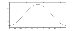
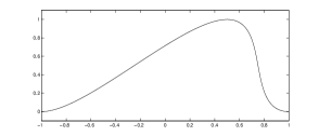
Fig. 1: Left smooth initial condition; right solution at $T=0.5$

N	$\|u-u_{h}\|_{L^{1}(I)}$	$\|u-u_{h}\|_{L^{2}(I)}$	$|\|\tilde{e}\||_{1}$ $(\sim H^{-1}(I))$	$|\|\tilde{e}\||_{h}$ $(\sim L^{2}(I))$
100	$2.5\cdot 10^{-3}$	$3.6\cdot 10^{-3}$	$3.0\cdot 10^{-4}$	$3.2\cdot 10^{-3}$
200	$6.7\cdot 10^{-4}$ (1.9)	$1.0\cdot 10^{-3}$ (1.8)	$7.0\cdot 10^{-5}$ (2.1)	$9.5\cdot 10^{-4}$ (1.8)
400	$1.8\cdot 10^{-4}$ (1.9)	$3.0\cdot 10^{-4}$ (1.7)	$1.7\cdot 10^{-5}$ (2.0)	$2.9\cdot 10^{-5}$ (1.7)
800	$4.6\cdot 10^{-5}$ (2.0)	$8.9\cdot 10^{-5}$ (1.8)	$4.2\cdot 10^{-6}$ (2.0)	$8.7\cdot 10^{-6}$ (1.7)

Table 1: $\epsilon=O(10^{-16})$, smooth solution

N	$\|u-u_{h}\|_{L^{1}(I)}$	$\|u-u_{h}\|_{L^{2}(I)}$	$|\|\tilde{e}\||_{1}$ $(\sim H^{-1}(I))$	$|\|\tilde{e}\||_{h}$ $(\sim L^{2}(I))$
100	$1.9\cdot 10^{-3}$	$3.0\cdot 10^{-3}$	$2.3\cdot 10^{-4}$	$2.6\cdot 10^{-3}$
200	$4.7\cdot 10^{-4}$ (2.0)	$7.7\cdot 10^{-4}$ (2.0)	$5.5\cdot 10^{-5}$ (2.1)	$7.1\cdot 10^{-4}$ (1.9)
400	$1.2\cdot 10^{-4}$ (2.0)	$2.1\cdot 10^{-4}$ (1.9)	$1.3\cdot 10^{-5}$ (2.1)	$1.9\cdot 10^{-4}$ (1.8)
800	$3.0\cdot 10^{-5}$ (2.0)	$5.5\cdot 10^{-5}$ (1.9)	$3.3\cdot 10^{-6}$ (2.0)	$5.3\cdot 10^{-5}$ (1.8)

Table 2: $\epsilon=h$, smooth solution

Now we consider a problem with non-smooth solution. The initial data and final time exact solution is given in Figure 2. We compute the solution at $T=0.5$ when the shock has formed. The exact solution is computed using the method of characteristics on a mesh with 12800 elements. We present tables with the same errors as in the previous case for the method without (Table 3) and with (Table 4) regularization. For this case there is even less difference between the two cases. We observe first order convergence for the $L^{1}$-error and the $H^{-1}$-norm error and $1/2$-order convergence in the $L^{2}$-norm. The computations clearly show how the weaker norm behaves either as an $L^{1}$-norm for $\delta=1$ or an $L^{2}$-norm for $\delta=h$. Intermediate values of $\delta$ appears to interpolate between these two norms. This indicates that the principle of our estimate, with the order depending on how $\delta$ is chosen with respect to $h$ is correct. A superconvergence of approximately half an order is observed for all the computations with the nonsmooth solution, compared to what is predicted by theory.

Fig. 2: Left nonsmooth initial condition; right solution at $T=0.5$

N	$\|u-u_{h}\|_{L^{1}(I)}$	$\|u-u_{h}\|_{L^{2}(I)}$	$|\|\tilde{e}\||_{1}$ $(\sim H^{-1}(I))$	$|\|\tilde{e}\||_{h}$ $(\sim L^{2}(I))$
100	$0.036$	$0.071$	$6.4\cdot 10^{-3}$	$0.038$
200	$0.018$ (1.0)	$0.049$ (0.5)	$3.2\cdot 10^{-3}$ (1.0)	$0.024$ (0.7)
400	$9.4\cdot 10^{-3}$ (0.9)	$0.034$ (0.5)	$1.6\cdot 10^{-3}$ (1.0)	$0.016$ (0.6)
800	$4.7\cdot 10^{-3}$ (1.0)	$0.023$ (0.6)	$7.9\cdot 10^{-4}$ (1.0)	$0.011$ (0.5)

Table 3: $\epsilon=O(10^{-16})$, nonsmooth solution

N	$\|u-u_{h}\|_{L^{1}(I)}$	$\|u-u_{h}\|_{L^{2}(I)}$	$|\|\tilde{e}\||_{1}$ $(\sim H^{-1}(I))$	$|\|\tilde{e}\||_{h}$ $(\sim L^{2}(I))$
100	$0.035$	$0.070$	$6.3\cdot 10^{-3}$	$0.037$
200	$0.018$ (1.0)	$0.048$ (0.5)	$3.2\cdot 10^{-3}$ (1.0)	$0.024$ (0.6)
400	$9.1\cdot 10^{-3}$ (1.0)	$0.033$ (0.5)	$1.6\cdot 10^{-3}$ (1.0)	$0.016$ (0.6)
800	$4.6\cdot 10^{-3}$ (1.0)	$0.023$ (0.5)	$7.9\cdot 10^{-4}$ (1.0)	$0.010$ (0.7)

Table 4: $\epsilon=h$, nonsmooth solution

References

- [1] A. Bonito, J.-L. Guermond, B. Popov. Stability analysis of explicit entropy viscosity methods for non-linear scalar conservation equations Math. Comp. published online 2013.
- [2] E. Burman. Adaptive finite element methods for compressible two-phase flows. PhD thesis, Chalmers University of Technology, 1998.
- [3] E. Burman. A unified analysis for conforming and nonconforming stabilized finite element methods using interior penalty. SIAM J. Numer. Anal. 43, no. 5, 2012–2033 2005.
- [4] E. Burman. On nonlinear artificial viscosity, discrete maximum principle and hyperbolic conservation laws. BIT, 47(4):715–733, 2007.
- [5] E. Burman and A. Ern. Stabilized Galerkin approximation of convection-diffusion-reaction equations: discrete maximum principle and convergence. Math. Comp., 74(252):1637–1652 (electronic), 2005.
- [6] E. Burman and M. A. Fernández. Continuous interior penalty finite element method for the time-dependent Navier-Stokes equations: space discretization and convergence. Numer. Math., 107(1):39–77, 2007.
- [7] C. Chainais-Hillairet. Finite volume schemes for a nonlinear hyperbolic equation. Convergence towards the entropy solution and error estimate. M2AN Math. Model. Numer. Anal. 33, no. 1, 129–156, 1999.
- [8] B. Cockburn ; P. -A. Gremaud. A priori error estimates for numerical methods for scalar conservation laws. I. The general approach. Math. Comp. 65, no. 214, 533–573, 1996.
- [9] B. Cockburn ; P. -A. Gremaud. Error estimates for finite element methods for scalar conservation laws. SIAM J. Numer. Anal. 33, no. 2, 522–554, 1996.
- [10] B. Cockburn. Continuous dependence and error estimation for viscosity methods. Acta Numer. 12, 127–180, 2003.
- [11] C. Cockburn ; F. Coquel ; P. LeFloch. An error estimate for finite volume methods for multidimensional conservation laws. Math. Comp. 63, no. 207, 77–103 1994.
- [12] C. Cockburn ; F. Coquel ; P. LeFloch. Convergence of the finite volume method for multidimensional conservation laws. SIAM J. Numer. Anal. 32, no. 3, 687–705, 1995.
- [13] F. Coquel ; P. LeFloch. Convergence of finite difference schemes for conservation laws in several space dimensions: a general theory. SIAM J. Numer. Anal. 30, no. 3, 675–700, 1993.
- [14] M. G. Crandall ; A. Majda. Monotone difference approximations for scalar conservation laws. Math. Comp. 34, no. 149, 1–21, 1980.
- [15] L. Dieci and L. Lopez. Sliding motion in Filippov differential systems: theoretical results and a computational approach. SIAM J. Numer. Anal., 47(3):2023–2051, 2009.
- [16] B. Engquist ; S. Osher. One-sided difference approximations for nonlinear conservation laws. Math. Comp. 36, no. 154, 321–351, 1981.
- [17] S. Evje ; K. H. Karlsen. Monotone difference approximations of BV solutions to degenerate convection-diffusion equations. SIAM J. Numer. Anal. 37, no. 6, 1838–1860, 2000.
- [18] A. F. Filippov. Differential equations with discontinuous right-hand side. Mat. Sb. (N.S.), 51 (93):99–128, 1960.
- [19] J.-L. Guermond, R. Pasquetti, and B. Popov. Entropy viscosity method for nonlinear conservation laws. J. Comput. Phys., 230(11):4248–4267, 2011.
- [20] A. A. Himonas and G. Misiołek. Non-uniform dependence on initial data of solutions to the Euler equations of hydrodynamics. Comm. Math. Phys., 296(1):285–301, 2010.
- [21] P. Houston, J. A. Mackenzie, E. Süli, and G. Warnecke. A posteriori error analysis for numerical approximations of Friedrichs systems. Numer. Math., 82(3):433–470, 1999.
- [22] C. Johnson, U. Nävert, and J. Pitkäranta. Finite element methods for linear hyperbolic problems. Comput. Methods Appl. Mech. Engrg., 45(1-3):285–312, 1984.
- [23] C. Johnson and A. Szepessy. On the convergence of a finite element method for a nonlinear hyperbolic conservation law. Math. Comp., 49(180):427–444, 1987.
- [24] C. Johnson and A. Szepessy. Adaptive finite element methods for conservation laws based on a posteriori error estimates. Comm. Pure Appl. Math. 48, no. 3, 199–234, 1995.
- [25] S. N. Krushkov The method of finite differences for a nonlinear equation of the first order with several independent variables. (Russian) Z. Vycisl. Mat. i Mat. Fiz. 6 884–894, 1966.
- [26] D. Kuzmin and S. Turek. Flux correction tools for finite elements. J. Comput. Phys., 175(2):525–558, 2002.
- [27] N. N. Kuznetsov. The accuracy of certain approximate methods for the computation of weak solutions of a first order quasilinear equation. Z. Vycisl. Mat. i Mat. Fiz. 16, no. 6, 1489–1502, 1976.
- [28] P. G. LeFloch. Hyperbolic systems of conservation laws. Lectures in Mathematics ETH Zürich. Birkhäuser Verlag, Basel, 2002. The theory of classical and nonclassical shock waves.
- [29] H. Nessyahu ; E. Tadmor. The convergence rate of approximate solutions for nonlinear scalar conservation laws. SIAM J. Numer. Anal. 29, no. 6, 1505–1519, 1992.
- [30] M. Ohlberger. A posteriori error estimate for finite volume approximations to singularly perturbed nonlinear convection-diffusion equations. Numer. Math. 87, no. 4, 737–761, 2001.
- [31] O. A. Oleinik. Discontinuous solutions of non-linear differential equations. Amer. Math. Soc. Transl. (2) 26 95–172, 1963 (Russian original in Uspehi Mat. Nauk (N.S.) 12 1957 no. 3(75), 3–73.)
- [32] E. Tadmor. Approximate solutions of nonlinear conservation laws. in Advanced Numerical Approximation of Nonlinear Hyperbolic Equations (A. Quarteroni, ed.), Vol. 1697 of Lecture Notes in Mathematics: Subseries Fondazione C.I.M.E., Firenze, Springer, pp. 1–149, 1998.
- [33] J. Xu and L. Zikatanov. A monotone finite element scheme for convection-diffusion equations. Math. Comp., 68(228):1429–1446, 1999.