Testing Cosmology with Extreme Galaxy Clusters

Abstract

Motivated by recent suggestions that a number of observed galaxy clusters have masses which are too high for their given redshift to occur naturally in a standard model cosmology, we use Extreme Value Statistics to construct confidence regions in the mass-redshift plane for the most extreme objects expected in the universe. We show how such a diagram not only provides a way of potentially ruling out the concordance cosmology, but also allows us to differentiate between alternative models of enhanced structure formation. We compare our theoretical prediction with observations, placing currently observed high and low redshift clusters on a mass-redshift diagram and find – provided we consider the full sky to avoid a posteriori selection effects – that none are in significant tension with concordance cosmology.

1 Introduction

In the standard “concordance” ($\Lambda$CDM) model of cosmology, structure formation proceeds in a hierarchical, ‘bottom-up’ fashion, with small scale perturbations in the initial distribution of Cold Dark Matter (CDM) collapsing first, before merging over time to form larger and larger haloes. The initial, nearly Gaussian, distribution of these overdensities means that large fluctuations, and correspondingly large halo masses, should be extremely rare in the early universe. However, many of the plausible extensions to the concordance model have been found to be capable of enhancing (or depleting) structure formation, including primordial non-Gaussianity (Lucchin & Matarrese, 1988; Pillepich et al., 2010), modified gravity (Schmidt et al., 2009; Ferraro et al., 2011) and scalar field (Baldi & Pettorino, 2011; Mortonson et al., 2011; Tarrant et al., 2011) scenarios. Furthermore, each of these extensions can affect structure formation in different ways at different times in the history of the universe, meaning that if we can construct a history of the growth of structure we can discriminate between competing models.

In addition, much attention has recently been paid to the prospect that the existence of a single extreme (in terms of its high mass and redshift) object in the universe has the potential to rule out at a high significance level cosmological models in which it is correspondingly unlikely to exist. Following observations of a series of apparently extreme objects (Jee et al., 2009; Brodwin et al., 2010; Foley et al., 2011; Menanteau et al., 2011; Planck Collaboration et al., 2011; Santos et al., 2011), some authors have claimed that such objects are either highly unlikely to exist (Jimenez & Verde, 2009; Holz & Perlmutter, 2010; Cayón et al., 2011; Hoyle et al., 2011) in a concordance $\Lambda$CDM cosmology or, more powerfully, are significantly larger than the expected most massive object in a $\Lambda$CDM universe (Chongchitnan & Silk, 2011), although Waizmann et al. (2011a) contend this result. As well as highlighting tensions with the standard model, various authors have shown how such high-mass, high-redshift objects may be explained by an enhanced rate of structure formation generated by the inclusion of primordial non-Gaussianity (Enqvist et al., 2011; Hoyle et al., 2011; Cayón et al., 2011; Chongchitnan & Silk, 2011) or scalar field dark energy (Waizmann et al., 2011b) into the concordance cosmology.

In this paper we build on our previous work using extreme value statistics (Harrison & Coles, 2011) to test the current concordance model with extreme galaxy clusters as well investigating the different behaviours of extreme clusters in alternative models. We construct the probability contours of the highest mass cluster for all redshifts in an observational survey and directly compare the current best fit $\Lambda$CDM model with observations showing that, if we consider the full sky (in order to avoid a posteriori selection effects) then none of the currently observed extreme galaxy clusters are in tension with the $\Lambda$CDM model. Then, using information from the CoDECS (Baldi, 2011a) N-body simulations, we show how, if any future observations do exclude the $\Lambda$CDM model, extreme clusters can potentially be used to understand which of the alternative models available may best explain the enhanced structure formation.

The paper is organised as follows. In section 2 we introduce extreme value statistics and show how they may be used to predict the mass of the most extreme cluster within an observational survey. Section 3 compares predictions for a $\Lambda$CDM universe with observations. Section 4 shows how the plot of extreme value contours against redshift can highlight differences between cosmological models. In section 5 we conclude and discuss prospects for future work in this area.

2 Method

Extreme Value Statistics (EVS) (Gumbel, 1958; Katz & Nadarajah, 2002) seeks to make predictions for the properties of the greatest (or least) valued random variable drawn from an underlying distribution. If we consider a sequence of $N$ random variates $\{M_{i}\}$ drawn from a cumulative distribution $F(m)$ then there will be a largest value of the sequence: $M_{\rm max}\equiv\sup\{M_{1},\ldots M_{N}\}.$ If these variables are mutually independent and identically distributed then the probability that all of the deviates are less than or equal to some $m$ is given by:

$$\Phi(M_{\rm max}\leq m;N) = F_{1}(M_{1}\leq m)\ldots F_{N}(M_{N}\leq m)$$ (1)

$$= F^{N}(m)$$

and the probability density function (pdf) for $M_{\rm max}$ is then found by differentiating (1):

$$\phi(M_{\rm max}=m;N)=Nf(m)\left[F(m)\right]^{N-1},$$ (2)

where $f(m)=dF(m)/dm$ is the pdf of the original distribution. This gives the exact extreme value pdf for $N$ observations drawn from a known distribution $F(m)$; for more discussion of the advantages of this approach over others involving the use of asymptotic theory, see
citeHarrison2011. To apply this general result to the concrete example of the most massive cluster we use the appropriate halo mass function, which gives the number density of haloes $n(M)$, to derive $f(m)$ and $F(m)$ according to:

$$f(m) = \frac{1}{n_{\rm tot}}\frac{dn(m)}{dm},$$ (3)

$$F(m) = \frac{1}{n_{\rm tot}}\left[\int_{-\infty}^{m}dM\,\frac{dn(M)}{dM}\right],$$ (4)

where the normalisation factor

$$n_{\rm tot}=\int_{-\infty}^{\infty}dM\,\frac{dn(M)}{dM}$$ (5)

is the total (co-moving) number density of haloes. For a constant redshift box of volume $V$ the total number of expected haloes $N$ is given by $n_{\rm tot}V$. These distributions can be inserted into equation (2) to predict the pdf of the highest mass dark matter halo within the volume. Although this procedure explicitly assumes that haloes are uncorrelated, we have found (Harrison & Coles, 2011) that the results closely match those of Davis et al. (2011), who construct their extreme value distribution as the differential of the void probability:

$$\Phi^{\rm void}(M_{\rm max}=m)=\frac{dP_{0}(m)}{dm},$$ (6)

(allowing them to account for complications due to halo correlations and bias), for the high masses of relevance to the inference we are interested in.

In a cosmological survey we observe clusters at various redshifts along our past light cone rather than on a single spatial hypersurface at fixed $z$. If we wish to construct the EVS for galaxy clusters within an observational survey which covers a fraction $f_{\rm sky}$ of the sky between redshifts $z_{\rm min}$ and $z_{\rm max}$ we therefore need to take into account both the effect of the growth of structure with decreasing redshift on the halo mass function $n(m,z)$ and the observational volume we are probing in an expanding universe, via the volume element $dV/dz$. Doing this allows us to form the pdf of halo masses within that survey as:

$$f(m) = \frac{f_{\rm sky}}{N_{tot}}\left[\int^{z_{\rm max}}_{z_{min}}dz\,\frac{dV}{dz}\frac{dn(m,z)}{dm}\right],$$ (7)

$$F(m) = \frac{f_{\rm sky}}{N_{tot}}\left[\int^{z_{\rm max}}_{z_{min}}\int^{m}_{-\infty}dz\,dM\,\frac{dV}{dz}\frac{dn(M,z)}{dM}\right],$$ (8)

where

$$N_{tot} = f_{\rm sky}\left[\int^{z_{\rm max}}_{z_{min}}\int^{\infty}_{-\infty}dz\,dM\,\frac{dV}{dz}\frac{dn(M,z)}{dM}\right].$$ (9)

and then feed these distributions into our extreme value prescription (2) (of course it is impractical to integrate numerically to infinite endpoints and so finite limits of $12<\log_{10}m<18$ are chosen; we have checked that this choice makes no difference to the conclusions). In order to make best use of this information, we want to be able to see the distributions for all redshifts at once; we hence construct the EVS distribution for narrow bins in redshift space $\Delta z=0.02$ (chosen so that $N_{bins}>>N_{clusters}$ and the highest expected mass for all redshifts remains the same as for $N_{bins}=1$), integrate over these pdfs to find the $66\%,95\%$ and $99\%$ confidence regions and plot these, along with the peak of the distribution, for all redshifts $0<z<2$. This can then be used to test the cosmological model: if an observed cluster lies above e.g. the $95\%$ region of such a distribution, then we may say we have a correspondingly significant detection of enhanced structure formation at that redshift.

3 Comparison with Observations

We can now apply this technique to find out if any currently observed clusters are discordant with the concordance $\Lambda$CDM predictions. We emphasize that, because we are predicting the distributions of the most massive cluster at each redshift, if even a single galaxy cluster lying outside the extreme value contours when placed on a mass-redshift plot can be seen as a significant detection of deviation from concordance cosmology.

3.1 Calibration of Cosmology and Cluster Masses

Cluster	$z$	$M_{200\rm m}^{\rm Edd}/M_{\odot}$
A21631	$0.203$	$3.04_{-0.67}^{+0.87}\times 10^{15}$
A3701	$0.375$	$2.62_{-0.67}^{+0.87}\times 10^{15}$
RXJ13471	$0.451$	$2.14_{-0.48}^{+0.60}\times 10^{15}$
ACT-CL J01022	$0.87$	$1.85_{-0.33}^{+0.42}\times 10^{15}$
PLCK G2663	$0.94$	$1.45^{+0.27}_{-0.20}\times 10^{15}$
SPT-CL J21064	$1.132$	$1.11_{-0.20}^{+0.24}\times 10^{15}$
SPT-CL J05465	$1.067$	$7.80^{+1.27}_{-0.90}\times 10^{14}$
XXMU J22356	$1.4$	$6.82_{-1.23}^{+1.52}\times 10^{14}$
XXMU J00447	$1.579$	$4.02_{-0.73}^{+0.88}\times 10^{14}$

Table 1: The extreme clusters considered in this paper ([1] Maughan et al. 2011, [2] Menanteau et al. 2011, [3]Planck Collaboration et al. 2011, [4] Foley et al. 2011, [5] Brodwin et al. 2010, [6] Jee et al. 2009, [7] Santos et al. 2011). $M_{200\rm m}^{\rm Edd}$ is calculated using the numerical code of (Zhao et al., 2009) to convert from $M_{200\rm c}$ (where necessary) and equation (12) to include the Eddington bias.

In order to meaningfully compare our theoretical predictions to observations, we need to carefully ensure our $\Lambda$CDM cosmology is correctly calibrated. As the ingredients for our concordance cosmology here, we use a linear matter power spectrum $P(k)$ calculated using the numerical code CAMB and the WMAP7+BAO+H0 Mean parameters from Komatsu et al. (2011). From this we calculate the variance of the matter field, smoothed with a top hat window $W(k;R)$ of radius $R=(3m/4\pi\bar{\rho}_{m,0})^{1/3}$, evolved to a redshift $z$ with the linear growth function $D_{+}(z)$ (normalised to $D_{+}(0)=1$):

$$\sigma^{2}(m,z)=D_{+}^{2}(z)\int_{0}^{\infty}\frac{dk}{2\pi}\,k^{2}P(k)W^{2}(k;R).$$ (10)

This is used as the input for the halo mass function from Tinker et al. (2008):

$$\frac{dn(m,z)}{dm}=A\left[\left(\frac{\sigma}{b}\right)^{-a}+1\right]e^{-c/\sigma^{2}}\frac{\bar{\rho}_{m,0}}{m}\frac{d\mathrm{ln}(\sigma^{-1})}{dm}.$$ (11)

where $\bar{\rho}_{m,0}$ is the mean density in the universe at redshift $z=0$, $\delta_{c}\simeq 1.686$ is the critical overdensity for collapse and $\{A,a,b,c\}$ are given the values for $m_{200m}$ (the mass corresponding to the portion of the cluster which has density greater than $200\bar{\rho}_{m,0}$) from Tinker et al. (2008) of $\{0.186,1.47,2.57,1.19\}$.

When comparing to real-world clusters we need to correct for the fact that theoretical mass functions are defined with respect to the average matter density $\bar{\rho}_{m,z}$, but observers frequently report cluster masses with respect to the critical density $\rho_{c}$. In order to do this, we follow the procedures of Waizmann et al. (2011a) and Mortonson et al. (2011) to convert all cluster masses to $m_{200m}$, and correct for Eddington bias. Eddington bias refers to the fact that there is a larger population of small mass haloes which may up-scatter into our observations than there are high mass haloes which may down-scatter into them, and is corrected for using:

$$\ln m^{Edd}=\ln m+\frac{1}{2}\epsilon\sigma_{\ln m}^{2},$$ (12)

where $\epsilon$ is the local slope of the halo mass function and $\sigma_{\ln m}^{2}$ is the measurement uncertainty for the cluster mass.

In order to ensure we are avoiding a posteriori selection (by only performing our test in regions in which we have already observed something which we believe to be unusual) we set $f_{sky}=1$. This is both the most conservative estimate and, we believe, the correct one for testing ‘the most extreme clusters in the sky’.

3.2 Results

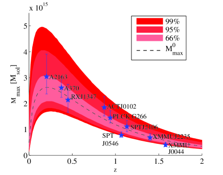
Figure 1: Extreme value contours and modal highest-mass cluster with redshift for a $\Lambda$CDM cosmology, along with a set of currently observed ‘extreme’ galaxy clusters. None lie in the region above the $99\%$ contour and hence are consistent with

a concordance cosmology.

We now seek to use the apparatus described above to test if any currently observed objects are significantly extreme to give us cause to question $\Lambda$CDM cosmology. We consider the set of recently observed, potentially extreme clusters shown in table 1 in a $\Lambda$CDM cosmology as described above. The extreme value contours (light - $99\%$, medium - $95\%$, dark - $66\%$), most likely maximum mass ${M}^{0}_{\rm max}$ (solid line) and the cluster masses and redshifts (stars) are plotted in Figure 1. The plot shows the expected features of a peak in maximum halo mass at $z\approx 0.2$ (the location and height of which is in broad agreement with the analysis of Holz & Perlmutter 2010). As can be seen, none of the currently observed clusters lie outside the $99\%$ confidence regions of the plot meaning that there is no current strong evidence for a need to modify the $\Lambda$CDM concordance model from high-mass high-redshift clusters. This appears to be in agreement with the findings of Waizmann et al. (2011a) for a similar set of clusters, but in contradiction to Chongchitnan & Silk (2011) who find that the cluster XMMUJ0044 is a $4\sigma$ result (i.e. should lie well above the $99\%$ region in Figure 1), whilst here we find it to be well within the acceptable region.

4 Testing Cosmological Models with Extreme Clusters

In addition to simply ruling out $\Lambda$CDM cosmology with massive clusters, we may also consider whether extreme objects offer the potential to discriminate between different alternative models. Whilst many alternative models are capable of predicting enhanced structure formation, the exact scale and time dependence of the enhancement will differ from model to model. Here we consider two models which have a well defined and investigated effect on the halo mass function, and hence are relatively simple to calculate the extreme value statistics over a range of redshift for: local form primordial non-Gaussianity and the bouncing, coupled scalar field dark energy model labelled as ‘SUGRA003’ in Baldi (2011b). These should be regarded as toy models – our aim is to show how the extreme value statistics can be used to select between different models, rather than make definite predictions.

4.1 Models Considered

We make use of the CoDECS simulations kindly made publicly available by Baldi et al. (2010); Baldi (2011a). This suite of large N-body simulations includes realisations of both $\Lambda$CDM and a number of coupled dark energy cosmologies. Here, we compare the CoDECS $\Lambda$CDM-L (where ‘L’ is for ‘Large’) simulation of the concordance cosmology to both the primordial non-Gaussianity and the SUGRA003 (supergravity) bouncing dark energy models. Primordial non-Gaussianity, motivated by considerations of the fluctuations of the inflaton field, is one of the most widely explored modifications to the concordance cosmology (e.g. Desjacques & Seljak, 2010) and has long (Lucchin & Matarrese, 1988) been known to affect the abundances of high-mass galaxy clusters. It has also been the model most invoked (Jimenez & Verde, 2009; Cayón et al., 2011; Chongchitnan & Silk, 2011; Hoyle et al., 2011) to account for apparently over-massive high redshift objects, all of these authors reporting values of local non-Gaussianity parameter $f_{NL}\sim 300-500$ as being able to account for such clusters.

However, Baldi (2011b) points out that such models enhance numbers of high mass clusters at all redshifts, creating tension with observations at low redshift in the attempt to alleviate them at high redshift. As an alternative scenario, the supergravity-motivated scalar field scenario of Brax & Martin (1999) is considered. This model includes a scalar field component $\phi$ which couples to dark matter with a coupling strength $\beta$ and has the self interacting potential:

$$V(\phi)=B\phi^{-\alpha}e^{\phi^{2}/2}$$ (13)

This scalar field component acts as a ‘bouncing’ dark energy; structure formation is enhanced at early times, but is suppressed with respect to $\Lambda$CDM after the point at which the evolution of $\phi$ changes sign (the ‘bounce’), meaning $\Lambda$CDM values for $\sigma_{8}$ can still be reproduced at $z=0$. In order to match background observables given by WMAP7 constraints (Komatsu et al., 2011), the SUGRA003 version of the potential has ‘tuned’ parameters $\{B,\alpha,\beta\}=\{0.0202,2.15,-0.15\}$.

For $\Lambda$CDM and SUGRA models, we fit a halo mass function of the Tinker et al. (2008) form directly to the haloes identified using a friends-of-friends (FoF) algorithm with linking length $l=0.2\bar{d}$ (where $\bar{d}$ is the mean inter-particle separation) in the relevant CoDECS simulation ($\Lambda$CDM-L and SUGRA003-L respectively). For the primordial non-Gaussianity model, we apply a non-Gaussian correction factor $\mathcal{R}(f_{\rm NL})$ to the halo mass functions found in the $\Lambda$CDM-L simulation, choosing the $\mathcal{R}(f_{\rm NL})$ of Lo Verde et al. (2008) (LMSV):

$$\mathcal{R}_{LMSV}(f_{NL})=$$ (14)

$$1+\frac{\sigma^{2}}{6\delta_{c}}\left[S_{3}(\sigma)\left(\frac{\delta_{c}^{4}}{\sigma^{4}}-\frac{2\delta_{c}^{2}}{\sigma^{2}}-1\right)+\frac{dS_{3}}{d\ln\sigma}\left(\frac{\delta_{c}^{2}}{\sigma^{2}}-1\right)\right].$$

where $S_{3}$ is the normalised skewness of the matter density field, for which we use the approximation:

$$S_{3}\simeq 3\times 10^{-4}f_{NL}\sigma^{-1}$$ (15)

given by equation (2.7) of Enqvist et al. (2011). We adopt a value of $f_{NL}=300$ for our non-Gaussian model as it is both consistent with the observational findings discussed above and leads to a similar magnitude of enhancement of structure formation at high redshifts as the SUGRA003 model.

The values of $H(z)$ and $D_{+}(z)$ required to find $dV/dz$ for all three models are calculated using the tabulated growth functions and expansion histories for the cosmologies, numerically calculated from the evolution equations and provided on the CoDECS website.

4.2 Results

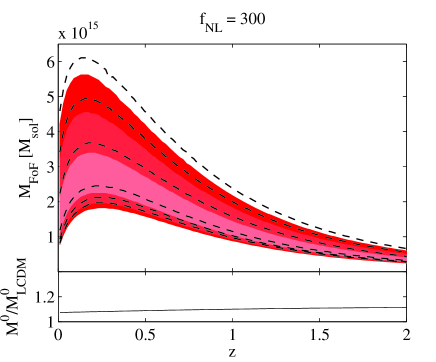
Figure 2: Extreme value contours for $\Lambda$CDM (shaded regions), $f_{NL}$ and SUGRA models (dashed lines). Lower plots are the enhancement of modal highest-mass cluster over the $\Lambda$CDM value, showing different behaviour for the two alternative models.

With the halo mass functions and expansion histories of each cosmology we are then able to carry out the procedure of section 2 to find the EVS of objects within an observational survey in each cosmology, the results of which are shown in Figure 2. Plotted are extreme value contours (light - $99\%$, medium - $95\%$, dark - $66\%$) for the $\Lambda$CDM model and the edges of the three extreme value contours for the non-Gaussian and SUGRA models (dashed lines) as well as the enhancement in the most likely maximum mass $M^{0}_{\rm max}$ over the $\Lambda$CDM predictions. As can be seen (and as expected) the primordial non-Gaussianity model shows an enhancement of the mass of the highest mass cluster at all redshifts, whilst the SUGRA model is capable of enhancing $M^{0}_{\rm max}$ at high redshifts whilst leaving it unchanged at more recent times. Thus, if $\Lambda$CDM is ruled out by both high and low redshift clusters, primordial non-Gaussianity could be seen as the favoured explanation whilst, if only high redshift observations appear in contradiction, both non-Gaussian and SUGRA models would be allowed (unless the limit of an ideal, complete survey was reached).

5 Discussion and Conclusions

In this paper we have presented a theoretical framework for the interpretation of extremely massive clusters in cosmological surveys. We avoid ambiguities in the volume being probed by observed clusters which occur in the alternative approach of using single clusters to estimate the halo mass function $n(m)$. Our method, in contrast, does not require such normalisation and is both more robust and, inevitably, more conservative, a combination of attributes which we believe should best describe confrontations of theory with observations.

We have used this method to show that existing observations of extreme clusters are not incompatible with the predictions of $\Lambda$CDM concordance cosmology. However in anticipation of future, more complete surveys, we have also presented a definitive calculation of the region in the mass-redshift plane in which the presence of a single cluster would exclude the standard model with high confidence. We have also shown that different cosmological models including physics beyond the concordance picture are capable of making significantly different predictions of the allowable regions in the mass-redshift plane. This means that whilst current extreme cluster data do not discriminate between the $\Lambda$CDM model and these alternatives, future data may well be capable of doing so. We intend in due course to extend the approach presented here by incorporating it into a full model selection analysis.

References

- Baldi (2011a) Baldi, M., 2011a, ArXiv e-prints, arXiv:1109.5695
- Baldi (2011b) Baldi, M., 2011b, ArXiv e-prints, arXiv:1107.5049
- Baldi & Pettorino (2011) Baldi, M., Pettorino, V., 2011, MNRAS, 412, L1, arXiv:1006.3761
- Baldi et al. (2010) Baldi, M., Pettorino, V., Robbers, G., Springel, V., 2010, MNRAS, 403, 1684, arXiv:0812.3901
- Brax & Martin (1999) Brax, P. H., Martin, J., 1999, Physics Letters B, 468, 40, arXiv:astro-ph/9905040
- Brodwin et al. (2010) Brodwin, M., Ruel, J., Ade, P. A. R., et al., 2010, ApJ, 721, 90, arXiv:1006.5639
- Cayón et al. (2011) Cayón, L., Gordon, C., Silk, J., 2011, MNRAS, 415, 849, arXiv:1006.1950
- Chongchitnan & Silk (2011) Chongchitnan, S., Silk, J., 2011, ArXiv e-prints, arXiv:1107.5617
- Davis et al. (2011) Davis, O., Devriendt, J., Colombi, S., Silk, J., Pichon, C., 2011, MNRAS, 413, 2087, arXiv:1101.2896
- Desjacques & Seljak (2010) Desjacques, V., Seljak, U., 2010, Classical and Quantum Gravity, 27, 12, 124011, arXiv:1003.5020
- Enqvist et al. (2011) Enqvist, K., Hotchkiss, S., Taanila, O., 2011, J. Cosmology Astropart. Phys, 4, 17, arXiv:1012.2732
- Ferraro et al. (2011) Ferraro, S., Schmidt, F., Hu, W., 2011, Phys. Rev. D, 83, 6, 063503, arXiv:1011.0992
- Foley et al. (2011) Foley, R. J., Andersson, K., Bazin, G., et al., 2011, ApJ, 731, 86, arXiv:1101.1286
- Gumbel (1958) Gumbel, E. J., 1958, Statistics of Extremes, Columbia University Press
- Harrison & Coles (2011) Harrison, I., Coles, P., 2011, MNRAS, 418, L20, arXiv:1108.1358
- Holz & Perlmutter (2010) Holz, D. E., Perlmutter, S., 2010, ArXiv e-prints, arXiv:1004.5349
- Hoyle et al. (2011) Hoyle, B., Jimenez, R., Verde, L., 2011, Phys. Rev. D, 83, 10, 103502, arXiv:1009.3884
- Jee et al. (2009) Jee, M. J., Rosati, P., Ford, H. C., et al., 2009, ApJ, 704, 672, arXiv:0908.3897
- Jimenez & Verde (2009) Jimenez, R., Verde, L., 2009, Phys. Rev. D, 80, 12, 127302, arXiv:0909.0403
- Katz & Nadarajah (2002) Katz, S., Nadarajah, S., 2002, Extreme Value Distributions, Theory and Applications, Imperial College Press
- Komatsu et al. (2011) Komatsu, E., Smith, K. M., Dunkley, J., et al., 2011, ApJS, 192, 18, arXiv:1001.4538
- Lo Verde et al. (2008) Lo Verde, M., Miller, A., Shandera, S., Verde, L., 2008, J. Cosmology Astropart. Phys, 4, 14, arXiv:0711.4126
- Lucchin & Matarrese (1988) Lucchin, F., Matarrese, S., 1988, ApJ, 330, 535
- Maughan et al. (2011) Maughan, B. J., Giles, P. A., Randall, S. W., Jones, C., Forman, W. R., 2011, ArXiv e-prints, arXiv:1108.1200
- Menanteau et al. (2011) Menanteau, F., Hughes, J. P., Sifon, C., et al., 2011, ArXiv e-prints, arXiv:1109.0953
- Mortonson et al. (2011) Mortonson, M. J., Hu, W., Huterer, D., 2011, Phys. Rev. D, 83, 2, 023015, arXiv:1011.0004
- Pillepich et al. (2010) Pillepich, A., Porciani, C., Hahn, O., 2010, MNRAS, 402, 191, arXiv:0811.4176
- Planck Collaboration et al. (2011) Planck Collaboration, Aghanim, N., Arnaud, M., et al., 2011, ArXiv e-prints, arXiv:1106.1376
- Santos et al. (2011) Santos, J. S., Fassbender, R., Nastasi, A., et al., 2011, A&A, 531, L15, arXiv:1105.5877
- Schmidt et al. (2009) Schmidt, F., Lima, M., Oyaizu, H., Hu, W., 2009, Phys. Rev. D, 79, 8, 083518, arXiv:0812.0545
- Tarrant et al. (2011) Tarrant, E. R. M., van de Bruck, C., Copeland, E. J., Green, A. M., 2011, ArXiv e-prints, arXiv:1103.0694
- Tinker et al. (2008) Tinker, J., Kravtsov, A. V., Klypin, A., et al., 2008, ApJ, 688, 709, arXiv:0803.2706
- Waizmann et al. (2011a) Waizmann, J.-C., Ettori, S., Moscardini, L., 2011a, ArXiv e-prints, arXiv:1109.4820
- Waizmann et al. (2011b) Waizmann, J.-C., Ettori, S., Moscardini, L., 2011b, MNRAS, 418, 456, arXiv:1105.4099
- Zhao et al. (2009) Zhao, D. H., Jing, Y. P., Mo, H. J., Börner, G., 2009, ApJ, 707, 354, arXiv:0811.0828