Interstellar Communication: The Case for Spread Spectrum

Abstract

Spread spectrum, widely employed in modern digital wireless terrestrial radio systems, chooses a signal with a noise-like character and much higher bandwidth than necessary. This paper advocates spread spectrum modulation for interstellar communication, motivated by robust immunity to radio-frequency interference (RFI) of technological origin in the vicinity of the receiver while preserving full detection sensitivity in the presence of natural sources of noise. Receiver design for noise immunity alone provides no basis for choosing a signal with any specific character, therefore failing to reduce ambiguity. By adding RFI to noise immunity as a design objective, the conjunction of choice of signal (by the transmitter) together with optimum detection for noise immunity (in the receiver) leads through simple probabilistic argument to the conclusion that the signal should possess the statistical properties of a burst of white noise, and also have a large time-bandwidth product. Thus spread spectrum also provides an implicit coordination between transmitter and receiver by reducing the ambiguity as to the signal character. This strategy requires the receiver to guess the specific noise-like signal, and it is contended that this is feasible if an appropriate pseudorandom signal is generated algorithmically. For example, conceptually simple algorithms like the binary expansion of common irrational numbers like $\pi$ are shown to be suitable. Due to its deliberately wider bandwidth, spread spectrum is more susceptible to dispersion and distortion in propagation through the interstellar medium, desirably reducing ambiguity in parameters like bandwidth and carrier frequency. This suggests a promising new direction in interstellar communication using spread spectrum modulation techniques.

1 INTRODUCTION

This paper addresses the design of an end-to-end digital interstellar communication system that can be used to exchange information among intelligent civilizations. As advocated in [1], we employ communication’s engineering principles to achieve an implicit form of coordination. This strategy leverages the physical impairments that are unavoidable in an end-to-end interstellar digital communication system, and presumably known to both transmitter and receiver, and bases design decisions on mitigation of those impairments. Where those design decisions are based on mathematical optimization, the transmitter and receiver designers will necessarily arrive at compatible designs. Where optimization is not possible, the receiver must apply judgement and/or systematically search over the possibilities, minimizing ambiguity by keeping the design as simple as possible within the constraints of acceptable cost and performance.

There are two distinct phases to establishing information transfer [1]: (a) receiver discovery of the existence of a signal followed by (b) extraction of information from that signal. This is rendered more challenging by the impossibility of advance coordination between transmitter and receiver, and discovery is the more challenging problem and also represents the dominant cost and effort for a receiving civilization. Although this paper addresses both discovery and communication from an end-to-end perspective, past efforts have addressed transmission and reception as primarily separate issues, and in the case of the receiver (with the exception of [2, 3]) have focused on discovery of signals designed to attract attention but not bear information. Some entryways into the extensive literature on this topic can be found in [4, 5, 6, 7, 8, 9]. Longstanding programs try to discover signals of technological origin [10] (called “SETI” [4]). Other efforts have transmitted signals with an embedded message (called “METI” [11]), including the “Arecibo message” [12] in 1974 and more recently “Cosmic Call”, “Teen Age Message” and “A Message from Earth” [8]. The transmitter side has also been studied from a cost perspective [13, 14].

The end-to-end design of interstellar communication systems is relevant to both SETI and METI. Our focus is on radio frequencies, digital modulation (although analog modulation has also been experimented with [8] in METI), and communication of an information-bearing message [9]. Many SETI projects have followed the Cyclops Report [15] more than four decades ago, which recommended searching for extremely narrow bandwidth signals. Several factors have changed since then. First, the explosion in terrestrial wireless multi-user communications systems has improved our understanding of radio communications in an RFI-dominated environment [16, 17, 18]. This has strongly shifted the design of radio systems toward spread spectrum techniques, in which the signal bandwidth is much greater than dictated by the supported information rates [19, 20]. Second, there has been great progress in understanding the radio propagation properties of the interstellar medium (ISM) based in large part on pulsar astronomy [21]. Third, dramatic advances in electronics technology open up new possibilities in our own search capabilities.

Here we consider the specific design criterion of maximizing the probability of discovering an information-bearing signal and the correct detection of its embedded information content. This criterion is appropriate for a transmitter constrained in transmit power and seeking to maximize the distance over which a message signal can be discovered and its information content extracted. For a given transmit power this criterion also maximizes the number of stellar systems wherein discovery is feasible, and in this sense the probability that the signal will be discovered by someone somewhere. Even if the details of the transmit signal are completely known to the receiver, there are four primary impairments beyond the control of transmitter and receiver designers that impinge on discovery and detection: natural noise sources, radio-frequency interference (RFI) in the receiver vicinity, radio propagation effects [22] through the interstellar medium (ISM), and Doppler due to relative accelerations. This paper focuses on the first two, and subsequent papers (starting with [23]) will address the remaining.

RFI is a challenge for SETI because its technological origin mimics the interstellar signal being sought. An ongoing trend on earth and its immediate environs is ever-increasing local RFI. It is possible that a transmitter designer (which is likely to be more technologically mature than us) has experienced a similar growth in RFI and also has developed an understanding of RFI mitigation in the context of its own multi-user wireless communication systems. If so, the transmitter designer may view RFI mitigation in the receiver environment as a significant design objective. We demonstrate in this paper that this circumstance would be very fortunate, for two reasons. First, signal choice by the transmitter taking RFI into account can strongly mitigate the adverse effects of RFI on our own SETI observations, directly addressing our growing challenge. Second, considerations of signal acquisition in the presence of RFI allow us to infer very specific characteristics of an information-bearing signal, considerably beyond what design for noise (as pursued in [15] and elsewhere) can infer. This establishes principles allowing us to infer what type of signal may have been chosen by the transmitter. In contrast, even recent attempts at applying communication theory to SETI have emphasized noise sensitivity [24, 25, 26, 2, 27, 28], and are as a result unable to infer any concrete characteristics of the signal even as many advocate the use of greater bandwidth. The propagation characteristics of the ISM introduce further constraints on the bandwidth and carrier frequency of the transmit signal, which desirably limits the ambiguity in these parameters for both transmitter and receiver [23]. Others have emphasized such astrophysical effects in trying to infer signal characteristics [29].

The focus of this paper is on the choice of a transmitted signal, which directly parallels the receiver’s challenge of anticipating what type of signal to expect. In this we take the perspective of a transmitter designer, because in the absence of explicit coordination it is the transmitter, and the transmitter alone, that chooses the signal. This is significant because the transmitter designer possesses far less information about the receiver’s environment than the receiver designer, due to both distance (tens to hundreds of light-years) and speed-of-light delay (tens to hundreds of years). While the receiver design can and should take into account all relevant characteristics of its local environs and available resources and technology, in terms of the narrower issue of what type of signal to expect the receiver designer must rely exclusively on the perspective of the transmitter designer.

The primary result of this paper is as follows. The transmitter designer should assume that the receiver employes the optimum detection algorithm for white Gaussian noise, but assume nothing specific about the RFI environment of the receiver since nothing is presumably known. The transmitter can, however, explicitly design a transmit signal that minimizes the effect of RFI on the receiver’s discovery and detection probabilities in a robust way; that is, in a way that provides a constant immunity regardless of the nature of the RFI. It is shown that the resulting immunity increases with the product of time duration and bandwidth, and that the signal should resemble statistically a burst of white noise. Intuitively this is advantageous because RFI resembles such a signal with a likelihood that decreases exponentially with time-bandwidth product. Both a transmitter and receiver designer using this optimization criterion and employing the tools of elementary probability theory will arrive at this same conclusion. Although the context is different, variations on this principle inform the design of many modern widely deployed terrestrial digital wireless communication systems, so this has been extensively tested in practice and is likely to have a prominent place in the technology portfolio of an extraterrestrial civilization as well.

2 DESIGN APPROACH

This section qualitatively describes an end-to-end digital communication system including counteracting noise and RFI. Section 3 brings to bear a relevant mathematical principle drawn from probability theory.

2.1 Modulation

An intermediate step of modulation (A) accommodates the analog nature of a radio channel. A common case is pulse-amplitude modulation (PAM), in which a sequence of information-bearing symbols $\{A_{k}\}$ , each drawn from a finite constellation (finite set of discrete points), is used to adjust the amplitude of a sequence of pulses with shape $h(t)$,

$$y(t)=\sqrt{\mathcal{E}_{h}}\cdot\sum_{k}A_{k}\,h(t-kT)\,.$$ (1)

It is assumed that $h(t)$ is a unit-energy pulse waveform, $1/T$ is the symbol rate, and $\mathcal{E}_{h}$ is the energy per symbol. If the receiver can distinguish which $A_{k}$ was transmitted, it can extract the information being conveyed. The average power is $\mathcal{P}_{s}=\mathcal{E}_{s}/T$, and if it is desired to reduce $\mathcal{P}_{s}$ (at the expense of lower information rate) this can be done by increasing $T$. The radio propagation must be passband with some carrier frequency $f_{c}$, and as described in A this allows the baseband-equivalent signal $y(t)$ in (1) to be complex-valued. This paper focuses on the choice of $h(t)$ and its implications to the extraction of $\{A_{k}\}$ from $y(t)$ in the face of noise and RFI.

2.2 Detection in noise

Thermal noise is ubiquitous in nature; at radio frequencies, it can be modeled at baseband as an additive white Gaussian noise $N(t)$. Here we focus on the detection of representative one symbol $A_{0}$. If $h(t)$ is known to (or can be guessed by) the receiver, the optimum receiver processing [30] is a matched filter (MF),

$$Z=\int\left(y(t)+N(t)\right)\,{h}^{\ast}(t)\,dt=\sqrt{\mathcal{E}_{s}}\,A_{0}+\int N(t)\,{h}^{\ast}(t)\,dt\,.$$ (2)

For (2) to be valid the time translates of $h(t)$ must also be orthogonal,

$$\int h(t-kT)\,{h}^{\ast}(t)\,dt=\delta_{k}\ \ \ \ \text{or}\ \ \ \ \sum_{m}\,\left|\,H\left(f+\frac{m}{T}\right)\,\right|^{\,2}=\frac{1}{T}\,.$$ (3)

The decision variable $Z$ in (2) can be used for two purposes. During communication, $Z$ can be applied to a complex-valued slicer that takes account of the symbol constellation to make a decision on which $A_{0}$ was transmitted. During discovery the symbol constellation is not known, but as long as $h(t)$ is known or can be guessed $|Z|$ (an estimate of $\sqrt{\mathcal{E}_{s}}\,|A_{0}|$) can be applied to a real-valued threshold to decide whether or not a signal is present. Thus, the MF can be used for discovery based on single-symbol energy, the approach used here. If more assumptions are made about the symbol constellation and any redundancy in successive symbols, then the approaches here can be modified to base discovery on multiple symbols, thereby capturing more signal energy (see [3] for an example).

The statistics of the noise term in $Z$ in (2) do not depend on $h(t)$, including its time duration or bandwidth. As a result, design issues related to noise offer no clue as to what $h(t)$ should be chosen by the transmitter. This is paradoxical since the MF also assumes that the receiver knows or can guess $h(t)$.

2.3 Radio-frequency interference

Radio astronomy is increasingly impacted by RFI with increasing receiver sensitivity and growing sources of RFI [31, 32], and many techniques have been successfully applied to RFI mitigation [33]. This growing problem has even stimulated extreme measures like planning for observations on the far side of the moon [34, 35]. Many of the same instruments, challenges, and techniques can be shared with interstellar communication, including those listed in Table 1. Interstellar communication has the special challenge that RFI and the interstellar communication signal share a technological origin, and may even be communication signals using similar modulation techniques. In the discovery phase, RFI creates two very different anomalies: False alarms due to RFI being mistaken for signal, as well as misses due to RFI overpowering a signal of interest. A special opportunity applicable only to communication (technique V. in Table 1) is to engineer the signal structure to make it distinguishable from RFI. This approach is familiar in terrestrial and space-based communication systems, since they also have to deal with RFI and the challenge of distinguishing one radio-based communication from another. Gains arising from this approach are additive to gains from other mitigation measures, and unlike many techniques used in astronomy they can be effective against RFI with time, spectral, and spatial overlap with the communication signal, reducing both false alarms and misses. A disadvantage is the required cooperation of the transmitter.

Table 1: Some techniques for dealing with RFI borrowed from radio astronomy and their efficacy for interstellar communication. It is assumed the receiving antenna is highly directional and that RFI originates from a point source. The terminology is DOA = ”direction of arrival“ and SOI = ”signal of interest”.

		Technique	Interstellar communication
I.	Spatial rejection	Situate receiving antennas in quiet locations. Reduce spurious antenna sidelobes by antenna design. Space-based RFI sources not in the SOI’s DOA are rejected.	Effective, although an RFI source in the DOA is difficult to distinguish from a SOI since they are both of technological origin.
II.	Temporal rejection	If an RFI source is transient, observe during periods it is absent. Most space-based sources of RFI (even geostationary satellites) are in motion relative to a SOI’s DOA. RFI may exhibit distinguishing periodicities [36].	The SOI will likely be transient (due to stellar scanning, random scintillation, etc.), but its periodicity can be chosen to be non-typical of near-space RFI.
III.	Frequency rejection	If an RFI source is frequency-specific, observe at other frequencies. RFI may have a recognizable narrowband component signature. Some frequency bands are reserved for passive use (no transmissions).	A discovery search cycles through frequency, and only RFI overlapping the SOI bandwidth can cause false alarms or misses. Passive frequency bands offer less protection since a remote transmitter is not cognizant of their location.
IV.	Spatial filtering	For multiple-element antennas, take advantage of high or low correlation of RFI across elements and different DOA’s of RFI and SOI [37]. Employ array signal processing, such as RFI tracking, adaptive interference cancellation, etc.	Effective, with the same caution as in I.
V.	Signal character	SOI’s may have a special structure (like the periodicity of pulsars [38]) that distinguishes them from RFI or makes intermediate ISM impairments evident [39].	With the cooperation of the transmitter, engineer the SOI’s structure to make it more readily distinguishable from RFI.

This paper is dedicated to investigating this signal structure approach. To address the effect of RFI on communication, observe that the matched filter of (2) does not take account of RFI. If further knowledge of the characteristic of RFI were incorporated into the detection, then sensitivity could be improved. However, since the transmitter designer presumably has no specific knowledge of RFI local to the receiver, that designer should choose $h(t)$ assuming only that the noise-optimal MF is used for detection. Even subject to this limitation, the transmitter designer can assist the receiver through the choice of $h(t)$, and that observation provides specific and credible information about the nature of $h(t)$ that a receiver should seek.

Suppose the baseband-equivalent RFI at the receiver is $r(t)$. The transmitter designer should take the stance that $r(\cdot)$ is an unknown waveform, and even be unwilling to assign a statistical distribution (which assumes that some $r(\cdot)$’s occur more frequently than others). The transmitter can anticipate the magnitude of the contribution of RFI to $Z$ in (2) as

$$\left|\,Z\,\right|^{2}=\left|\,\int_{0}^{T}r(t)\,{h}^{\ast}(t)\,dt\,\right|^{\,2}=\left|\,\int_{0}^{B}R(f)\,{H}^{\ast}(f)\,df\,\right|^{\,2}\leq\mathcal{E}_{r}(T,B)\,,$$ (4)

where it is assumed that $h(t)$ is simultaneously bandlimited to $f\in[0,B]$ Hz (so the passband representation is bandlimited to $|f|\in[f_{c},f_{c}+B]$) and time-limited to $t\in[0,T]$ seconds. This RFI term corrupting the decision can be small or large in magnitude depending on how $r(\cdot)$ correlates (or doesn’t correlate) with signal $h(t)$, but its largest value is $\mathcal{E}_{r}(T,B)$, the energy of $r(t)$ confined to $t\in[0,T]$ and $f\in[0,B]$.

With respect to RFI, the receiver gain $G\geq 1$ is defined as the ratio of the input RFI energy to the RFI energy appearing at the decision threshold. The larger $G$ the better the receiver has suppressed RFI before decision making. From (4) there are two obvious components in $G=FG\times PG$. The filtering gain $FG=\mathcal{E}_{r}(\infty,\infty)/\mathcal{E}_{r}(T,B)$ is the reduction in energy due to confinement to $t\in[0,T]$ and $f\in[0,B]$ (an example of techniques II. and III. in Table 1). The processing gain $PG$ (an example of IV. and V.) is the reduction in energy below $\mathcal{E}_{r}(T,B)$ due to a less-than-maximum correlation between $r(t)$ (after confinement in bandwidth and time) and $h(t)$. Clearly the worst case is $r(t)=\sqrt{\mathcal{E}_{r}}\,h(t)$, for which $G=FG=PG=1$. Not surprisingly, a receiver cannot distinguish $h(t)$ from an identical RFI (within a constant amplitude and phase shift).

3 ISOTROPIC PRINCIPLE AND ITS CONSEQUENCES

An appropriate choice of $h(t)$ can insure that $PG\gg 1$ consistently in a statistical sense. One key is to choose $K=BT\gg 1$. This is called spread spectrum because $B$ is larger than the minimum required, which is $B\geq 1/T$ from (3) (this is called the Nyquist criterion [30]). Thus large $PG$ results in part from choosing a bandwidth $B$ much larger than the minimum required for a given symbol rate $T$. This will follow from the isotropic principle (IP), which explains both the optimality of the MF in (2) and the relationship between bandwidth and $PG$.

3.1 Signal degrees of freedom

Assume that $h(t)$ equals a weighted linear combination of $K=BT$ orthonormal functions, implying that $h(t)$ actually falls in a $K$ dimensional space. Common examples include

$$h(t) =\frac{1}{\sqrt{B}}\,\sum_{k=0}^{K-1}h\left(\frac{k+1/2}{B}\right)\,\phi\left(\frac{t-k-1/2}{B}\right)$$ (5)

$$h(t) =\frac{1}{\sqrt{T}}\,\sum_{k=0}^{K-1}H_{k}\,e^{\,i\,2\pi\,kt/T}$$ (6)

The first form in (5) is the sampling theorem, which uses time translates of a appropriate unit-area interpolation function $\phi(\cdot)$ to generate an $h(t)$ that is band limited to $f\in[0,B]$ and approximately time limited to $t\in[0,T]$. The second form in (6) is the Fourier series, which generates an $h(t)$ that is time-limited to $t\in[0,T]$ (with periodic extension) and approximately band limited to $f\in[0,B]$. Both expansions illustrate that $B$ and $T$ can be chosen independently (as long as $BT\geq 1$), and this will not affect the detection noise immunity as long as $\mathcal{E}_{s}$ is fixed. Increasing $T$ does reduce both $\mathcal{P}_{s}$ and information rate.

An orthonormal representation converts the problem of designing $h(t)$ to the choice of a $\mathbf{h}\in\mathbb{C}^{K}$ (Euclidean space of $K$-dimensional complex-valued column vectors). With respect to any basis, the reception after band limiting to $f\in[f_{c},\,f_{c}+B]$ and translation to baseband $f\in[0,\,B]$ can be represented by a random $\mathbf{Y}\in\mathbb{C}^{K}$ as

$$\mathbf{Y}=\sqrt{\mathcal{E}_{h}}\,e^{\,i\,\theta}\cdot\mathbf{h}+\mathbf{N}_{1}+\sqrt{\mathcal{E}_{r}}\cdot\mathbf{r}\,,$$ (7)

where $\mathcal{E}_{h}$ is an unknown signal energy, $\theta$ is an unknown carrier phase, $\mathbf{h}$ is a known unit-energy pulse, $\mathbf{N}_{1}$ is a random noise vector, $\mathcal{E}_{r}$ is an unknown RFI energy, and $\mathbf{r}$ is an unknown unit-energy RFI vector. The energy of any $\mathbf{x}\in\mathbb{C}^{K}$ is $\|\mathbf{x}\|^{\,2}={\mathbf{x}}^{\dagger}\mathbf{x}$, where ${\mathbf{x}}^{\dagger}$ denotes the transpose and conjugate of $\mathbf{x}$.

Any $\mathbf{h}$ points in a single direction in $\mathbb{C}^{K}$, and $K$ specifies the number of complex numbers required to specify that direction, or equivalently the dimensionality of the space containing $\mathbf{h}$. Thus $K$, which we call the signal degrees of freedom (DOF), quantifies the ambiguity in the signal direction. Even $\mathbf{h}={[1,\;0,\dots,\;0]}^{\mathsf{T}}$ has a DOF of $K$; it just happens that $K-1$ of those degrees have been chosen to be zero.

3.2 Completely random vectors and the isotropic principle

Completely random (CR) vectors play a fundamental role in both noise analysis and signal design. A random $\mathbf{V}\in\mathbb{C}^{K}$ is fully specified by $2K$ real-valued random variables $\left\{\Re\{V_{k}\},\,\Im\{V_{k}\},\,1\leq k\leq K\right\}$ with some joint probability distribution. A Gaussian CR $\mathbf{V}$ is zero-mean ($E[\mathbf{V}]=\mathbf{0}$), and all of its $2K$ constituent random variables are jointly Gaussian, identically distributed with variance $\sigma^{\,2}/2$, and statistically independent. These conditions can be relaxed as shown in Table 2 by eliminating the Gaussian and/or independence conditions.

Table 2: Three flavors of complete randomness (CR) for a random $\mathbf{V}\in\mathbb{C}^{K}$.

White CR	All $2K$ real and imaginary parts are zero-mean, mutually uncorrelated, and have the same variance $\sigma^{\,2}/2$.
Independent CR	All $2K$ real and imaginary parts are zero-mean and statistically independent. Since independent random variables are uncorrelated, independent CR implies white CR.
Gaussian CR	White CR, and in addition all $2K$ real and imaginary parts have a joint Gaussian distribution. Since uncorrelated Gaussian variables are independent, Gaussian CR implies independent CR.

CR vectors obey an isotropic principle (IP) [41] that comes in two flavors listed in Table 3. Roughly speaking, the IP says that statistics of a white CR vector are the same regardless of what direction in $\mathbb{C}^{K}$ we look and regardless of what orthogonal basis we choose. Thus, the energy (variance) of a white CR vector is spread uniformly across coordinates, and this remains true after any unitary coordinate transformation (such as the Fourier transform).

Table 3: Two flavors of the isotropic principle (IP) for a random $\mathbf{V}\in\mathbb{C}^{K}$, where $\mathbf{u}$ is an arbitrary unit vector ($\|\mathbf{u}\|=1$) and $\mathbf{U}$ is an arbitrary unitary matrix ($\mathbf{U}{\mathbf{U}}^{\dagger}=\mathbf{I}$). See B for derivations and elaboration.

Energy isotropic principle ($\mathbf{V}$ is white CR)

1. The component in any direction $\mathbf{u}$ has the same energy ($E|{\mathbf{u}}^{\dagger}\mathbf{V}|^{\,2}=\sigma^{\,2}$). 2. $\mathbf{V}$ after coordinate transformation ($\mathbf{U}\mathbf{V}$) is also white CR.

Distribution isotropic principle ($\mathbf{V}$ is Gaussian CR)

1. ${\mathbf{u}}^{\dagger}\mathbf{V}$ is Gaussian, and thus $2\cdot|{\mathbf{u}}^{\dagger}\mathbf{V}|^{\,2}/\sigma^{\,2}$ has a $\chi^{\,2}(2)$ distribution. 2. $\mathbf{U}\mathbf{V}$ is Gaussian CR. 3. If $\mathbf{V}$ is merely independent CR, then under mild conditions the distribution of ${\mathbf{u}}^{\dagger}\mathbf{V}$ approaches Gaussian as $K\to\infty$. This implies that the distribution of $2\cdot|{\mathbf{u}}^{\dagger}\mathbf{V}|^{\,2}/\sigma^{\,2}$ approaches a $\chi^{\,2}(2)$ distribution in the limit as $K\to\infty$.

3.3 Noise

At radio frequencies it is usually assumed that the passband noise from natural sources (e.g. the background radiation of the universe and thermal noise in the receiver) is white and Gaussian, in which case $\mathbf{N}_{1}$ is Gaussian CR with variance $\sigma^{\,2}$ per component (C). Our goal in detector design is to process $\mathbf{Y}$ to yield a real-valued decision variable $Z$ which is applied to a threshold to distinguish $\mathcal{E}_{h}>0$ (signal plus noise and RFI) from $\mathcal{E}_{h}=0$ (noise and RFI alone). Signal is declared present when $Z>\lambda$, define a normalized threshold $\tau=\lambda/\sigma$, and let $P_{\text{FA}}$ be the false alarm probability and $P_{\text{D}}$ be the detection probability.

For the moment assume the absence of RFI ($\mathbf{r}=\mathbf{0}$) and contrast two cases,

$$Z_{\text{M}}=\left|\,{\mathbf{h}}^{\dagger}\,\mathbf{Y}\,\right|=\left|\,\sqrt{\mathcal{E}_{h}}\,e^{\,i\,\theta}+{\mathbf{h}}^{\dagger}\,\mathbf{N}_{1}\,\right|\ \ \ \ \text{or}\ \ \ \ Z_{\text{E}}=\left\|\,\mathbf{Y}\,\right\|=\left\|\,\sqrt{\mathcal{E}_{h}}\,e^{\,i\,\theta}\,\mathbf{h}+\mathbf{N}_{1}\,\right\|$$ (8)

where the MF $Z_{\text{M}}$ calculates the magnitude of the component of reception $\mathbf{Y}$ in the direction of unit vector $\mathbf{h}$, and the energy detector (ED) $Z_{\text{E}}$ calculates the square root of the total energy in $\mathbf{Y}$. The distribution $Z_{\text{M}}$ and $Z_{\text{E}}$ are determined in B. The detector sensitivity is defined as the $\mathcal{E}_{h}$ required to maintain fixed $P_{\text{FA}}$ and $P_{\text{D}}$ as $K$ and $\mathbf{h}$ change.

For a given $K$, the sensitivity of neither the MF or the ED depends on the choice of $\mathbf{h}$. It is in the dependence $\mathcal{E}_{h}$ on $K$ that the MF and ED differ markedly. For $K=1$ they are the same, and for $K>1$ the sensitivity of the MF does not change. This follows immediately from the IP, since the distribution of $Z_{\text{M}}$ does not depend on either $\mathbf{h}$ or $K$. On the other hand, for the ED $\mathcal{E}_{h}$ must increase by about 10 dB for each $10\times$ increase in $K$. This behavior is explained by Figure 1, where $\tau$ must be increased by that amount to maintain fixed $P_{\text{FA}}$ due to the increasing total noise in $Z_{\text{E}}$. This increase in $\tau$ has to be compensated by an increase in $\mathcal{E}_{h}$ by that amount to maintain fixed $P_{\text{D}}$.

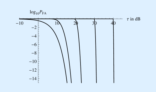
Figure 1: The energy detector log-log plot of $P_{\text{FA}}$ against the normalized threshold $\tau$ for $K=10^{n}$ where $n\in[0,4]$. Larger $K$ have higher $P_{\text{FA}}$ for the same $\tau$, or require larger $\tau$ for the same $P_{\text{FA}}$. Note that the matched filter corresponds to $K=1$, $n=0$, and has the most favorable tradeoff of $\tau$ vs $P_{\text{FA}}$.

A major advantage of the ED is that unlike the MF it does not require knowledge of $\mathbf{h}$, but a substantial penalty is paid in sensitivity for $K>1$. That is one manifestation of a more general principle of signal detection: The more specific the detector’s knowledge of the signal, the better the sensitivity of a detector that makes use of that knowledge. Cyclops [15] prescribed an ED to avoid knowing $\mathbf{h}$, but also prescribed $K\approx 1$ in order to preserve detector sensitivity. Intuitively the penalty for increasing $K=BT$ in the ED arises because more total noise energy is captured in $Z_{\text{E}}$ either because $B$ is large (noise energy equals noise density times bandwidth) or $T$ is large (noise energy equals noise power times integration time). $K\approx 1$ can be accomplished with a carrier-like signal (small $B\approx 1/T$) or a pulse-like signal (small $T\approx 1/B$). In both cases the one DOF specifies the phase and amplitude, and thus this strategy chooses an exact signal waveform $h(t)$ (just as we propose for spread spectrum in Section 4). Small $B$ was preferred in [15] to reduce the transmit power for a given $\mathcal{E}_{h}$.

3.4 Radio-frequency interference

Is there any motivation to increase the signal DOF $K$? First, the information-bearing nature of the PAM signal of (1) is not a motivation, since the only requirement is that (3) be satisfied and this only requires that $K=B\,T\geq 1$. Decreasing $T$ is beneficial because the higher symbol rate implies (all else equal) a higher information rate, and this in turn requires larger $B$ but not larger $K$. The primary penalty for increasing the information rate is higher transmit signal power, since that power is $\mathcal{E}_{h}/T$, and if $h(t)$ is known and a MF is used in the receiver we saw in Section 3.3 that $\mathcal{E}_{h}$ does not depend on $B$, $T$, or $K$ for fixed $P_{\text{FA}}$ and $P_{\text{D}}$. There is, however, one strong motivation for making $K$ large, and that is RFI as we will now see.

Recall from Section 2.3 that the receiver’s immunity to RFI is quantified by the gain $G=FG\times PG$. If, as is likely, the transmitter designer has no specific knowledge of the RFI environment at the receiver, he has no opportunity to manipulate $FG$ through the choice of $T$ and $B$ since the temporal and bandwidth characteristics of the RFI are unknown. However, that designer does have an opportunity to manipulate $PG$ by choosing $K$ to be large. As long as the receiver has knowledge of $h(t)$ and uses that knowledge to construct a MF detector, then the transmitter designer can assume that such a large $K$ has no adverse effect on the detection noise sensitivity. He can therefore focus on choosing $h(t)$ to achieve robust $PG$, meaning the greatest $PG$ that can be consistently achieved without needing to incorporate any specific assumptions about the RFI.

From the transmitter designer perspective, assume the RFI after the benefit of $FG$ is represented by a deterministic (but unknown) vector $\mathbf{r}\in\mathbb{C}^{K}$ in the same basis as the signal vector $\mathbf{h}$, where $\mathbf{r}$ is a unit vector that represents the direction of the RFI in $\mathbb{C}^{K}$ and $\mathcal{E}_{r}$ is the energy of the RFI. If the receiver is presumed to use a MF, then the transmitter designer knows that the component of RFI at the decision threshold is $Z_{\text{M}}=\mathcal{E}_{r}\,{\mathbf{h}}^{\dagger}\mathbf{r}$ , and this term biases the decision in favor of $\mathcal{E}_{h}>0$ and hence increases $P_{\text{FA}}$. In choosing $\mathbf{h}$ the transmitter thus has an interest in making $\left|\,{\mathbf{h}}^{\dagger}\mathbf{r}\,\right|$ as consistently small as possible. The factor by which RFI energy is reduced by the MF is

$$PG=\frac{\left\|\,\mathcal{E}_{r}\,\mathbf{r}\,\right\|^{\,2}}{|\,\mathcal{E}_{r}\,{\mathbf{h}}^{\dagger}\,\mathbf{r}\,|^{\,2}}=\frac{1}{|\,{\mathbf{h}}^{\dagger}\mathbf{r}\,|^{\,2}}\,.$$ (9)

$PG$ depends on the geometric relationship of two unit vectors, $\mathbf{h}$ and $\mathbf{r}$: $PG=1$ when $\mathbf{h}$ is colinear with $\mathbf{r}$, $PG=\infty$ when it is orthogonal, and otherwise $1<PG<\infty$.

How do we achieve consistently large $PG$? Two perspectives arrive at similar conclusions. First, if $\mathbf{h}$ is in some sense spread uniformly throughout $K$ dimensional space, only a fraction $1/K$ of its unit energy will fall in the direction of any $\mathbf{r}$, independent of $\mathbf{r}$. In that case, $PG\approx K$, and there is a clear benefit to making $K$ as large as possible. Second, consider a basis chosen to include $\mathbf{h}$ as the first basis vector. Then two extreme scenarios are the unit energy of $\mathbf{r}$ spread evenly over all basis vectors, in which case only a fraction $1/K$ of the unit energy is co-linear with the one coordinate $\mathbf{h}$, or the unit energy is concentrated in one basis vector, in which case the chance that this vector happens to be the signal direction is only $1/K$ [19]. In either case, $PG\approx K$ in a statistical sense, and we conclude again that large $K$ is advantageous. Nevertheless, $PG\approx 1$ can always occur inadvertently when $\mathbf{h}\approx\mathbf{r}$, even if that outcome is deemed to be unlikely.

Lacking control over or knowledge of $\mathbf{r}$, a communication engineer focuses instead on $\mathbf{h}$, which the transmitter designer chooses. Specifically, the previous argument suggests that he should seek a signal which spreads its energy uniformly throughout the $K$ DOF’s. There is no direct justification for choosing any specific $\mathbf{h}$, either for noise sensitivity or RFI immunity. Thus, the designer can do no better than choose $\mathbf{h}$ as a random vector $\mathbf{H}$ drawn from some appropriate random ensemble. The transmitter will choose $\mathbf{H}$ randomly from this ensemble, and a receiver knowing $\mathbf{H}$ implements a MF using $\mathbf{H}$. The obvious question—how does the receiver know $\mathbf{H}$?— is addressed in Section 4.2. With this approach, the designer can answer two useful questions: First, $PG=1/|{\mathbf{H}}^{\dagger}\mathbf{r}|^{\,2}$ becomes a random variable, and the distribution of $PG$ yields specific information as to how the $PG$ is distributed, and especially how likely it is that $PG$ will be small (the RFI mimics the signal) or large (RFI is highly attenuated by the MF). Second, the designer can ask how the choice of a random ensemble for $\mathbf{H}$ affects the distribution of $PG$, and in particular if there is any choice that renders that distribution independent of $\mathbf{r}$, achieving the goal of robust RFI rejection in a statistical sense.

The IP suggests an immediate answer to the second question because it establishes that the energy of a Gaussian CR $\mathbf{H}$ is the same in any direction and thus the variance $|{\mathbf{H}}^{\dagger}\mathbf{r}|$ does not depend on $\mathbf{r}$. The only problem is that this ensemble does not incorporate the constraint that $\|\mathbf{H}\|\equiv 1$. To address this, let $\mathbf{X}$ be a Gaussian CR random vector, and choose $\mathbf{H}=\mathbf{X}/\|\mathbf{X}\|$. For this choice of $\mathbf{H}$, the distribution function of $PG$ in (9) is ( B)

$$F_{PG}(p)=\text{Pr}\left\{PG\leq p\right\}=\left(1-\frac{1}{p}\right)^{K-1},\;\;p\geq 1\,.$$ (10)

Notably $F_{PG}(p)$ still does not depend on $\mathbf{r}$ and $F_{PG}(p)$ decreases exponentialy with increasing $K$ as illustrated in Figure 2. Any objective for the probability that $PG\leq p$ for any $p>0$ can be met by choosing $K$ sufficiently large. For example, if we require the probability that $PG$ falls below 40 dB to be less than $10^{-10}$, then we must choose $K>230,248$ (e.g. $T=0.1$ sec and $B=2.31$ MHz).

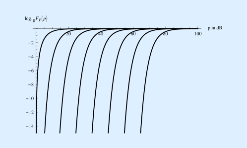
Figure 2: The cumulative distribution function $F_{PG}(p)$ of processing gain $PG$ for a CR signal $\mathbf{H}=\mathbf{X}/\|\mathbf{X}\|$, a Gaussian CR $\mathbf{X}$, and any $\mathbf{r}$. It is plotted on a log-log plot ($10\log_{10}p$ vs $\log_{10}F_{\mathcal{P}}(p)$) for $K=10^{n}$ and $n\in[1,8]$. The distribution moves to the right by approximately 10 dB for every order-of-magnitude increase in $K$.

Consider for example a jammer who deliberately tries to design a worst-case interferer and is aware that $\mathbf{H}$ was chosen as described previously, but is not aware of the specific outcome $\mathbf{H}$. This jammer has no basis for choosing a specific $\mathbf{r}$; that is, no choice is better or worse than any other. There is a duality: Choosing a CR signal $\mathbf{H}$ yields a $PG$ distribution that is independent of $\mathbf{r}$, just as a CR noise $\mathbf{N}$ results in a distribution (the same distribution!) that is independent of $\mathbf{h}$. These two statements are compatible, as any randomly chosen $\mathbf{H}$ in the former is entirely suitable for the latter. For any other way of choosing $\mathbf{H}$, the distribution of $PG$ is dependent on $\mathbf{r}$. That is, some interferers are rejected more than others, and robust immunity is lost.

There are several conclusions. First, there are always values of $\mathbf{r}\approx\mathbf{H}$ for which immunity is poor. In short, beware of impostors. However, the probability of this happening inadvertently can be made arbitrarily small by increasing $K$. Second, $K$ can be chosen freely without penalty in noise sensitivity with a MF; large $K$ is advantageous for RFI immunity and not deleterious to noise immunity. Third, robustness in RFI immunity requires that $\mathcal{E}_{h}$ be spread uniformly over its $K$ DOF’s, and this is achieved if $\mathbf{H}$ is Gaussian CR. Unlike noise immunity, the goal of robust RFI immunity provides specific information about advantageous signal characteristics; namely, the signal should statistically resemble white Gaussian noise.

Choosing the signal from a CR ensemble in conjunction with the MF is an equilibrium strategy in the game theoretic sense. Any deviation from this strategy either degrades the detector sensitivity in noise, or it abandons robustness in RFI rejection, or both. Assuming the receiver designer focuses on the limited information available to the transmitter designer, each will arrive at this same fundamental conclusion based on elementary probability theory. However, turning this principle into a concrete signal design introduces some ambiguity as discussed next.

4 CONCRETE SIGNAL DESIGN

Even acknowledging fundamental principles, obvious questions loom. How do we choose the signal parameters $B$ and $T$? Given that the transmitter cannot communicate a chosen signal $\mathbf{h}$ to the receiver, can we make a credible argument that $\mathbf{h}$ can be guessed by the receiver, or that there are at least a limited number of options that can be searched? In addressing these issues, we draw upon extensive experience in designing terrestrial communication systems.

4.1 Choosing $T$ and $B$

The RFI $PG$ depends only on the time-bandwidth product $K=B\,T$, and thus offers no insight into how a chosen $K$ should be partitioned between $B$ and $T$. This design choice must rely on external considerations such as the transmitter’s stellar scanning dwell time and desired data rate (which influence $T$), impairments in the interstellar medium (which influences $B$), and the receiver’s search strategy. Generally it can be asserted that $T$ is a scarce resource but $B$ is more ample. Another consideration is the RFI $FG$ (Section 2.3), which depends on the anticipated nature of the RFI. For persistent narrowband RFI (like other communication signals) it is more advantageous to increase $B$, but for bursty RFI (like impulsive noise from the electrical grid or motors) it is more advantageous to increase $T$. Finally, many current searches depend entirely on large $FG$ by choosing $K\approx 1$ and thus perform poorly for RFI that mimics the signal’s small time-bandwidth product but relatively well for other types of interferers.

4.2 Pseudorandom signal

In the random signal approach, there is no possibility of communicating $\mathbf{h}$ to the receiver, but the receiver may be able to guess an algorithm used to generate the signal. This suggests using a pseudorandom algorithm (PR) for generating a signal that is representative of the random ensemble. The criterion for ”representative" is meeting standard statistical tests for a sequence that is CR. The significance or reliability of such tests increases with $K$. Although the PR algorithm mimics white Gaussian noise, the receiver searches for a unique signal rather than applying statistical tests to the reception, and thus there is no extra source of confusion with noise when the signal is chosen randomly.

4.3 QPSK signal

To be successful in acquisition, the receiver must guess both the basis functions and the PR algorithm. Of course, in both cases the receiver can search multiple possibilities subject only to computational power (principally budget and technology) limitations and must suffer a penalty in $P_{\text{FA}}$. (There is no possibility of searching over all possibilities, because the $P_{\text{FA}}$ penalty would be too large.) Based on our terrestrial experience, either the sampling theorem (5) or Fourier (6) basis seems a likely choice. When resolving the ambiguity of what PR generator to use, Occam’s razor – look for the simplest solution that meets the requirements – is a good guiding principle [1]. The question then is whether the simplest possible PR generator, one that mimics a sequence of independent coin tosses, can be used. The answer is yes if an independent CR (rather than Gaussian CR) $\mathbf{H}$ can suffice. Fortunately, from Table 3 independent CR vectors obey the energy IP precisely and also approach Gaussian CR in distribution as $K\to\infty$.

The approach used in terrestrial systems is to define a finite constellation from which components of $\mathbf{H}$ are chosen randomly. The smallest complex-valued constellation for the components of $\mathbf{H}$ that can be independent CR and zero mean has four points (these properties are inconsistent with a two- or three-point constellation). This constellation must include the points $(\pm 1\pm i)$, where the real and imaginary components are independent and chosen by a fair coin toss. Suppose a binary PR generator statistically mimics a sequence of $2K$ independent coin tosses $\{c_{l},\,1\leq l\leq 2\,K\}$, where $c_{l}=\pm 1$. Then the vector

$$\mathbf{h}=[c_{1}+i\cdot c_{2},\;c_{3}+i\cdot c_{4},\dots,\;c_{2K-1}+i\cdot c_{2K}]$$

statistically mimics an independent CR random vector $\mathbf{H}$, and it is the simplest choice. This is called a quaternary phase-shift key (QPSK) PR generator, and as expected the distribution of $PG$ for this PR sequence and a Gaussian CR $\mathbf{H}$ are virtually indistinguishable as illustrated in Figure 3.

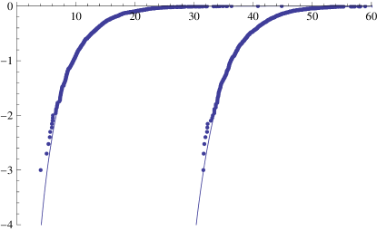
Figure 3: The distribution of RFI $P$ in dB for an interferer consisting of a 64-QAM digital communication signal with random data symbols, one symbol per second, and a 50% excess bandwidth. The two cases shown both assume that $T=10$ seconds, with $B=2$ ($K=20$) and $B=1000$ ($K=10^{4}$). Shown are the results of one million trials of a PR QPSK signal using the RandomTrials[] function of Mathematica. The vertical axis is $\log_{10}$ of the fraction of trials for which $P<p$ and the horizontal axis is $p$ in dB. The solid curve is the theoretical prediction for a Gaussian CR signal.

4.4 The PR open-ended sequence property

Another requirement on the PR algorithm is evident upon examining the basis expansions. The receiver’s computational requirements can be dramatically reduced if a mismatch in DOF $K$ between transmitter and receiver is permitted, and this is permissible as long as the PR sequence $\{c_{k},\;1\leq k<\infty\}$ is open-ended and has an unambiguous initial state. If the bandwidth $B$ remains fixed in (5) and $c_{k}$ is mapped onto coordinates $\mathbf{H}$ with DOF $K$ in the transmitter and $M\neq K$ in the receiver, then detection remains feasible with reduced sensitivity. If $K>M$ then some transmitted energy is lost, if $K<M$ some unnecessary noise is added into the signal level estimate, and maximum sensitivity occurs for $M=K$. The receiver must still search over different values of $B$ (or equivalently different sampling rates), but the value of $T$ can be left open. This required search over $B$ introduces an additional search parameter and increases the computational burden accordingly. Similar logic applies to Fourier basis (6), except that the search is over $T$ and it is $B$ that is left open.

Any discovery algorithm for an information-bearing signal must search over starting time and $f_{c}$. In the discovery of an information-bearing signal (and spread spectrum is no exception) there is one additional dimension to search, which we call a dilation parameter. It can be chosen to be $T$ (equivalent to the frequency sampling or symbol rate $1/T$) or $B$ (equivalent to the time sampling rate $1/B$). The most sensitive detectors will search over both these dilation parameters.

4.5 PR coin-toss generators

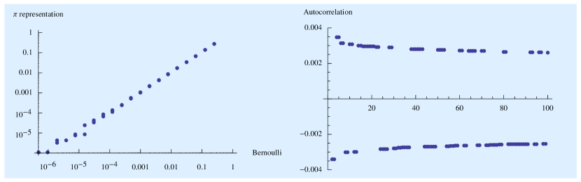
Figure 4: Tests for independent coin-toss statistics for a two million bit binary expansion of $\pi$. On the left, the relative frequency of run lengths of $+1$’s and $-1$’s against the predicted probabilities. The disparities at small relative frequencies is explained by the statistically insignificant number of longer sequences. On the right, the magnitude of the autocorrelation sorted from largest to smallest is plotted with the unity autocorrelation at zero lag omitted. The predicted value of zero is satisfied within a few parts in a thousand.

Because of their explicit coordination, terrestrial systems do not require the open-ended sequence property and hence offer little direct guidance as to choice of a PR algorithm. Nevertheless it is straightforward to find PR algorithms with this property, including ones that rely on nothing more sophisticated than the geometry of the square or the circle. For example, common irrational numbers such as $\pi$, $\sqrt{2}$, and $e$ expanded in base two satisfy the open-ended sequence property and have been observed to satisfy statistical tests for independent and identically distributed coin tosses [42]. If the receiver has to search over $L$ different algorithms, an increase in $\mathcal{E}_{h}$ by $\log L$ is necessary to avoid an increase in overall $P_{\text{FA}}$ [23].

The number $\pi$ seems like a particularly interesting candidate, especially since it has been known and studied centuries and has been confirmed to pass rigorous statistical tests [43]. An example of one such test, the frequency of run lengths, is shown in Figure 4. A run of one +1 followed immediately by a -1 should occur close to one quarter of the time, two +1’s followed by a -1 close to an eighth of the time, etc. Another test of randomness calculates the sample autocorrelation function. Since $E[C_{m}{C}^{\ast}_{n}]=\frac{1}{K}\cdot\delta_{m-n}$ for any white CR vector, at large $K$ the time average autocorrelation should approximate,

$$\sum c_{k}{c}^{\ast}_{k-m}\approx\delta_{m}\,.$$

Equivalently, the Fourier transform of $c_{k}$ should be approximately white (constant magnitude). By the IP, such signals have their energy spread relatively uniformly over both a time basis in $t\in[0,T]$, a frequency basis in $f\in[0,B]$, or indeed any basis. Such a signal appears noise-like and stationary, as illustrated by the $\pi$ representation of Figures 5 and 6.

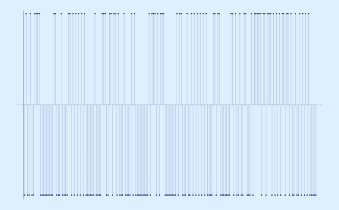
Figure 5: Plot of the real part of a PR signal with $K=100$ based on the first 200 bits of the binary expansion of $\pi$ (typically a much larger $K$ would be used). By construction, the signal energy is spread uniformly over time, and is thus relatively immune to pulse-like RFI.

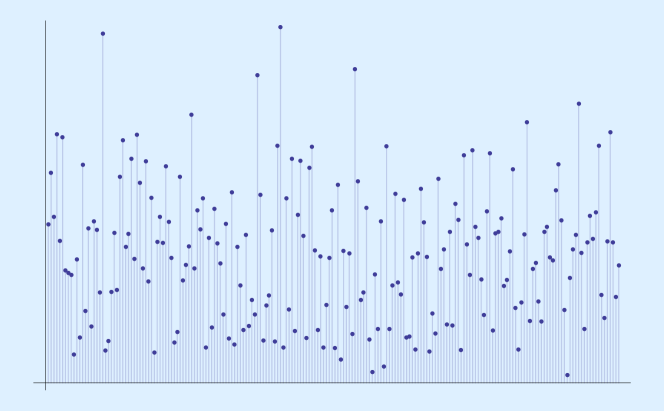
Figure 6: Plot of the magnitude of the discrete Fourier transform of the signal in Figure 5. Reflecting the IP, the signal energy is spread relatively uniformly over frequency, and is thus relatively immune to narrowband RFI. The variation in energy with frequency is consistent with the expected complete randomness.

5 CONCLUSIONS

We have addressed the discovery of an information-bearing signal for interstellar communication in the presence of noise and RFI. Design for maximum detection sensitivity in noise offers no insight into the type of signal to transmit or seek. We have demonstrated that a signal in which each symbol-period pulse $h(t)$ statistically matches a burst of bandlimited white noise is the only choice that achieves robust immunity to RFI (immunity not dependent on the specific in-band RFI waveform) for matched filter detection. This immunity is additive to other forms of RFI mitigation, and works when RFI is overlapping in frequency, time, and space. A signal with this characteristic can be generated by a PR algorithm that we assert can be guessed by the receiver, such as a QPSK constellation in conjunction with the binary expansion of an irrational number like $\pi$. This observation informs both transmitter and receiver designers as to the desirable characteristics of a signal to transmit and to seek.

A consequence of wider signal bandwidth that has not be addressed is its susceptibility to dispersion and multipath distortion introduced in the ISM [22]. While the same can be said of any information-bearing signal as the information rate is increased, spread spectrum increases the severity of this impairment. This is addressed elsewhere [23], where it is shown that there is a quantifiable no-dispersion region of $\{B,\,T,\,f_{c}\}$ for which these effects are insignificant. This observation together with a desire to maximize $K=BT$ suggests transmitting and searching for signals near the boundary of the no-dispersion region, dramatically narrowing the ambiguity in parameters $\{B,\,T,\,f_{c}\}$ for both transmitter and receiver.

Other practical issues are yet to be addressed. What are the consequences of relative motion between transmitter, receiver, and ISM clouds? What about the conversion from continuous-time, and the related granularity in the search space over $\{f_{c},B\}$ or $\{f_{c},T\}$? What are the computational requirements for such a search? How are these parameters related to a stellar scanning strategy?

Appendix A INFORMATION-BEARING SIGNALS

Assuming that the information to be conveyed is digital in nature [30], without loss of generality it can be represented as a sequence of bounded integers $\{I_{k},\ -\infty<k<\infty\}$ where $k$ represents time and $I_{k}\in[1,M]$. The radio electric field is generated by a process of modulation, turning $\{I_{k}\}$ into a continuous-time waveform. In general form, and equivalently at baseband, this waveform is

$$y(t)=\sum_{k=-\infty}^{\infty}h_{I_{k}}(t-kT)\,,$$ (11)

where the $\{h_{l}(t),\,1\leq l\leq M\}$ is a set of $M$ waveforms distinctive in a way that allows the receiver to infer the corresponding $I_{k}$. The raw information rate is $R=(\log_{2}M)/T$ bits per second.

A passband signal at carrier frequency $f_{c}$ can readily convey a complex-valued waveform $y(t)$, which can effectively double or more than double the information rate by allowing a larger $M$. To see this, any real-valued passband signal $x(t)$ with carrier frequency $f_{c}$ can be represented in terms of an equivalent complex-valued baseband $y(t)$ as

$$x(t)=\sqrt{2}\cdot\Re\left\{y(t)\cdot e^{i2\pi f_{c}t}\right\}\,.$$

The $\sqrt{2}$ factor equates the baseband and passband power or energy, and $\Re$ and $\Im$ denote the real and imaginary parts of a complex number. From

$$\sqrt{2}\cdot x(t)\cdot e^{-i2\pi f_{c}t}=y(t)+y^{*}(t)\cdot e^{-i4\pi f_{c}t}\,,$$

and $y(t)$ can recovered from $x(t)$ by lowpass filtering $x(t)\cdot e^{-i2\pi f_{c}t}$.

Prominent special cases are orthogonal signaling, in which the $\{h_{m}(t),\ 1\leq m\leq M\}$ are mutually orthogonal (uncorrelated), and the PAM of (1). FSK and PSK [28] are examples of these two signal classes. Although the choice of $h(t)$ in PAM is emphasized in this paper, the results are readily extended to orthogonal waveforms. The results of this paper thus apply quite generally to any digital communication scheme conforming to (11) (this includes virtually all digital transmission in use terrestrially), but not to analog modulation (which has been prominently applied to some METI experiments [8]).

Appendix B ISOTROPIC PRINCIPLE

The statements in Table 3 will now be verified. A zero-mean complex-valued random vector in $\mathbb{C}^{K}$ can be written as $\mathbf{V}=\mathbf{A}+i\cdot\mathbf{B}$. A full set of second-order statistics include three $K\times K$ covariance matrices: $E[\mathbf{A}{\mathbf{A}}^{\mathsf{T}}]$, $E[\mathbf{A}{\mathbf{B}}^{\mathsf{T}}]$, and $E[\mathbf{B}{\mathbf{B}}^{\mathsf{T}}]$ (${\mathbf{x}}^{\mathsf{T}}$ is the transpose of $\mathbf{x}$). Equivalently we can use two complex-valued matrices (${\mathbf{x}}^{\dagger}$ is the conjugate transpose (Hermitian) of $\mathbf{x}$) as [41]

$$\mathbf{R}_{v}=E\left[\mathbf{V}{\mathbf{V}}^{\dagger}\right]\text{ and }\tilde{\mathbf{R}}_{v}=E\left[\mathbf{V}{\mathbf{V}}^{\mathsf{T}}\right]\,.$$

$\mathbf{R}_{v}$ is the conventional covariance matrix, and $\tilde{\mathbf{R}}_{v}$ is a pseudo-covariance matrix. The equivalence can be verified by writing $\mathbf{R}_{v}$ and $\tilde{\mathbf{R}}_{v}$ in terms of $\mathbf{A}$ and $\mathbf{B}$ and solving for $E[\mathbf{A}{\mathbf{A}}^{\mathsf{T}}]$, $E[\mathbf{A}{\mathbf{B}}^{\mathsf{T}}]$, and $E[\mathbf{B}{\mathbf{B}}^{\mathsf{T}}]$ in terms of $\mathbf{R}_{v}$ and $\tilde{\mathbf{R}}_{v}$. In contrast to the real-valued case, the covariance matrix alone does not completely specify the second-order statistics. Further, it is readily shown that white CR in Table 2 is satisfied if and only if $\mathbf{R}_{v}=\sigma^{\,2}\cdot\mathbf{I}$ and $\tilde{\mathbf{R}}_{v}=\mathbf{0}$.

Let $\mathbf{U}$ be a unitary $K\times K$ matrix (${\mathbf{U}}^{\dagger}\,\mathbf{U}=\mathbf{U}\,{\mathbf{U}}^{\dagger}=\mathbf{I}$) corresponding to a transformation from one orthonormal basis to another. For example $\mathbf{U}$ is the discrete Fourier transform (DFT) when converting from time to Fourier basis. If $\mathbf{V}$ is white CR, then so too is $\mathbf{U}\mathbf{V}$, as verified by

$$E\left[(\mathbf{U}\mathbf{V}){(\mathbf{U}\mathbf{V})}^{\dagger}\right]=\mathbf{U}\,\left(E\left[\mathbf{V}{\mathbf{V}}^{\dagger}\right]\,\right){\mathbf{U}}^{\dagger}=\sigma^{\,2}\cdot\mathbf{U}{\mathbf{U}}^{\dagger}=\sigma^{\,2}\cdot\mathbf{I}$$

$$E\left[(\mathbf{U}\mathbf{V}){(\mathbf{U}\mathbf{V})}^{\mathsf{T}}\right]=E\left[\mathbf{U}\mathbf{V}{\mathbf{V}}^{\mathsf{T}}{\mathbf{U}}^{\mathsf{T}}\right]=\mathbf{U}\,\left(E\left[\mathbf{V}{\mathbf{V}}^{\mathsf{T}}\right]\,\right){\mathbf{U}}^{\mathsf{T}}=\mathbf{0}\,.$$

Since $\mathbf{U}\mathbf{V}$ is Gaussian when $\mathbf{V}$ is Gaussian, a Gaussian CR vector remains Gaussian CR after coordinate transformation.

Consider the distribution of $Z_{\text{M}}$ and $Z_{\text{E}}$ given by (8). By the IP, ${\mathbf{h}}^{\dagger}\,\mathbf{N}_{1}$ is Gaussian with variance $\sigma^{\,2}$ not dependent on $\mathbf{h}$. For any $K\times K$ unitary $\mathbf{U}$, $e^{-i\theta}\cdot\mathbf{U}$ is also unitary and thus (since a unitary transformation is norm-preserving)

$$Z_{\text{E}}=\left\|\sqrt{\mathcal{E}_{h}}\cdot\mathbf{U}\mathbf{h}+\mathbf{N}_{2}\right\|$$

where by the IP since $\mathbf{N}_{1}$ is Gaussian CR then so too is $\mathbf{N}_{2}=e^{-i\theta}\mathbf{U}\mathbf{N}_{1}$. In particular choose any $\mathbf{U}$ such that $\mathbf{U}\mathbf{h}={[1\,0\,0\dots 0]}^{\mathsf{T}}$ ($\mathbf{h}$ is the first column of ${\mathbf{U}}^{\dagger}$, or equivalently the first basis vector). The distribution of $Z_{\text{E}}$ does not depend on $\mathbf{h}$ because the distribution of $\mathbf{N}_{2}$ does not depend on $\mathbf{U}$. For $\mathbf{h}=\mathbf{0}$

$$P_{\text{FA}}=\text{Pr}\left\{Z_{E}>\lambda\right\}=\text{Pr}\left\{\sum_{i=1}^{K}\,\frac{|n_{i}|^{2}}{\sigma^{2}/2}>\frac{2\lambda^{2}}{\sigma^{2}}\right\}\,,$$

where the left side is $\chi^{2}(2K)$, and $P_{\text{FA}}$ can be calculated from the $\chi^{2}$ distribution function as shown in Figure 1. Similarly, $Z_{\text{M}}$ is $\chi^{2}(2)$ and thus has the same distribution as $Z_{\text{E}}$ for $K=1$.

Our interest is in the random variable $PG$ in (9) when $\mathbf{h}$ is a random vector $\mathbf{H}=\mathbf{X}/\|\mathbf{X}\|$, and $\mathbf{X}$ is Gaussian CR. Let $\mathbf{U}$ be any unitary matrix whose first column is $\mathbf{r}$. By the IP, $\mathbf{V}={\mathbf{U}}^{\dagger}\,\mathbf{X}={[V_{1},\,V_{2},\dots,\,V_{K}]}^{\mathsf{T}}$ is also Gaussian CR. Then from the norm preserving property $PG$ is a function of $\mathbf{r}$ but its distribution is not,

$$PG=\frac{\left\|\,\mathbf{X}\,\right\|^{\,2}}{\left|\,{\mathbf{X}}^{\dagger}\,\mathbf{r}\,\right|^{\,2}}=\frac{\left\|\,{\mathbf{U}}^{\dagger}\,\mathbf{X}\,\right\|^{\,2}}{\left|\,{\mathbf{X}}^{\dagger}\,\mathbf{U}{\mathbf{U}}^{\dagger}\,\mathbf{r}\,\right|^{\,2}}=\frac{\left\|\,\mathbf{V}\,\right\|^{\,2}}{\left|\,{\mathbf{V}}^{\dagger}\,{\mathbf{U}}^{\dagger}\,\mathbf{r}\,\right|^{\,2}}=\frac{\left\|\,\mathbf{V}\,\right\|^{\,2}}{\left|V_{1}\,\right|^{\,2}}\,.$$

Letting $W=\sum_{k=2}^{K}\left|V_{k}\right|^{\,2}$ , the distribution function is

$$\text{Pr}\left\{PG\leq p\right\}=\text{Pr}\left\{W\leq(p-1)\cdot\left|V_{1}\right|^{\,2}\right\}=\int_{0}^{\infty}\text{Pr}\left\{w\leq(p-1)\cdot\left|V_{1}\right|^{\,2}\right\}f_{W}(w)\,dw$$

where $W$ is $\chi^{\,2}(2K-2)$ and $\left|V_{1}\right|^{\,2}$ is $\chi^{\,2}(2)$. Evaluating the integral yields (10).

The asymptotic property for an independent CR vector mentioned in Table 3 is significant for characterizing $PG$ when $\mathbf{H}$ is independent CR but not Gaussian (e.g. a QPSK signal drawn from independent coin-tosses). The distribution of ${\mathbf{X}}^{\dagger}\mathbf{r}$ will approach Gaussian as $K\to\infty$ for almost all values of $\mathbf{r}$ since

$${\mathbf{X}}^{\dagger}\,\mathbf{r}=\sum_{k=0}^{K-1}{X}^{\ast}_{k}\,r_{k}$$

is a sum of independent random variables. Although the terms in the summation are not identically distributed, the Lyapunov version of the Central Limit Theorem [44] asserts that $\Re\{{\mathbf{X}}^{\dagger}r\}$ and $\Im\{{\mathbf{X}}^{\dagger}r\}$ approach Gaussian in distribution as $K\to\infty$ if at most a finite number of the $\{r_{k},\;0\leq k<\infty\}$ are zero and the third moments of $\Re\{X_{k},\;0\leq k<\infty\}$ and $\Im\{X_{k},\;0\leq k<\infty\}$ obey certain upper bounds. For the QPSK PR generator of Section 4.3 these third moments are identically zero, so relatively rapid convergence to Gaussian is assured. Could any distributions other than Gaussian result from the sum of independent random variables? Yes, the larger class of stable distributions [45]; however, the only stable distribution with finite variance (and $E|{\mathbf{X}}^{\dagger}r|^{\,2}=\sigma^{\,2}<\infty$) is the Gaussian.

Appendix C NOISE STATISTICS

A noise vector $\mathbf{N}$ that originates as white Gaussian noise on the passband channel is Gaussian CR [30] as long as $f_{c}>B$. $\mathbf{N}$ is Gaussian because the conversion is linear. To demonstrate that $\mathbf{N}$ is also white CR, choose $K$ orthonormal baseband basis functions $\{g_{k}(t),\,1\leq k\leq K\}$ on $t\in[0,T]$, and assume real-valued white Gaussian noise $M(t)$ at passband with autocorrelation $E[M(t)M(s)]=N_{0}\cdot\delta(t-s)$. Then

$$N_{k}=\sqrt{2}\cdot\int_{0}^{T}M(t)e^{-i2\pi f_{c}t}{g}^{\ast}_{k}(t)\,\text{d}t$$

$$E\left[N_{k}N_{m}\right]=2N_{0}\int_{0}^{T}e^{-i4\pi f_{c}t}{g}^{\ast}_{k}(t){g}^{\ast}_{m}(t)\,\text{d}t=0\ \ \ \text{for}\ \ \ f_{c}>B$$ (12)

$$E\left[N_{k}{N}^{\ast}_{m}\right]=2N_{0}\int_{0}^{T}{g}^{\ast}_{k}(t)g_{m}(t)\,\text{d}u=2N_{0}\cdot\delta_{k-m}\,.$$

Note that ${g}^{\ast}_{k}(t){g}^{\ast}_{m}(t)$ falls in frequency band $f\in[0,2B]$, and (12) is a Fourier transform evaluated at frequency $2f_{c}$, which evaluates to zero as long as $2f_{c}>2B$.

REFERENCES

AUTHOR

David G. Messerschmitt is the Roger A. Strauch Professor Emeritus of Electrical Engineering and Computer Sciences (EECS) at the University of California at Berkeley. At Berkeley he has previously served as the Interim Dean of the School of Information and Chair of EECS. He is the co-author of five books, including Digital Communication (Kluwer Academic Publishers, Third Edition, 2004). He served on the NSF Blue Ribbon Panel on Cyberinfrastructure and co-chaired a National Research Council (NRC) study on the future of information technology research. His doctorate in Computer, Information, and Control Engineering is from the University of Michigan, and he is a Fellow of the IEEE, a Member of the National Academy of Engineering, and a recipient of the IEEE Alexander Graham Bell Medal recognizing “exceptional contributions to the advancement of communication sciences and engineering”.

REFERENCES

- [1] D. G. Messerschmitt and I. S. Morrison, “Design of interstellar digital communication links: Some insights from communication engineering,” Acta Astronautica, 2011. doi:10.1016/j.actaastro.2011.10.005.
- [2] G. R. Harp, R. F. Ackermann, S. K. Blair, J. Arbunich, P. R. Backus, and J. Tarter, A new class of SETI beacons that contain information. Communication with Extraterrestrial Intelligence, State University of New York Press, 2011.
- [3] I. S. Morrison, “Detection of antipodal signalling and its application to wideband SETI,” Acta Astronautica, 2011. to appear.
- [4] J. Tarter, “The search for extraterrestrial intelligence (SETI),” Annual Review of Astronomy and Astrophysics, vol. 39, no. 1, pp. 511–548, 2001.
- [5] J. C. Tarter, “SETI 2020: A roadmap for future SETI observing projects,” Proc.SPIE, vol. 4273, pp. 93–103, 2001.
- [6] T. L. Wilson, “The search for extraterrestrial intelligence,” Nature, vol. 409, no. 6823, pp. 1110–1114, 2001.
- [7] A. L. Zaitsev, “METI: Messaging to extraterrestrial intelligence,” Searching for Extraterrestrial Intelligence, pp. 399–428, 2011.
- [8] A. L. Zaitsev, “Sending and searching for interstellar messages,” Acta Astronautica, vol. 63, no. 5-6, pp. 614–617, 2008.
- [9] D. A. Vakoch, Communication with Extraterrestrial Intelligence. State University of New York Press, 2011.
- [10] J. Welch, D. Backer, L. Blitz, D. C. J. Bock, G. C. Bower, C. Cheng, S. Croft, M. Dexter, G. Engargiola, and E. Fields, “The allen telescope array: The first widefield, panchromatic, snapshot radio camera for radio astronomy and seti,” Proceedings of the IEEE, vol. 97, no. 8, pp. 1438–1447, 2009.
- [11] A. L. Zaitsev, “The first musical interstellar radio message,” Journal of Communications Technology and Electronics, vol. 53, no. 9, pp. 1107–1113, 2008.
- [12] D. Goldsmith and T. C. Owen, The search for life in the universe. Univ Science Books, 2001.
- [13] J. Benford, G. Benford, and D. Benford, “Messaging with cost-optimized interstellar beacons,” Astrobiology, vol. 10, no. 5, pp. 475–490, 2010.
- [14] G. Benford, J. Benford, and D. Benford, “Searching for cost-optimized interstellar beacons,” Astrobiology, vol. 10, no. 5, pp. 491–498, 2010.
- [15] “Project Cyclops: A design study of a system for detecting extraterrestrial intelligent life,” tech. rep., Stanford/NASA/Ames Research Center Summer Faculty Program in Engineering Systems Design, 1971.
- [16] H. V. Poor, “Active interference suppression in CDMA overlay systems,” IEEE Journal on Selected Areas in Communications, vol. 19, no. 1, pp. 4–20, 2001.
- [17] L. B. Milstein, “Interference rejection techniques in spread spectrum communications,” Proceedings of the IEEE, vol. 76, no. 6, pp. 657–671, 1988.
- [18] J. D. Laster and J. H. Reed, “Interference rejection in digital wireless communications,” IEEE Signal Processing Magazine, vol. 14, no. 3, pp. 37–62, 1997.
- [19] R. Pickholtz, D. Schilling, and L. Milstein, “Theory of spread-spectrum communications–a tutorial,” IEEE Transactions on Communications, vol. 30, no. 5 Part 2, pp. 855–884, 1982.
- [20] R. Scholtz, “The origins of spread-spectrum communications,” IEEE Transactions on Communications, vol. 30, no. 5, pp. 822–854, 1982.
- [21] B. J. Rickett, “Radio propagation through the turbulent interstellar plasma,” Annual Review of Astronomy and Astrophysics, vol. 28, no. 1, pp. 561–605, 1990.
- [22] S. K. Blair, D. G. Messerschmitt, J. Tarter, and G. R. Harp, The Effects of the Ionized Interstellar Medium on Broadband Signals of Extraterrestrial Origin. Communication with Extraterrestrial Intelligence, State University of New York Press, 2011.
- [23] D. G. Messerschmitt, “Interstellar spread-spectrum communication: Receiver design for plasma dispersion,” draft awaiting publication available at www.eecs.berkeley.edu/~messer.
- [24] H. W. Jones, “Optimum signal modulation for interstellar communication,” in Astronomical Society of the Pacific Conference Series (G. S. Shostak, ed.), vol. 74, p. 369, 1995. Accessed at http://www.aspbooks.org/a/volumes on 18 Feb. 2010.
- [25] P. F. Clancy, “Some advantages of wide over narrow band signals in the search for extraterrestrial intelligence/seti,” Journal of the British Interplanetary Society, vol. 33, pp. 391–395, 1980.
- [26] N. Cohen and D. Charlton, “Polychromatic SETI,” Astronomical Society of the Pacific Conference Series, 1995.
- [27] G. S. Shostak, “SETI at wider bandwidths?,” Progress in the Search for Extraterrestrial Life, ed.G.Seth Shostak, ASP Conference Series, vol. 74, 1995.
- [28] P. A. Fridman, “SETI: The transmission rate of radio communication and the signal’s detection,” Acta Astonautica, vol. 69, p. 777, 2011.
- [29] J. Cordes and W. Sullivan, “Astrophysical coding: New approach to SETI signals. I. signal design and wave propagation,” 1995. Accessed at http://www.aspbooks.org/a/volumes on 18 Feb. 2010.
- [30] J. R. Barry, E. A. Lee, and D. G. Messerschmitt, Digital communication. Boston: Kluwer Academic Publishers, 3rd ed., 2004.
- [31] A. R. Thompson, T. E. Gergely, and P. A. V. Bout, “Interference and radioastronomy,” Physics Today, vol. 44, p. 41, 1991.
- [32] R. Ekers and J. Bell, “Radio frequency interference,” in The Universe at Low Radio Frequencies, vol. 199, p. 498, 2002.
- [33] P. Fridman and W. Baan, “RFI mitigation methods in radio astronomy,” Astronomy and Astrophysics, vol. 378, no. 1, pp. 327–344, 2001.
- [34] C. Sagan, “Extraterrestrial intelligence: An international petition,” Science (New York, N.Y.), vol. 218, p. 426, Oct 29 1982. JID: 0404511; ppublish.
- [35] J. Heidmann, “Recent progress on the lunar farside crater saha proposal,” Acta Astronautica, vol. 46, no. 10-12, pp. 661–665, 2000.
- [36] S. Bretteil and R. Weber, “Comparison of two cyclostationary detectors for radio frequency interference mitigation in radio astronomy,” Radio Science, vol. 40, no. 5, p. RS5S15, 2005.
- [37] A. Leshem, A. J. van der Veen, and A. J. Boonstra, “Multichannel interference mitigation techniques in radio astronomy,” The Astrophysical Journal Supplement Series, vol. 131, p. 355, 2000.
- [38] D. R. Lorimer and M. Kramer, Handbook of pulsar astronomy. Cambridge Univ Pr, 2005.
- [39] J. V. Korff, P. Demorest, E. Heien, E. Korpela, D. Werthimer, J. Cobb, M. Lebofsky, D. Anderson, B. Bankay, and A. Siemion, “Astropulse: A search for microsecond transient radio signals using distributed computing. I. methodology,” submitted to Astrophys.J, 2011.
- [40] H. Pollak and D. Slepian, “Prolate spheroidal wave functions, fourier analysis and uncertainty.,” Bell Syst.Tech.Journal, vol. 40, p. 43, 1961.
- [41] D. Tse and P. Viswanath, Fundamentals of wireless communication. Cambridge Univ Pr, 2005.
- [42] B. R. Johnson and D. J. Leeming, “A study of the digits of , and certain other irrational numbers,” Sankhya: The Indian Journal of Statistics, pp. 183–189, 1990.
- [43] T. Jaditz, “Are the digits of an independent and identically distributed sequence?,” American Statistician, pp. 12–16, 2000.
- [44] R. B. Ash, Measure, integration, and functional analysis. Academic Press, second ed., 1999.
- [45] J. P. Nolan, Stable Distributions - Models for Heavy Tailed Data. Boston: Birkhauser, 2010. Accessed at http://academic2.american.edu/ jpnolan/stable/chap1.pdf on 19 Feb. 2010.