Ab-initio elastic tensor of cubic Ti_0.5Al_0.5N alloy: the dependence of the elastic constants on the size and shape of the supercell model

Abstract

In this study we discuss the performance of approximate SQS supercell models in describing the cubic elastic properties of B1 (rocksalt) Ti_0.5Al_0.5N alloy by using a symmetry based projection technique. We show on the example of Ti_0.5Al_0.5N alloy, that this projection technique can be used to align the differently shaped and sized SQS structures for a comparison in modeling elasticity. Moreover, we focus to accurately determine the cubic elastic constants and Zener’s type elastic anisotropy of Ti_0.5Al_0.5N. Our best supercell model, that captures accurately both the randomness and cubic elastic symmetry, results in $C_{11}=447$ GPa, $C_{12}=158$ GPa and $C_{44}=203$ GPa with 3% of error and $A=1.40$ for Zener’s elastic anisotropy with 6% of error. In addition, we establish the general importance of selecting proper approximate SQS supercells with symmetry arguments to reliably model elasticity of alloys. In general, we suggest the calculation of nine elastic tensor elements - $C_{11}$, $C_{22}$, $C_{33}$, $C_{12}$, $C_{13}$, $C_{23}$, $C_{44}$, $C_{55}$ and $C_{66}$, to evaluate and analyze the performance of SQS supercells in predicting elasticity of cubic alloys via projecting out the closest cubic approximate of the elastic tensor. The here described methodology is general enough to be applied in discussing elasticity of substitutional alloys with any symmetry and at arbitrary composition.

I Introduction

TiAlN coatings with their good oxidation resistance and excellent mechanical properties have attracted high technological and academic interest HÖRLING et al. . Several studies have been devoted to discuss these alloys from different aspects to extend our understanding in maximizing their functionality and operational efficiency. The thermodynamics, phase stability and spinodal decomposition in TiAlN have been analyzed Mayrhofer et al. (2006); Alling et al. (2007), also on the influence of nitrogen off-stoichiometry Alling et al. (2008) and pressure Alling et al. (2009). Furthermore, the theoretical prediction of the mixing enthalpy when alloying TiAlN with Cr has resulted in a general design route to improve the thermal stability of hard coatings Lind et al. (2003). Recently, the importance of the significant elastic anisotropy in TiAlN on the isostructural spinodal decomposition has been disccussed Tasnádi et al. (2010); Abrikosov et al. (2010). Though, the available theoretical tools with the help of modern supercomputers allows us to tackle such complex physical phenomena in alloys Ruban and Abrikosov (2008), the prediction of anisotropic tensorial materials properties of substitutional alloys from first principles remains a challenging and highly requested task in computational materials science Liu et al. (2005); van de Walle (2008). For example, in dynamical simulations suitably designed simulation cells can greatly reduce the computational costs of predicting the temperature dependence of the elastic and piezoelectric tensors of alloys. The importance of the elastic and piezoelectric tensors of materials can be underlined not only by its fundamental role in materials science but also their distinguished usage in (micro)mechanical modeling, engineering or designing of machine elements, sensors, telecommunication devices, aircrafts, etc..

Although the ordinary scalar cluster expansion Asta et al. (1991) offers an exact treatment of the thermodynamics of alloys and its tensorial generalization van de Walle (2008) gives the most elegant description of anisotropic tensorial materials quantities of alloys, the computationally less demanding and less complex special quasirandom structure (SQS) approach Zunger et al. (1990) is more favorized due to its simplicity and success. For example the giant piezoelectric response of ScAlN alloys Tasnádi et al. (2010); Wingqvist et al. (2010) or the mechanical properties of TiAlN Tasnádi et al. (2010) have been successfully described within this approach. Using different superstructures, Mayrhofer et al. have discussed the impact of the microscopic configurational freedom on the structural, elastic properties and phase stability in TiAlN Mayrhofer et al. (2006). In B-doped wurtzite AlN significant configurational dependence of the piezoelectric constant has been predicted Tasnádi et al. (2009) with presuming wurtzite symmetry, similarly to the discussion of electronic properties and nonlinear macroscopic polarization in III-V nitride alloys Mäder and Zunger (1995); Bernardini et al. (2001).

In fact, in these studies the success of the SQS approach in describing the energetics of alloys is presumed for predicting tensorial materials properties when using different approximate SQS supercells or even ordered structures. These works were either only predictive on the materials constants or the confirmation of the applied approximate structural model was based on the experimental agreement of the results. Moreover, most of the previous theoretical works on predicting elasticity and piezoelectricity of alloys presumed the experimentally observed symmetry for the modeling SQS supercells, though the substitutional disorder of the atoms in general breaks the local point symmetry of the supercell, and focused only on the corresponding principal symmetry non-equivalent tensor elements. While the symmetry arguments based tensorial version of the cluster expansion van de Walle (2008) gives an exact approach to completely include the local point symmetry of the materials, improperly chosen SQS supercells may result in large discrepancy between theory and experiments or in erroneous theoretical findings.

The SQS approach, in principle, is not aimed to generate structures with the inclusion of local point symmetry and thus to provide the proper, full description of tensorial properties of alloys. In fact, different SQS supercells break the symmetry somewhat differently and thus the comparison of the differently shaped and sized SQS supercells in terms of modeling the elasticity of cubic Ti_0.5Al_0.5N is a rather complex issue. Hence, detailed systematic studies on the application of SQS supercells in predicting elastic constants of alloys are required to establish their performance and to determine their applicability limits. For example, J. von Pezold et al. von Pezold et al. (2010) have recently evaluated the performance of symmetricaly shaped - ($A\times A\times A$), supercells for the description of elasticity in substitutional AlTi alloys and obtained convergence and error bars for the cubic-averaged principle cubic elastic constants within the supercell configuration space. However, a general concept of comparing and measuring different sized and shaped SQS supercells in describing tensorial materials properties is still lacking.

In this study, we present a general projection approach to establish a way of comparing the ab-initio calculated elastic constants of B1 Ti_0.5Al_0.5N obtained with applying different sized and shaped SQS supercells. We accurately predict and extensively discuss the calculation of the principal cubic elastic constants of B1 Ti_0.5Al_0.5N within the SQS approach. In general, we establish the importance of selecting proper SQS supercells with symmetry arguments to reliably model elasticity of alloys. Namely, we show that supercells even with good short range order (SRO) parameters may result in large non-cubic elastic constants and, on the contrary, supercells with bad SRO parameters might approximate cubic elastic symmetry fairly accurately. We give the convergence of elasticity with respect to different SQS supercells for B1 Ti_0.5Al_0.5N via the symmetry projected cubic elastic constants. Moreover, we suggest the calculation of 9 elastic tensor elements - $C_{11}$, $C_{22}$, $C_{33}$, $C_{12}$, $C_{13}$, $C_{23}$, $C_{44}$, $C_{55}$ and $C_{66}$, instead of 21, to evaluate and analyze the performance of SQS supercells in predicting elasticity of cubic alloys.

II Method

In this section we provide a description of the techniques we applied to calculate and analyze the approximate elastic constants of cubic B1 Ti_0.5Al_0.5N alloy. First we explain the applied special quasirandom structure (SQS) approach of modeling alloys and discuss the difficulties of describing the proper symmetric tensorial materials constants within the model. After that, we summarize the computational details of obtaining the energetics and extracting the elastic tensors of the approximate SQS supercells. Finally, we present a general projection method that provides a technique to compare and analyze the calculated approximate elastic tensors and what establishes a principle to discuss the supercell models in terms of modeling elasticity with the inclusion of local point symmetry. The here described methodology is general enough to be applied for substitutional alloys with any symmetry and arbitrary composition.

II.1 Special quasirandom structure approach and its symmetry

The special quasirandom structure (SQS) approach Zunger et al. (1990) greatly reduces the computational difficulties of modeling thermodynamics, mechanical and electronic materials properties of random alloys. The approach models the substitutional disordered alloys with ordered superstructures. The basic structural element of the SQS model is a supercell, what is aimed to capture the structural short range order (SRO) in alloys while its periodic repetition introduces spatial long range order (LRO) Mäder and Zunger (1995). The degree of SRO is usually measured by the Warren-Cowley parameter Cowley (1950), which for a pseudobinary A_1-xB_xN alloy is defined as $\alpha_{j}=1-P_{B}(R)/x_{B}$, where $P_{B}(R)$ is the probability of finding a $B$ atom at a distance $R$ from an $A$ atom and $x_{B}$ stands for the concentration of $B$. A perfectly random alloy is characterized by vanishing SRO, while $\alpha>0$ and $\alpha<0$ define clustering and ordering, respectively. In terms of modeling disorder, approximate SQS supercells with with small or vanishing SROs up to a certain neighboring order can be compared if and only if the interaction parameters are also known. In this work the atomic configurations in the supercells were obtained by including the Warren-Cowley SRO parameters of the first seven nearest-neighboring shells. Namely, the disorder has been considered up to the seventh neighboring shell on the metal sublattice. Accordingly, the SRO parameters were calculated only on the Ti-sublattice. In order to achieve the closest possible model of the perfectly random alloy in the chosen sized and shaped supercell approximation $(A\times B\times C)$, a Metropolis-type simulated annealing algorithm Metropolis et al. (1953) has been applied with a cost-function built from the properly weighted nearest-neighbor SRO parameters.

The SQS supercell approach in general breaks the local point symmetry at different stages. The substitutional disorder changes the microscopic local environments which results also in some distorsions on the lattice parameters. Namely, after full relaxation the supercells will have a general triclinic shape. Moreover, the SQS approach in modeling the substitutional disorder of alloys allows one to apply arbitrary supercell shape and size - $(A\times B\times C)$ in terms of lattice vectors. This arbitrariness though increases the variational freedom to obtain closely vanishing SRO parameters with relative small supercell size at any alloy composition, it also spoils the symmetry of the model. Thus, the elasticity of the B1 Ti_0.5Al_0.5N alloy is modeled with fully relaxed SQS supercells an it is described by 21 elastic constants, instead of the three principal cubic constants, $C_{11}$, $C_{12}$ and $C_{44}$. Namely, in the SQS approach the elastic tensor of the model belongs to a symmetry class that is lower than the one that the alloy shows experimentally. Furthermore, different SQS supercells break the symmetry somewhat differently, which means that the comparison of the results can only be done after certain alignment. In this study we show that a projection technique can provide such an alignment in the example of the B1 Ti_0.5Al_0.5N alloy.

II.2 Calculational technique to obtain the elastic tensors

To obtain total energies and extract the elastic constants of the supercells introduced above, Density Functional Theory (DFT) calculations have been performed with using the plane-wave ultrasoft pseudo-potential Vanderbilt (1990) based Quantum Espresso program package Giannozzi et al. (2009). The exchange correlation energy was approximated by the Perdew-Burke-Ernzerhof generalized gradient functional (PBE-GGA) Perdew et al. (1996). The plane-wave cutoff energy together with the Monkhorst-Pack sampling Monkhorst and Pack (1976) of the Brillouine zone were tested and sufficient convergence was achieved. The pseudopotentials were downloaded from the library linked to Quantum Espresso and tested by calculating the elasticity of bulk B1 AlN and TiN in agreement with literature values Chen et al. (2003); Mayrhofer et al. (2006). In obtaining the ground state structure of the modeling supercells, both the lattice parameters and the internal atomic coordinates were relaxed by using the extended molecular dynamics method with variable cell shape introduced by Wentzcovitch Wentzcovitch et al. (1993). Accordingly, during the relaxation the supercells geometries have been changed from the initial cubic-like lattice structure and converged to a slightly distorted triclinic shape with vanishing stress tensor. Thus, we avoid any residual structural stresses, which is essential in performing an accurate comparative analysis of the calculated elastic tensors. In this dynamics, a value of 0.02 KBar was taken as convergence threshold for the pressure. The elastic constants were calculated via the second order Taylor expansion coefficients of the total energy

$$C_{ij}=\frac{1}{V_{0}}\frac{\partial^{2}E(\epsilon_{1},\ldots,\epsilon_{6}))}{\partial\epsilon_{i}\partial\epsilon_{j}}\Big{|}_{0}$$ (1)

where Voigt’s notation is used to describe the strain $\epsilon$ and elastic $C_{ij}$ tensor Vitos (2010); Nye (1985). To obtain the entire elastic tensor, namely the 21 elastic constants of each supercell, 21 different distorsions have been applied without volume conservation. The elastic constants were calculated by standard finite difference technique from total energy data obtained from $\pm$ 1% and $\pm$2% distorsions.

II.3 Projection of the elastic tensor to the closest elastic tensor of higher symmetry

In this section we describe the projection technique introduced by Moakher et al. Moakher and Norris (2006) to obtain the closest elastic tensor with higher symmetry class for any given elastic tensor with arbitrary symmetry. This projection technique allows us to extract the largest cubic part of the calculated elastic tensors. It introduces a tool to compare the obtained approximate elastic tensors and measure the appropriateness of the SQS supercells in modeling the elasticity of B1 Ti_0.5Al_0.5N.

The symmetric elastic tensor has 21 inequivalent elements for the most general triclinic system. A system with higher point symmetry requires less parameters in describing its elastic behavior. For example, with cubic symmetry the material has only 3 principal elastic constants, $C_{11},C_{12}$ and $C_{44}$, while the hexagonal point symmetry results in 5 elastic constants, $C_{11},C_{12},C_{13},C_{33}$ and $C_{44}$. Nevertheless, any elastic tensor can be expressed as a vector in a 21 dimensional vector space, with the following components

$$E=(C_{11},C_{22},C_{33},\sqrt{2}C_{23},\sqrt{2}C_{13},\sqrt{2}C_{12},2C_{44},2C_{55},$$

$$2C_{66},2C_{14},2C_{25},2C_{36},2C_{34},2C_{15},2C_{26},2C_{24},$$

$$2C_{35},2C_{16},2\sqrt{2}C_{56},2\sqrt{2}C_{46},2\sqrt{2}C_{45}),$$ (2)

where the $\sqrt{2}$’s ensure the invariance of the norm on the representation, whether it is vector or matrix. For the basis vectors see Ref.Browaeys and Chevrot (2004). The following projectors $P_{\text{sym}}$ generate the closest elastic tensor with higher symmetry via

$$E^{\text{sym}}=P^{\text{sym}}E,$$ (3)

where $E_{\text{sym}}$ has higher point symmetry. The term closest here is used in the sense, that the Euclidean distance $||E-E^{\text{sym}}||$ is minimum.

To obtain the closest cubic approximate in our study of B1 Ti_0.5Al_0.5N, we applied the projector given as a 21$\times$21 matrix,

$$P^{\text{cub}}=\begin{pmatrix}p_{\text{cub}}&0_{9\times 12}\\ 0_{12\times 9}&0_{12\times 12}\end{pmatrix},$$

$$p^{\text{cub}}=\begin{pmatrix}1/3&1/3&1/3&0&0&0&0&0&0\\ 1/3&1/3&1/3&0&0&0&0&0&0\\ 1/3&1/3&1/3&0&0&0&0&0&0\\ 0&0&0&1/3&1/3&1/3&0&0&0\\ 0&0&0&1/3&1/3&1/3&0&0&0\\ 0&0&0&1/3&1/3&1/3&0&0&0\\ 0&0&0&0&0&0&1/3&1/3&1/3\\ 0&0&0&0&0&0&1/3&1/3&1/3\\ 0&0&0&0&0&0&1/3&1/3&1/3\\ \end{pmatrix}.$$

(4)

Accordingly, the projected cubic elastic constants can be achieved via the following simple averaging,

$$\bar{C}_{11} = \frac{C_{11}+C_{22}+C_{33}}{3}$$

$$\bar{C}_{12} = \frac{C_{12}+C_{13}+C_{23}}{3}$$

$$\bar{C}_{44} = \frac{C_{44}+C_{55}+C_{66}}{3}.$$ (5)

We can call them cubic-averaged elastic constants, since the equation is equivalent with averaging over the three orthogonal directions, [100], [010] and [001]. We note here that this averaging was used by von Pezold et al. in searching for optimized supercell in AlTi alloys. Thus, to obtain the closest cubic projection of an elastic tensor with arbitrary symmetry one needs to derive 9 different distorsion and calculate 9 independent tensor elements, like $C_{11},C_{22},C_{33},C_{23},C_{13},C_{12},C_{44},C_{55}$ and $C_{66}$. In case of cubic symmetry Eq.(5) results in the well-known cubic identities of the elastic constants, see Eq.(9). For modeling elasticity in hexagonal alloys, one needs the closest hexagonal approximation that can be obtained via the projector

$$P^{\text{hex}}=\begin{pmatrix}p_{\text{hex}}&0_{9\times 12}\\ 0_{12\times 9}&0_{12\times 12}\end{pmatrix},\quad p^{\text{hex}}=\begin{pmatrix}3/8&3/8&0&0&0&1/(4\sqrt{2})&0&0&1/4\\ 3/8&3/8&0&0&0&1/(4\sqrt{2})&0&0&1/4\\ 0&0&1&0&0&0&0&0&0\\ 0&0&0&1/2&1/2&0&0&0&0\\ 0&0&0&1/2&1/2&0&0&0&0\\ 1/(4\sqrt{2})&1/(4\sqrt{2})&0&0&0&3/4&0&0&-1/(2\sqrt{2})\\ 0&0&0&0&0&0&\frac{1}{3}&\frac{1}{3}&0\\ 0&0&0&0&0&0&\frac{1}{3}&\frac{1}{3}&0\\ 1/4&1/4&0&0&0&-1/(2\sqrt{2})&0&0&1/2\end{pmatrix},$$

that acts in the same 9 dimensional subspace and results in the following expressions for the projected hexagonal elastic constants,

$$\bar{C}_{11}=3(C_{11}+C_{22})/8+C_{12}/4+C_{66}/2,\quad\bar{C}_{12}=(C_{11}+C_{22})/2+3C_{12}/4-C_{66}/2,$$

$$\bar{C}_{13}=(C_{13}+C_{23})/2,\quad\bar{C}_{33}=C_{33},\quad\bar{C}_{44}=(C_{44}+C_{55})/2.$$ (7)

A detailed derivation of the projectors for the all symmetry classes, monoclinic, orthorombic, tetragonal, trigonal, hexagonal, cubic and isotropic can be found in Ref. Browaeys and Chevrot (2004); Moakher and Norris (2006). It is worth to mention that not all projectors can be defined in the above used 9 dimensional subspace. Furthermore, the application of this projection technique allows one to spilt the elastic tensor into a direct sum of tensors with different symmetry. Such decomposition is possible, for example, on the following routes,

$$E = E_{\text{cubic}}+E_{\text{tetragonal}}+E_{\text{orthorombic}}$$

$$+E_{\text{monoclinic}}+E_{\text{triclinic}}$$

$$E = E_{\text{hexagonal}}+E_{\text{tetragonal}}+E_{\text{orthorombic}}$$ (8)

$$+E_{\text{monoclinic}}+E_{\text{triclinic}}.$$

Thus, with calculating the norm of the components one gets information about the different contributions and can analyze elastic anisotropy in general Browaeys and Chevrot (2004).

III Results and discussion

In this section we present a comparative analysis of the calculated approximate elastic tensors obtained for the cubic (B1) TiA_0.5l_0.5N alloy within the special quasirandom structure approach. To get different levels of the approximation of the elasticity in cubic Ti_0.5Al_0.5N, several approximate SQS supercell models have been generated with different shape and size, such as $(2\times 2\times 2)$, $(2\times 3\times 2)$, $(4\times 3\times 2)$, $(4\times 3\times 4)$, $(4\times 4\times 3)$ and $(4\times 4\times 4)$. Here SQS supercell sizes are measured in terms of the fcc unit vectors. To have a more complete comparison of the calculated elastic tensors, we present results obtained with the ordered L1₀ structure and three other structures, denoted here by C1-$(2\times 2\times 2)$, C3-$(2\times 2\times 2)$ and B1-$(2\times 2\times 2)$. These three structures are not based on the fcc unit cell but on the fcc Bravais cell. The C1-$(2\times 2\times 2)$ and C3-$(2\times 2\times 2)$ was created by Mayrhofer et al. Mayrhofer et al. (2006) with considering the number of bonds between the host and doping atoms. The C3-$(2\times 2\times 2)$ structure was designed with preserving the cubic symmetry. The B1-$(2\times 2\times 2)$ structure was obtained by von Pezold with using a Monte-Carlo scheme and averaging over the three orthogonal main crystallographic directions. The SRO parameters of all superstructures are summarized in Table 1.

Table 1: The Warren-Cowley pair short range order parameters (SROs) up to the 7th neighboring shell for each SQS supercell considered in this work.

str.$\setminus$shell	number of atoms	$1$	$2$	$3$	$4$	$5$	$6$	$7$
L10	$8$	$-1.0$	$-1.0$	$-1.0$	$-1.0$	$-1.0$	$-1.0$	$-1.0$
(2$\times$2$\times$2)	$16$	$-0.16$	$0.0$	$-0.16$	$1.0$	$-0.16$	$0.0$	$-0.16$
(2$\times$3$\times$2)	$24$	$-0.11$	$0.0$	$-0.08$	$0.33$	$-0.06$	$-0.08$	$0.03$
(4$\times$3$\times$2)	$48$	$0.0$	$0.0$	$0.0$	$0.0$	$-0.06$	$0.0$	$0.0$
(4$\times$3$\times$2)∗	$48$	$-0.14$	$0.28$	$-0.10$	$0.14$	$0.0$	$-0.17$	$-0.01$
C1-(2$\times$2$\times$2)	$64$	$-0.33$	$1.0$	$-0.33$	$1.0$	$-0.33$	$1.0$	$-0.33$
C3-(2$\times$2$\times$2)	$64$	$0.0$	$-1.0$	$0.0$	$-1.0$	$0.0$	$-1.0$	$0.0$
B1-$(2\times 2\times 2)$	$64$	$0.0$	$0.0$	$0.0$	$-0.33$	$0.0$	$0.0$	$0.0$
(4$\times$3$\times$4)	$96$	$0.0$	$0.0$	$0.0$	$0.0$	$0.0$	$0.0$	$0.0$
(4$\times$4$\times$3)	$96$	$0.0$	$0.0$	$-0.01$	$-0.01$	$-0.01$	$0.0$	$0.0$
(4$\times$4$\times$4)	$128$	$0.0$	$0.0$	$0.0$	$0.0$	$0.0$	$0.0$	$0.0$

In the case of the $(2\times 2\times 2)$, $(2\times 3\times 2)$ and $(4\times 4\times 4)$ supercells, those atomic configrations have been chosen that resulted closest to randomness in our approximation, i.e. almost vanishing SRO parameters up to the seventh neighbor shell. The larger SROs in case of the $(2\times 2\times 2)$ supercell are the consequence of the low configurational freedom in the supercell and indicate less perfection in the randomness. In the case of the $(4\times 3\times 2)$ supercell size two different atomic configurations have been considered with very different SRO parameters. The $\ast$ marks the SQS structure that is less random. The calculated SROs of the C1-$(2\times 2\times 2)$ and C3-$(2\times 2\times 2)$ structures show alternating systematics that is related to the used construction strategy. The SRO parameters deviate considerably from zero in these two cases. For example, the cubic symmetric C3-$(2\times 2\times 2)$ shows perfect ordering in every second neighboring shell. In comparing the SRO values in Table 1, the $(4\times 4\times 4)$ supercell gives unambiguously the closest model of a totally random(pseudo-)binary alloy in our SQS approximation.

The structural optimization of these supercells resulted in slight structural distorsions, what are summarized in Table 2.

Table 2: The optimized structural parameters of Ti_0.5Al_0.5N obtained with different supercells from Table 1.

str.	$a(\text{\AA})$	$b(\text{\AA})$	$c(\text{\AA})$	$\measuredangle(b,c)$	$\measuredangle(a,c)$	$\measuredangle(a,b)$
L10	4.17	4.17	4.24	90.00	90.00	90.00
(2$\times$2$\times$2)	4.18	4.18	4.22	59.72	59.72	59.73
(2$\times$3$\times$2)	4.20	4.19	4.17	60.17	60.12	59.65
(4$\times$3$\times$2)	4.18	4.18	4.20	59.67	59.79	59.99
(4$\times$3$\times$2)∗	4.19	4.19	4.17	60.14	60.17	59.66
C1-(2$\times$2$\times$2)	4.25	4.16	4.16	90.00	90.00	90.00
C3-(2$\times$2$\times$2)	4.18	4.18	4.18	90.00	90.00	90.00
B1-(2$\times$2$\times$2)	4.18	4.18	4.18	89.78	89.78	90.00
(4$\times$3$\times$4)	4.20	4.15	4.18	60.26	59.91	60.38
(4$\times$4$\times$3)	4.19	4.18	4.16	60.15	60.13	59.94
(4$\times$4$\times$4)	4.18	4.18	4.19	59.93	60.08	60.00

Table 2 gives the size resolved lattice parameters of B1 Ti_0.5A_0.5lN within the different SQS supercell models. The lattice parameters, especially the length of the cell edges, show some noticeable deviation from the cubic structure, but only for the L1₀, $(2\times 2\times 2)$ and C1-$(2\times 2\times 2)$ supercells. What correlates with the systematic alternation of the large SRO parameters of these cells. This suggests that the observed structural deviation is related to the low degree of freedom of internal atomic arrangement. In the other supercells with higher substitutional atomic disorder/randomness the cubic imperfection is nearly negligible.

For each of these structures the full elastic tensor has been calculated. The elastic constants were obtained independently, as 21 different distorsions were applied. The obtained elastic tensors are summarized for all the structures in Appendix A. All the obtained tensors exhibit deviations from a strict cubic symmetry, in which the principal non-vanishing elements should show the following relationships,

$$\bar{C}_{11}=C_{11}=C_{22}=C_{33},\quad\bar{C}_{12}=C_{12}=C_{13}=C_{23},$$

$$\bar{C}_{44}=C_{44}=C_{55}=C_{66}.$$ (9)

Appendix BB also lists the elastic tensors of bulk B1 TiN and AlN obtained with the supercell size $(4\times 4\times 3)$, where one finds the cubic symmetry of elasticit constants with numerical error. The values show good agreement with the literature data Chen et al. (2003); Mayrhofer et al. (2006) obtained with different techniques. As the C3-$(2\times 2\times 2)$ supercell preserves the cubic symmetry, its elastic tensor shows the cubic relationships in Eq.(9). The non-vanishing other elements define the numerical accuracy, i.e. the average error $(6/463+6/182+6/156)/3$ should be around 3%. Since one gets the same 3% numerical error in the case of bulk B1 TiN and a negligible one for B1 AlN, we can assume that 3% is numerical error threshold for all of our results through the following analysis. One can read from the data in Appendix B that some of the SQS supercells result in large non-cubic elements and large deviations between the principal cubic elastic constants, which means a breakdown of the cubic symmetry relations in Eq.(9). Nevertheless, by the previously introduced projection we can extract the closest cubic elastic tensors and calculate the distance variations $||E-E^{\text{cub.}}||/||E||$. These deviations are shown in Fig.1. The required 9 elastic constants are summarized in Table 3, while the obtained projected cubic elastic constants are listed in Table 4.

Figure 1: (Color online) Calculated euclidian norm deviations $||E-E^{\text{cub}}||/||E||$ obtained in the 21 dimensional space, see Eq.(2).

Table 3: The calculated GGA elastic tensor elements of Ti_0.5Al_0.5N from Appendix B, whichs are involved in the cubic projection, see Eqs.(4) and (5).

str.$\setminus$const.	$C_{11}$	$C_{22}$	$C_{33}$	$C_{12}$	$C_{13}$	$C_{23}$	$C_{44}$	$C_{55}$	$C_{66}$
TiN	617	618	618	123	123	123	178	178	178
AlN	402	402	402	157	157	157	300	300	300
L10	409	409	332	183	197	197	100	100	120
(2$\times$2$\times$2)	469	488	469	148	151	148	210	208	210
(2$\times$3$\times$2)	429	388	443	173	164	169	187	203	188
(4$\times$3$\times$2)	436	453	428	161	160	160	188	186	189
(4$\times$3$\times$2)∗	477	445	474	144	155	149	210	215	199
C1-(2$\times$2$\times$2)	385	495	495	164	164	136	222	183	183
C3-(2$\times$2$\times$2)	462	462	462	156	156	156	182	182	182
B1-(2$\times$2$\times$2)	481	482	473	139	147	147	214	214	218
(4$\times$3$\times$4)	431	478	472	148	153	148	216	196	194
(4$\times$4$\times$3)	456	425	460	161	152	160	201	211	198
(4$\times$4$\times$4)	457	462	444	149	156	156	202	203	200

Table 4: The projected principal cubic elastic constants and the derived Zener’s elastic anisotropy $\bar{A}=2\bar{C}_{44}/(\bar{C}_{11}-\bar{C}_{12})$ of Ti_0.5Al_0.5N obtained with the different structural models.

str.$\setminus$const.	$\bar{C}_{11}$	$\bar{C}_{12}$	$\bar{C}_{44}$	$\bar{A}$
L10	384	193	107	1.12
(2$\times$2$\times$2)	475	149	209	1.28
(2$\times$3$\times$2)	420	169	193	1.53
(4$\times$3$\times$2)	439	160	188	1.35
(4$\times$3$\times$2)∗	465	149	208	1.32
C1-(2$\times$2$\times$2)	459	155	196	1.29
C3-(2$\times$2$\times$2)	462	156	182	1.19
B1-(2$\times$2$\times$2)	479	144	215	1.29
(4$\times$3$\times$4)	460	150	202	1.30
(4$\times$4$\times$3)	447	158	203	1.40
(4$\times$4$\times$4)	454	154	202	1.34

Since the C3-$(2\times 2\times 2)$ supercell should have cubic symmetry, its $||E-E^{\text{cub.}}||/||E||$ value defines the numerical threshold for the deviations, which is around 4.3%. Thus, only the $(2\times 2\times 2)$, C3-$(2\times 2\times 2)$, B1-$(2\times 2\times 2)$ and $(4\times 4\times 3)$ supercells give cubic symmetry within the most general 21 dimensional vector space related to the 21 elastic constants. The $(4\times 3\times 2)^{\ast}$ and $(4\times 4\times 4)$ are the candidates to exhibit closely to cubic symmetry from elastic point of view. The ordered L1₀ structure results in the largest deviation from cubic symmetry. While the $(2\times 2\times 2)$ supercell with relative large SRO parameters fulfills the cubic requirement, the larger and perfectly random $(4\times 3\times 4)$ supercell does not. In general it underlines the importance of applying supercells designed with the inclusion of symmetry in modeling anisotropic tensorial properties of alloys. Namely, the SRO parameters or the atomic configuration should be optimized in such a way as to support also the point group symmetry. From Fig. 1 with including the SRO parameters we conclude that among the tested supercell structures our $(4\times 4\times 3)$ model should be taken as the closest SQS model to study the elasticity in cubic Ti_0.5Al_0.5N. Thus, we conclude that the accurate elastic constants of Ti_0.5Al_0.5N alloy are $C_{11}=447$ GPa, $C_{12}=158$ GPa and $C_{44}=203$ GPa within 3% of numerical error. We also see, that with using very ad-hoc or inadequate structures, such as the L1$0$, in predicting elastic constants of Ti_0.5Al_0.5N one faces with large 22-50% errors.

The projection technique allows us to evaluate the supercells in a smaller, 9 dimensional vector space. In the following we consider only the nine elastic constants of $C_{11}$, $C_{22}$, $C_{33}$, $C_{12}$, $C_{13}$, $C_{23}$, $C_{44}$, $C_{55}$ and $C_{66}$. These elastic constants are given in Table 3. The deviations of these constants from the projected cubic elastic constants are shown in Fig. 2.

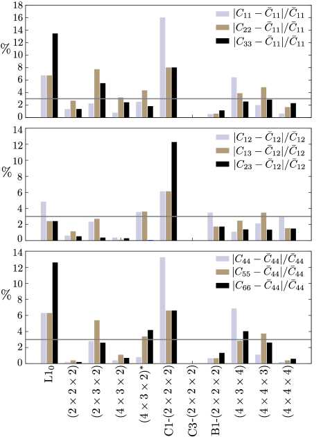
Figure 2: (Color online) Comparison of the calculated elastic tensor elements with the projected principal cubic elastic constants in Ti_0.5Al_0.5N.

In this figure the three columns for each supercell give the deviations along the three orthogonal directions, [100], [010] and [001]. One can see in the figure, where the horizontal lines show our 3% error threshold, that in the 9 dimensional space only three supercells, the $(2\times 2\times 2)$, C3-$(2\times 2\times)$ and $(4\times 4\times 4)$ give cubic elastic symmetry. Similarly to Fig. 1 the $(4\times 4\times 3)$ supercells performs very well, while the totally random $(4\times 3\times 4)$ does not. Accordingly, Fig. 2 correlates quite well with Fig. 1, namely we see the same set of structures that performing perfectly good or bad. This leads us to the conclusion that one can analyze the performance of the supercells in describing cubic elasticity within this 9 dimensional subspace, too. This means a great reduction in the computational cost, since only 9 elements have to be calculated to measure the representation of elasticity. By the way, the analysis in this 9 dimensional subspace might result in another best approximate superstructure, like in this study. Fig. 2 shows clearly, that the $(4\times 4\times 4)$ supercell results in a somewhat better representation of cubic elastic symmetry in this space.

However, this small discrepancy between the two previously performed analysis, within the full 21 and 9 dimensional spaces can be resolved by comparing the derived projected cubic elastic constants of the supercells. This comparison is shown in Fig. 3.

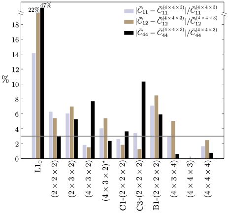
Figure 3: (Color online) The calculated projected cubic elastic constants of Ti_0.5Al_0.5N relative to the values obtained for the $(4\times 4\times 3)$ SQS model.

In Fig. 3 the relative deviations of elastic constants are plotted with respect to the values obtained for the $(4\times 4\times 3)$ SQS in correspondence with the conclusion from Fig.2. As one can see, the $(4\times 3\times 4)$ and $(4\times 4\times 4)$ supercells actually result in the same cubic elastic constants within the 3% numerical error. An interesting fact is that the values in Fig. 3 should correlate with the corresponding relative differences in Fig. 1. See, for example, the big difference between the cases of $(4\times 4\times 4)$ and B1-$(2\times 2\times 2)$. Accordingly, Fig. 3 concludes the convergency of the cubic elastic constants of Ti_0.5Al_0.5N with respect to differently shaped and sized supercell models. Accordingly, the projected cubic elastic constants can be used to predict elasticity of cubic alloys.

Since the elastic anisotropy in TiAlN alloys has a huge impact on the materials mechanical properties Tasnádi et al. (2010), an accurate prediction of the Zener’s elastic anisotropy is of a big importance. Using the projected cubic elastic constants one can derive the Zener’s elastic anisotropy via

$$\bar{A}=\frac{2\bar{C}_{44}}{\bar{C}_{11}-\bar{C}_{12}}.$$ (10)

The derived values are listed in Table 4 and plotted in Fig. 4.

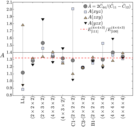
Figure 4: (Color online) Zener’s elastic anisotropy values in Ti_0.5Al_0.5N for each structural models considered in this study. The horizontal solid line shows the value of $\bar{A}$ obtained for the $(4\times 4\times 3)$ SQS.

The 3% numerical error accumulates in the nominator and results in the approximate 5% difference between the two elastic anisotropy values obtained with the best $(4\times 4\times 4)$ and $(4\times 4\times 3)$ supercells. Thus, the Zener’s elastic anisotropy in Ti_0.5Al_0.5N should have the value of A=1.40 with around 6% numerical error. Fig.4 shows not only the cubic projected elastic anisotropy values but also their variation along the three orthogonal directions, [100], [010] and [001], using the data from Table 3. For example, in the [100] direction one has $A(x,y,z)=2C_{44}/(C_{11}-C{12})$ while in the [010], $A(yzx)=2C_{66}/(C_{33}-C_{13})$. These orientational variations should vanish in case of true cubic symmetry. However, as the figure shows one may get a large orientation dependence ($\approx 55\%$, see C1-$(2\times 2\times 2)$) for a supercell being far from fulfilling cubic point symmetry. The sizes of the variations should correlate with the deviations shown in Fig. 2. Accordingly, Fig. 4 gives a similar way to analyze the performance of the supercells in modeling elasticity of cubic systems.

In the Reuss averaging method, with assumed uniform stress distribution, the strain ratio $\epsilon_{[200]}/\epsilon_{[111]}=E_{[111]}/E_{[100]}$, where $E_{[hkl]}$ denotes the directional Young’s elastic moduli, can be applied to estimate elastic anisotropy experimentally in cubic materials. Using our most accurate supercell model of $(4\times 4\times 3)$ the strain ratio $\epsilon_{[200]}/\epsilon_{[111]}$ has the value of 1.32 in Ti_0.5Al_0.5N. It is also shown in Fig.4. This value deviates from our $\bar{A}=1.40$ value less than the 6% numerical error. The elasticity of polycrystalline Ti_0.5Al_0.5N can be discussed in terms of the Reuss and Voigt bulk ($B_{\text{R}},B_{\text{V}}$) and shear moduli ($G_{\text{R}},G_{\text{V}}$) and also the derived Young’s modulus ($E_{\text{V/G}}$) and Poisson ratio ($\nu_{\text{V/G}}$),

$$B_{\text{V}}=\frac{(C_{11}+C_{22}+C_{33})+2(C_{12}+C_{13}+C{23})}{9},$$

$$G_{\text{V}}=\frac{(C_{11}+C_{22}+C_{33})-(C_{12}+C_{13}+C{23})+3(C_{44}+C_{55}+C_{66})}{15},$$

$$B_{\text{R}}=\frac{1}{(S_{11}+S_{22}+S_{33})+2(S_{12}+S_{13}+S_{23})},$$

$$G_{\text{R}}=\frac{15}{4(S_{11}+S_{22}+S_{33})-4(S_{12}+S_{13}+S_{23})+3(S_{44}+S_{55}+S_{66})},$$

$$E=\frac{9BG}{3B+G},\quad\nu=\frac{3B-2G}{6B+2G}$$ (11)

where $S_{ij}$ denotes the elastic compliances. These polycrystalline averaged quantities obtained for our the supercell $(4\times 4\times 3)$, that approximates both the randomness and cubic symmetry accurately, are summarized in Table 5.

Table 5: The polycrystalline bulk (B), shear (G), Young (E) moduli in unit of GPa and the Poisson ratio of Ti_0.5Al_0.5N obtained with the $(4\times 4\times 3)$ supercell.

B${}_{\text{V}}$	B${}_{\text{R}}$	G${}_{\text{V}}$	G${}_{\text{R}}$	E${}_{\text{V}}$	E${}_{\text{R}}$	$\nu_{\text{V}}$	$\nu_{\text{R}}$
254	254	180	174	437	425	0.21	0.22

The values clearly show the cubic requirement of $B_{\text{R}}=B_{\text{V}}$.

IV Summary

In this study we discuss the performance of superstructures, including approximate special quasirandom structure (SQS) supercells in modeling the elasticity of cubic B1 Ti_0.5Al_0.5N alloy. Though the SQS approach provides a successful scheme to model and predict the thermodynamics of alloys, the technique is not aiming to represent tensorial materials properties with symmetry. Thus, its straightforward application can not provide an unambiguous description of elasticity in random alloys.

Here, we applied a symmetry based projection technique to accurately predict the cubic elastic tensor of B1 Ti_0.5Al_0.5N alloy within the SQS approach. We derived from ab-initio calculations the closest cubic elastic tensor of B1 Ti_0.5Al_0.5N by using several supercells. With the help of these derived cubic projected elastic constants we presented a detailed analysis and comparison of differently shaped and sized supercell models in describing elasticity of a system with cubic symmetry. Thus, we accurately determined the cubic elastic constants of cubic Ti_0.5Al_0.5N. The $(4\times 4\times 3)$ supercell provided us the best model of both, randomness and elasticity, which resulted in $C_{11}=447$ GPa, $C_{12}=158$ GPa and $C_{44}=203$ GPa for the cubic elastic constants with 3% of error and $A=1.40$ for Zener’s elastic anisotropy with 6% of error.

With the help of the obtained elastic tensors, each with 21 constants, our results established the fact that supercells with good SRO parameters may include large non-cubic elastic constants and, on the contrary, supercells with bad SRO parameters might approximate cubic elastic tensor fairly accurately. We showed that using only 9 elements, $C_{11}$, $C_{22}$, $C_{33}$, $C_{12}$, $C_{13}$, $C_{23}$, $C_{44}$, $C_{55}$ and $C_{66}$ constants from the tensors, one can also adequately evaluate the supercell models and convergency of the results. We also showed that, the deviations between the three equivalent Zener-type anisotropy factors, oriented along the [100], [010] and [001] directions, confirm the same observation and establish a measure of approximate cubic symmetry.

In summary, in this study we accurately predict cubic elastic constants of B1 Ti_0.5Al_0.5N alloy and establish in general the importance of selecting proper SQS supercells with symmetry arguments to reliably model elasticity of alloys. Furthermore, we suggest the calculation of nine elastic tensor elements - $C_{11}$, $C_{22}$, $C_{33}$, $C_{12}$, $C_{13}$, $C_{23}$, $C_{44}$, $C_{55}$ and $C_{66}$, to evaluate and analyse the performance of supercells in describing elasticity of alloys.

V Acknowledgemnt

This work was supported by the SSF project Designed Multicomponent coatings, MultiFilms and the Swedish Research Council (VR). Calculations have been performed at Swedish National Infrastructure for Computing (SNIC).

Appendix A Appendix A: The atomic distributions and coordinates in the supercells

The atomic distributions and coordinates relative to the supercells lattice parameters are listed in Tables 6,7. For the atomic distributions and coordinates in C1-$(2\times 2\times 2)$, C3-$(2\times 2\times 2)$ and B1-$(2\times 2\times 2)$, see Ref.von Pezold et al. (2010).

Table 6: The internal atomic structures of the supercells in relative coordinates.

($2\times 2\times 2$)		($2\times 3\times 2$)		($4\times 3\times 2$)		($4\times 3\times 2$)
Ti	0 0 0	Ti	0 0 0	Al	0 0 0	Al	0 0 0
Al	1/2 0 0	Al	1/2 0 0	Al	1/4 0 0	Ti	1/4 0 0
Ti	0 1/2 0	Ti	0 1/3 0	Al	1/2 0 0	Al	1/2 0 0
Ti	1/2 1/2 0	Al	0 2/3 0	Ti	3/4 0 0	Ti	3/4 0 0
Al	0 0 1/2	Ti	1/2 1/3 0	Al	0 1/3 0	Ti	0 1/3 0
Ti	1/2 0 1/2	Ti	1/2 2/3 0	Ti	0 2/3 0	Al	0 2/3 0
Al	0 1/2 1/2	Al	0 0 1/2	Ti	1/4 1/3 0	Al	1/4 1/3 0
Al	1/2 1/2 1/2	Al	1/2 0 1/2	Al	1/4 2/3 0	Ti	1/4 2/3 0
		Ti	0 1/3 1/2	Ti	1/2 1/3 0	Ti	1/2 1/3 0
		Al	0 2/3 1/2	Ti	1/2 2/3 0	Ti	1/2 2/3 0
		Al	1/2 1/3 1/2	Al	3/4 1/3 0	Ti	3/4 1/3 0
		Ti	1/2 2/3 1/2	Ti	3/4 2/3 0	Al	3/4 2/3 0
				Ti	0 0 1/2	Ti	0 0 1/2
				Al	1/4 0 1/2	Ti	1/4 0 1/2
				Ti	1/2 0 1/2	Al	1/2 0 1/2
				Ti	3/4 0 1/2	Al	3/4 0 1/2
				Ti	0 1/3 1/2	Al	0 1/3 1/2
				Al	0 2/3 1/2	Ti	0 2/3 1/2
				Al	1/4 1/3 1/2	Al	1/4 1/3 1/2
				Al	1/4 2/3 1/2	Al	1/4 2/3 1/2
				Al	1/2 1/3 1/2	Ti	1/2 1/3 1/2
				Al	1/2 2/3 1/2	Ti	1/2 2/3 1/2
				Ti	3/4 1/3 1/2	Al	3/4 1/3 1/2
				Ti	3/4 2/3 1/2	Al	3/4 2/3 1/2

Table 7: The internal atomic structures of the supercells in relative coordinates (continuation).

($4\times 3\times 4$)		($4\times 4\times 3$)		($4\times 4\times 4$)
Ti	0 0 0	Al	0 0 0	Ti	0 0 0
Al	1/4 0 0	Al	1/4 0 0	Al	1/4 0 0
Ti	1/2 0 0	Al	3/4 0 0	Al	1/2 0 0
Ti	3/4 0 0	Al	0 0 1/3	Ti	3/4 0 0
Ti	0 1/3 0	Al	0 0 2/3	Ti	0 1/4 0
Ti	0 2/3 0	Al	1/4 0 1/3	Ti	0 1/2 0
Al	1/4 1/3 0	Al	1/4 0 2/3	Ti	0 3/4 0
Al	1/4 2/3 0	Al	1/2 0 1/3	Al	1/4 1/4 0
Ti	1/2 1/3 0	Al	1/2 0 2/3	Ti	1/4 1/2 0
Ti	1/2 2/3 0	Al	0 3/4 0	Ti	1/4 3/4 0
Ti	3/4 1/3 0	Al	1/4 1/4 0	Al	1/2 1/4 0
Ti	3/4 2/3 0	Al	1/2 3/4 0	Ti	1/2 1/2 0
Ti	0 0 1/4	Al	3/4 1/4 0	Ti	1/2 3/4 0
Al	0 0 1/2	Al	0 3/4 1/3	Ti	3/4 1/4 0
Al	0 0 3/4	Al	0 1/2 2/3	Ti	3/4 1/2 0
Al	1/4 0 1/4	Al	0 3/4 2/3	Al	3/4 3/4 0
Al	1/4 0 1/2	Al	1/4 1/4 1/3	Ti	0 0 1/4
Ti	1/4 0 3/4	Al	1/4 1/4 2/3	Al	0 0 1/2
Ti	1/2 0 1/4	Al	1/4 1/2 2/3	Al	0 0 3/4
Al	1/2 0 1/2	Al	1/2 1/4 1/3	Ti	1/4 0 1/4
Al	1/2 0 3/4	Al	1/2 3/4 1/3	Al	1/4 0 1/2
Al	3/4 0 1/4	Al	1/2 3/4 2/3	Ti	1/4 0 3/4
Ti	3/4 0 1/2	Al	3/4 1/4 1/3	Al	1/2 0 1/4
Ti	3/4 0 3/4	Al	3/4 1/4 2/3	Al	1/2 0 1/2
Ti	0 1/3 1/4	Ti	1/2 0.0 0	Ti	1/2 0 3/4
Al	0 1/3 1/2	Ti	3/4 0.0 1/3	Al	3/4 0 1/4
Al	0 1/3 3/4	Ti	3/4 0.0 2/3	Al	3/4 0 1/2
Ti	0 2/3 1/4	Ti	0 1/4 0	Al	3/4 0 3/4
Al	0 2/3 1/2	Ti	0 1/2 0	Ti	0 1/4 1/4
Al	0 2/3 3/4	Ti	1/4 1/2 0	Al	0 1/4 1/2
Al	1/4 1/3 1/4	Ti	1/4 3/4 0	Al	0 1/4 3/4
Al	1/4 1/3 1/2	Ti	1/2 1/4 0	Al	0 1/2 1/4
Ti	1/4 1/3 3/4	Ti	1/2 1/2 0	Ti	0 1/2 1/2
Al	1/4 2/3 1/4	Ti	3/4 1/2 0	Ti	0 3/4 1/4
Al	1/4 2/3 1/2	Ti	3/4 3/4 0	Ti	0 3/4 1/2
Ti	1/4 2/3 3/4	Ti	0 1/4 1/3	Al	0 3/4 3/4
Ti	1/2 1/3 1/4	Ti	0 1/2 1/3	Ti	1/4 1/4 1/4
Al	1/2 1/3 1/2	Ti	0 1/4 2/3	Ti	1/4 1/4 1/2
Al	1/2 1/3 3/4	Ti	1/4 1/2 1/3	Al	1/4 1/4 3/4
Ti	1/2 2/3 1/4	Ti	1/4 3/4 1/3	Ti	1/4 1/2 1/4
Al	1/2 2/3 1/2	Ti	1/4 3/4 2/3	Al	1/4 1/2 1/2
Al	1/2 2/3 3/4	Ti	1/2 1/2 1/3	Ti	1/4 1/2 3/4
Al	3/4 1/3 1/4	Ti	1/2 1/4 2/3	Ti	1/4 3/4 1/4
Ti	3/4 1/3 1/2	Ti	1/2 1/2 2/3	Al	1/4 3/4 1/2
Ti	3/4 1/3 3/4	Ti	3/4 1/2 1/3	Al	1/4 3/4 3/4
Al	3/4 2/3 1/4	Ti	3/4 3/4 1/3	Ti	1/2 1/4 1/4
Ti	3/4 2/3 1/2	Ti	3/4 1/2 2/3	Al	1/2 1/4 1/2
Ti	3/4 2/3 3/4	Ti	3/4 3/4 2/3	Ti	1/2 1/4 3/4
				Al	1/2 1/2 1/2
				Al	1/2 1/2 3/4
				Ti	1/2 3/4 1/4
				Al	1/2 3/4 1/2
				Al	1/2 3/4 3/4
				Ti	3/4 1/4 1/4
				Al	3/4 1/4 1/2
				Al	3/4 1/4 3/4
				Al	3/4 1/2 1/4
				Ti	3/4 1/2 1/2
				Al	3/4 1/2 3/4
				Ti	3/4 3/4 1/4
				Ti	3/4 3/4 1/2
				Al	3/4 3/4 3/4

Appendix B Appendix B: Elastic tensors (in GPa) of cubic TiN, AlN and Ti_0.5Al_0.5N calculated for supercells from Table 1

B.0.1 Elastic tensor of B1 TiN

$$\begin{pmatrix}617&123&123&-2&-6&-6\\ &618&123&-6&-2&-6\\ &&618&-6&-6&-2\\ &&&178&-4&-4\\ &&&&178&-4\\ &&&&&178\end{pmatrix}$$

B.0.2 Elastic tensor of B1 AlN

$$\begin{pmatrix}402&157&157&0&0&0\\ &402&157&0&0&0\\ &&402&0&0&0\\ &&&300&0&0\\ &&&&300&0\\ &&&&&300\end{pmatrix}$$

B.0.3 Elastic tensor of L1₀ structure

$$\begin{pmatrix}409&183&197&44&44&49\\ &409&197&44&44&49\\ &&332&45&45&49\\ &&&100&44&46\\ &&&&100&46\\ &&&&&120\end{pmatrix}$$

B.0.4 Elastic tensor of $(2\times 2\times 2)$ SQS

$$\begin{pmatrix}469&148&151&-3&-5&-3\\ &488&148&-3&3&-3\\ &&469&-3&-5&-3\\ &&&210&-4&-4\\ &&&&208&-4\\ &&&&&210\end{pmatrix}$$

B.0.5 Elastic tensor of $(2\times 3\times 2)$ SQS

$$\begin{pmatrix}429&173&164&2&4&6\\ &388&169&15&16&4\\ &&443&11&9&16\\ &&&187&9&8\\ &&&&203&9\\ &&&&&188\end{pmatrix}$$

B.0.6 Elastic tensor of $(4\times 3\times 2)$ SQS

$$\begin{pmatrix}436&161&160&12&11&25\\ &453&160&4&15&1\\ &&428&13&3&8\\ &&&188&12&9\\ &&&&186&9\\ &&&&&189\end{pmatrix}$$

B.0.7 Elastic tensor of $(4\times 3\times 2)^{\ast}$ SQS

$$\begin{pmatrix}477&144&155&-2&2&9\\ &445&149&-1&3&-14\\ &&474&3&-6&1\\ &&&210&0&2\\ &&&&215&1\\ &&&&&199\end{pmatrix}$$

B.0.8 Elastic tensor of C1-$(2\times 2\times 2)$ structure

$$\begin{pmatrix}385&164&164&4&4&4\\ &495&136&0&1&0\\ &&495&0&0&1\\ &&&222&3&3\\ &&&&183&2\\ &&&&&183\end{pmatrix}$$

B.0.9 Elastic tensor of C3-$(2\times 2\times 2)$ structure

$$\begin{pmatrix}462&156&156&6&6&6\\ &462&156&6&6&6\\ &&462&6&6&6\\ &&&182&6&6\\ &&&&182&6\\ &&&&&182\end{pmatrix}$$

B.0.10 Elastic tensor of B1-$(2\times 2\times 2)$ structure from Ref.von Pezold et al. (2010).

$$\begin{pmatrix}481&139&147&-1&-4&-2\\ &482&147&-4&-1&-2\\ &&473&-1&-1&-2\\ &&&214&-1&-1\\ &&&&214&-1\\ &&&&&201\end{pmatrix}$$

B.0.11 Elastic tensor of $(4\times 3\times 4)$ SQS

$$\begin{pmatrix}431&148&153&-2&25&21\\ &478&148&-11&-10&-16\\ &&472&9&-11&5\\ &&&216&3&0\\ &&&&196&-1\\ &&&&&194\end{pmatrix}$$

B.0.12 Elastic tensor of $(4\times 4\times 3)$ SQS

$$\begin{pmatrix}456&161.05&152&1&2&4\\ &425&160&7&4&1\\ &&460&3&1&9\\ &&&201&3&5\\ &&&&211&3\\ &&&&&198\end{pmatrix}$$

B.0.13 Elastic tensor of $(4\times 4\times 4)$ SQS

$$\begin{pmatrix}457&149&156&-2&14&19\\ &462&156&-11&-3&-16\\ &&444&17&-5&1\\ &&&202&0&-1\\ &&&&203&-1\\ &&&&&200\par\end{pmatrix}$$

References

- (1) A. Hörling, L. Hultman, M. Odén, J. Sjölén, and L. Karlsson, Surf. Coat. Technol. 191, 384 (2002).
- Alling et al. (2007) B. Alling, A. Ruban, A. Karimi, O. Peil, S. Simak, L. Hultman, and I. Abrikosov, Phys. Rev. B 75 045123 (2007).
- Mayrhofer et al. (2006) P. Mayrhofer, D. Musics, and J.M. Schenider, Appl. Phys. Lett. 88 071922, (2006).
- Alling et al. (2008) B. Alling, A. Karimi, L. Hultman, and I. A. Abrikosov, Appl. Phys. Lett. 92, 071903 (2008).
- Alling et al. (2009) B. Alling, M. Odén, L. Hultman, and I. A. Abrikosov, Appl. Phys. Lett. 95, 181906 (2009).
- Lind et al. (2003) H. Lind, R. Forsén, B. Alling, N. Ghafoor, F. Tasnádi, M.P. Johansson, I.A. Abrikosov, and M. Odén, Appl. Phys. Lett. 99, 091903 (2011).
- Tasnádi et al. (2010) F. Tasnádi, I. A. Abrikosov, L. Rogström, J. Almer, M. P. Johansson, and M. Odén, Appl. Phys. Lett. 97, 231902 (2010).
- Abrikosov et al. (2010) I.A. Abrikosov, A. Knutsson, B. Alling, F. Tasnádi, H. Lind, L. Hultman, and M. Odén, Materials 4, 1599 (2011).
- Ruban and Abrikosov (2008) A. V. Ruban and I. A. Abrikosov, Rep. Prog. Phys. 71, 046501 (2008).
- Liu et al. (2005) J. Liu, A. van de Walle, G. Ghosh, and M. Asta, Phys. Rev. B 72 144109 (2005).
- van de Walle (2008) A. van de Walle, Nat. Mater. 7, 455 (2008).
- Asta et al. (1991) M. Asta, C. Wolverton, D. de Fontaine, and H. Dreyssé, Phys. Rev. B 44, 4907 (1991).
- Zunger et al. (1990) A. Zunger, S.-H. Wei, L. Ferreira, and J. Bernard, Phys. Rev. Lett. 65, 353 (1990).
- Tasnádi et al. (2010) F. Tasnádi, B. Alling, C. Höglund, G. Wingqvist, J. Birch, L. Hultman, and I. A. Abrikosov, Phys. Rev. Lett. 104, 137601 (2010).
- Wingqvist et al. (2010) G. Wingqvist, F. Tasnádi, A. Zukauskaite, J. Birch, H. Arwin, and L. Hultman, Appl. Phys. Lett. 97, 112902 (2010).
- Mayrhofer et al. (2006) P. H. Mayrhofer, D. Music, and J. M. Schneider, J. Appl. Phys. 100, 094906 (2006).
- Tasnádi et al. (2009) F. Tasnádi, I. A. Abrikosov, and I. Katardjiev, Appl. Phys. Lett. 94, 151911 (2009).
- Mäder and Zunger (1995) K. Mäder and A. Zunger, Phys. Rev. B 51, 10462 (1995).
- Bernardini et al. (2001) F. Bernardini, andV. Fiorentini, Phys. Rev. B 64, 085207 (2001).
- von Pezold et al. (2010) J. von Pezold, A. Dick, M. Friák, and J. Neugebauer, Phys. Rev. B 81 (2010).
- Cowley (1950) J. Cowley, Phys. Rev. 77, 669 (1950).
- Metropolis et al. (1953) N. Metropolis, A. W. Rosenbluth, M. N. Rosenbluth, A. H. Teller, and E. Teller, J. Chem. Phys. 21, 1087 (1953).
- Vanderbilt (1990) D. Vanderbilt, Phys. Rev. B 41, 7892 (1990).
- Giannozzi et al. (2009) P. Giannozzi, S. Baroni, N. Bonini, M. Calandra, R. Car, C. Cavazzoni, D. Ceresoli, G. L. Chiarotti, M. Cococcioni, I. Dabo, et al., J. of Phys.: Condens. Matter 21, 395502 (2009).
- Perdew et al. (1996) J. P. Perdew, K. Burke, and M. Ernzerhof, Phys. Rev. Lett. 77, 3865 (1996).
- Monkhorst and Pack (1976) H. Monkhorst and J. Pack, Phys. Rev. B 13, 5188 (1976).
- Chen et al. (2003) K. Chen, L.R. Zhao, J. Rodgers, and J.S. Tse, J. Phys. D: Appl. Phys 36, 2725 (2003).
- Wentzcovitch et al. (1993) R. M. Wentzcovitch, J. L. Martins, and G. D. Price, Phys. Rev. Lett. 70, 3947 (1993).
- Nye (1985) J. F. Nye, Physical Properties of Crystals: Their Representation by Tensors and Matrices (Oxford University Press, USA, 1985), ISBN 0198511655.
- Vitos (2010) L. Vitos, Computational Quantum Mechanics for Materials Engineers: The EMTO Method and Applications (Engineering Materials and Processes) (Springer, 2010), ISBN 1849966850.
- Browaeys and Chevrot (2004) J. T. Browaeys and S. Chevrot, Geophys. J. Int. 159, 667 (2004).
- Moakher and Norris (2006) M. Moakher and A. N. Norris, J. Elasticity 85, 215 (2006).