A three dimensional investigation of two dimensional orbits

Abstract

Orbits in the principal planes of triaxial potentials are known to be prone to unstable motion normal to those planes, so that three dimensional investigations of those orbits are needed even though they are two dimensional. We present here an investigation of such orbits in the well known logarithmic potential which shows that the third dimension must be taken into account when studying them and that the instability worsens for lower values of the forces normal to the plane. Partially chaotic orbits are present around resonances, but also in other regions. The action normal to the plane seems to be related to the isolating integral that distinguishes regular form partially chaotic orbits, but not to the integral that distinguishes partially from fully chaotic orbits.

1 Introduction

Stellar systems are clearly three-dimensional (3D) in configuration space. Nevertheless, since the study of two-dimensional (2D) systems is much easier than that of 3D ones, both analiytically and numerically, it is tempting in many instances to resort to the 2D approach. Standard examples are investigations of 2D orbits in the equatorial plane of disk galaxies or in the principal planes of elliptical ones. The risks of resorting to this simplification in the case of elliptical galaxies were emphasized by MF96 , but their words of caution may be valid for disk galaxies as well. The main problem is that orbits in the principal planes are often unstable to perturbations out of the plane, so that such instability would not be detected in 2D studies and, as a result, orbits that a full 3D study would reveal as chaotic might appear as regular in a 2D investigation. Another investigation of orbits in triaxial models with weak cusps by FM97 also found many cases of instability normal to the principal planes. Besides, the more recent investigation of Aetal07 puts the original warning of MF96 in an even more general context.

There is a mathematical peculiarity that makes a full 3D study of 2D orbits in the principal planes particularly interesting. Let us assume that we choose the $(x,y)$ plane and that we adopt initial conditions $x=x_{0}$, $y=y_{0}$, $z=0$, $V_{x}=V_{x0}$, $V_{y}=V_{y0}$ and $V_{z}=0$. Since both $z$ and $V_{z}$ are exactly zero and there is no rounding off error in the numerical representation of that number, the time derivatives of $z$ and $V_{z}$ in the equations of motion will remain always equal to zero and the orbit will remain forever on the $(x,y)$ plane, even if it is unstable in the $z$ direction. Nevertheless, if the variational equations are computed at the same time as the orbit, they will clearly reveal how an infinitesimally small departure from that orbit will exponentially grow and, thus, the chaotic nature of the orbit. Therefore, a 3D investigation of 2D orbits on the principal planes of a triaxial potential computing the Lyapunov exponents via the variational equations seems warranted.

Moreover, we have emphasized several times over the past decade (e.g. Muz03 , MM04 , MCW05 , AMNZ07 , MNZ09 ) the importance of distinguishing between partially and fully chaotic orbits in dynamical studies of stellar systems. The sole isolating integral of fully chaotic orbits is the energy, while partially chaotic orbits obey an additional isolating integral or pseudo integral. The Lyapunov exponents offer a simple way to distinguish these orbits because, due to the conservation of phase space volume in Hamiltonian systems, these exponents come in pairs, one positive and one negative, with the same absolute value. Besides, energy conservation in autonomous systems ensures that one of those pairs has zero absolute value, and each additional isolating integral results in another pair of exponents equal to zero. Therefore, in a 3D potential we may have all three pairs of exponents equal to zero (regular orbit), only one pair not equal to zero (partially chaotic orbit), or two non–zero pairs of Lyapunov exponents (fully chaotic orbit). In 2D potentials, instead, we can only have regular (two null pairs of exponents) or partially chaotic orbits (one null and one non–null pairs).

There has been some discussion recently about whether the partially chaotic orbits are simply those that belong in the stochastic layer surrounding resonances around regular orbits (NPM07 ) or they cover more extended regions of phase space (AMNZ07 ). Now, 2D orbits can be either regular or partially chaotic, but not fully chaotic because they can obey two integrals of motion only or, alternatively, they have only four Lyapunov exponents instead of the six of 3D orbits. Thus, we can expect that an investigation of orbits close to the main planes of a triaxial potential may shed some light on the nature of the partially chaotic orbits.

The logarithmic potential (see, e.g. BT08 ) has been frequently used for 2D studies (see, e.g. MS89 , PL96 , CA98 , FB01 ), so that it may be interesting to check how much it is affected by instabilities out of the plane. Besides, it has a simple mathematical expression that allows a reasonably fast computation of all the Lyapunov exponents. Therefore, we decided to perfom an investigation of 2D orbits on the principal planes of the 3D logarithmic potential. The next section describes our method and the third one presents our results which are then discussed in the fourth section.

2 Method

Our investigation is based on the comparison of the chaoticity of orbits moving in a 2D potential with that of orbits moving in a 3D potential. Two possibilities are considered in the latter case: 1) Initial conditions very close to one of the principal planes of symmetry, but not exactly on it; 2) Initial conditions precisely on a principal plane. The reason for considering these two possibilities is that, as indicated above, in the second case the orbit is forced to remain on the plane for mathematical reasons, even if it is unstable perpendicularly to the plane. In order to recognize regular from chaotic, and partially from fully chaotic orbits, we compute all the Lyapunov exponents corresponding to the case in question, i.e., four in the 2D, and six in the 3D cases.

As indicated, we adopted the 3D logarithmic potential:

$$\Phi(\vec{x})={V_{0}^{2}\over 2}\ln\left({R_{\rm c}^{2}}+{x^{2}\over a^{2}}+{y^{2}\over b^{2}}+{z^{2}\over c^{2}}\right),$$ (1)

where $V_{0}$, $R_{\rm c}$, $a$, $b$ and $c$ are constants. The equipotentials are ellipsoids whose semiaxes are proportional to $a$, $b$ and $c$. For the 2D case we simply omitted the $z$ coordinate, both in the equations of motion and in the variational equations.

In order to compare corresponding orbits in the 2D and 3D cases, we chose a fixed set of initial conditions. We took 90 equidistant points along each axis of the $\{y,V_{y}\}$ plane defined by $E=0$ and $x=z=V_{z}=0$, where $E$ is the energy of the orbit. The allowed region on this plane is defined by the condition $V_{x}^{2}>0$. The symmetries of the potential allowed us to restrict our study to the region $y>0$, $V_{x}>0$ and $V_{y}>0$. We then set $V_{0}=1$, $R_{\rm c}=0.01$, $a=1$ and $b=0.7$ and we picked up each of the resulting $(y,V_{y})$ pairs as initial conditions whenever they allowed to obtain $E=0$ with a real value of $V_{x}$.

We integrated the equations of motion and the corresponding variational equations with a double precision Runge-Kutta-Fehlberg algorithm of order 7, with Cash-Karp coefficients PTVF86 . In order to obtain information about the degree of chaoticity of the orbits, the full set of Lyapunov exponents was computed for each orbit using the well-known algorithm developed by BGGS80a , BGGS80b . To this end, the six necessary variational initial conditions were obtained by perturbing the original ones along each of the six axes of the phase space. The orbits were integrated over $t=10,000$ time units (t.u.), which corresponds to a number of orbital periods between 1500 and 3500, approximately. The energy is conserved to better than $3\times 10^{-10}$ in all cases, and better than $5\times 10^{-11}$ in most cases.

As is well known, the Lyapunov exponents, being defined as values of a certain function $f(t)$ when $t\to\infty$, cannot be computed directly from a numerical experiment. Instead, the Lyapunov characteristic numbers (LCNs) are used, that is, the values of $f(t)$ at finite times, the validity of this approximation resting on the reasonable assumption that the LCNs will tend to the Lyapunov exponents as $t\to\infty$. However, this raises the question of what LCN value will be considered the equivalent of a zero value of the corresponding Lyapunov exponent. To answer it we present in Fig. 1 (left) a plot of the largest LCN, LCN_max, versus the second largest one, LCN_int for the case with $c=0.5$ (see below). The figure clearly shows a cluster of points near the left lower corner that corresponds to regular orbits and another cluster near the right upper corner that corresponds to the fully chaotic orbits. Besides, there is an horizontal band that extends over most of the middle part of the plot that corresponds to the partially chaotic orbits. The horizontal and vertical lines at ${\rm LCN}=0.00155$ show the chosen limiting value for the LCNs. No doubt, that limiting value is only approximate and of statistical nature, since a few orbits with LCNs slightly larger (smaller) than the limiting value might actually be regular (chaotic), but the figure shows that it clearly separates the three different types of orbits. The right part of Fig. 1 shows the same plot as the left part, but using an integration time of 50,000 t.u. The limiting value is lower now (about ${\rm LCN}=0.00040$) but, except for that fact, the general aspect of both plots is essentially the same. Of course, some sticky orbits that appear as regular on the left figure reveal their true chaotic nature on the right one, but the effect is small (the number of regular orbits falls from $29.2\%$ to $28.7\%$ only), so that the chosen integration limit of 10,000 t.u. is most adequate for the present investigation.

Figure 1: Largest Lyapunov characteristic numbers (LCN_max) vs. intermediate Lyapunov characteristic numbers (LCN_int) for the $c=0.50$ potential studied. The integration time was 10,000 t.u. for the left plot and 50,000 t.u. for the right one. The limiting value ${\rm LCN}=0.00155$ is marked with straight lines as a reference on the left plot; the corresponding limiting value ${\rm LCN}=0.00040$ is marked on the right one.

With these tools, we integrated orbits in several potentials with the abovementioned fixed values of $V_{0}$, $R_{\rm c}$, $a$ and $b$. In the 2D case nothing more is needed. In the 3D case, however, the parameter $c$ is still undefined. We took several values of $c$ in the interval $(0,1]$. Thus, the series of studied potentials goes from very flattened and similar to the 2D case, through axisymmetric prolate (when $c=0.7$), to axisymmetric oblate (when $c=1$). This allowed us to study whether and when the third dimension, although not seen by the star, plays a role in its regularity or chaoticity.

3 Numerical experiments and results

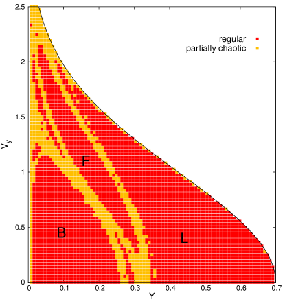
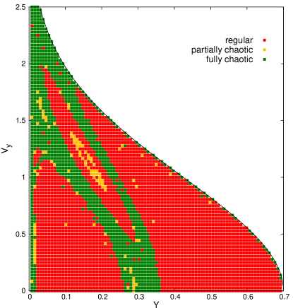
Figure 2: Left: Regular or partially chaotic character of orbits in the 2D potential model, each of which is launched with initial conditions $E=x=0$ and $(y,V_{y})$ given by the coordinates of the corresponding point on the plot. White regions correspond to regular orbits; letters into the plot refer to the main regular families (see text) and the limiting ($V_{x}=0$) curve is also shown. Right: Regular, partially or fully chaotic character of orbits with the same initial conditions of the left figure, plus $z=10^{-6},V_{z}=0$, in the 3D potential model with $c=0.30$.

We first reproduced (Fig. 2, left) the well-known orbital content of the 2D potential model MS89 .

As indicated before, the only chaotic orbits here are the partially chaotic ones and the connected region of those orbits, i.e., those having the energy as the only isolating integral of motion, is clearly seen. The regular orbits are separated into disjoint regions, each one hosting a different family spawned by a specific mother closed orbit. Although we do not need to specify the families for the purposes of the present paper, we will mention the main ones here to be able to identify the regions of the plot later on. The region marked ”L” in Fig. 2 (left) is occupied by loop orbits, i.e., regular orbits in which the frequencies of greatest amplitude along each axis are in a 1:1 ratio. The ”B” region in the figure corresponds to banana orbits, with a 2:1 ratio between the abovementioned frequencies. Finally, the region with an ”F” is filled with fish orbits, with a 3:2 ratio. (It is worth noticing that these rational ratios are not ratios between the fundamental frequencies of the corresponding orbital tori.)

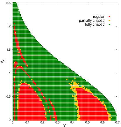
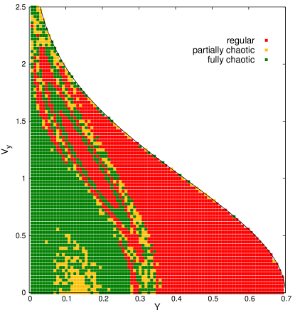
Figure 3: Left: Regular, partially or fully chaotic character of orbits in the 3D potential model with $c=0.50$. Right: Regular, partially or fully chaotic character of orbits in the 3D potential model with $c=0.695$.

Next we integrated orbits in the 3D potential for different $c$ values. We used the same initial conditions as for the 2D potential, plus $z=10^{-6},V_{z}=0$. For small $c$ values, there is no much difference with the 2D results shown in Fig. 2 (left), e.g., barely 4 points switch from partially to fully chaotic for $c=0.05$, and that number rises only to 42 points for $c=0.20$. As the value of $c$ is increased further, however, more partially chaotic orbits switch to fully chaotic and a few regular orbits switch to partially chaotic. The right panel of Fig. 2 presents the results for $c=0.30$, when all the partially chaotic orbits have turned to fully chaotic and a small island of partially chaotic orbits has appeared inside the regular region corresponding to the fish orbits. As we continued increasing $c$ the region covered by fully chaotic orbits extends its area and other regions of partially chaotic orbits appear as shown by Fig. 3 (left) that presents the results for $c=0.50$. Nevertheless, it is obvious that the situation should change when approaching $c=b=0.70$, because then we have a prolate potential that conserves the component of the angular momentum parallel to the major axis and, thus, no fully chaotic orbits can be present. In fact, the corresponding figure for that case is essentially the same as the one presented in Fig. 2 (left) for the 2D case. But, very close to $c=0.70$, the situation is different, as shown in Fig. 3 (right), corresponding to $c=0.695$ and Fig. 4 (left), for the case $c=0.705$. In both cases, most of the initial conditions result in chaotic orbits, mainly fully chaotic ones, but the regular orbits that originate from initial conditions on the $(y,V_{y})$ plane, when $y$ is still the smallest axis ($c=0.695$) tend to be loops, while when $y$ becomes the intermediate axis those regular orbits are mainly bananas. This result is quite natural, because there are no stable tubes around the intermediate axis.

As $c$ is increased even further the bananas last ”island of resistance” shrinks and the few scattered partially chaotic orbits in the (former) tubes region transform in fully chaotic orbits, as shown by Fig. 4 (right). As we approach the value $c=1.00$, chaos recedes because for that value we get again a rotationally symmetric (prolate) potential, and we get again a plot similar to that of Fig. 2 (left).

We have already mentioned that, had we taken $z=0$ instead of $z=10^{-6}$ in the initial conditions, the orbits could have not left the $(x,y)$ plane, but that the chaotic character would be revealed anyway thanks to the variational equations. The cases with $z=0$ for $c=0.500,0.695,0.705$ and $0.800$ are shown in Figs. 5, left and right, and 6, left and right, respectively. Comparison with the corresponding figures obtained with an initial value $z=10^{-6}$ shows that the stochastic layers surrounding the main resonances are always fully chaotic for those $c$ values. Those regions only remained almost completely partially chaotic for low $c$ values (e.g., $c=0.05$ or $c=0.20$), for both initial $z$ values. When we reach $c=0.30$, the plot for $z=0$ (not shown) does not differ much from that for $z=10^{-6}$ shown in Fig. 2 (right): There are only a few more partially chaotic, rather than fully chaotic, orbits in the regions of the former minor resonances.

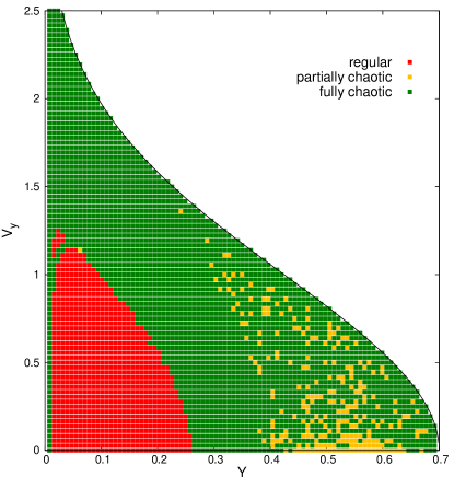
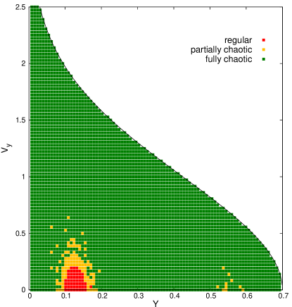
Figure 4: Left: Regular, semi-chaotic or chaotic character of orbits in the 3D potential model with $c=0.705$. Right: the same, for the case $c=0.800$.

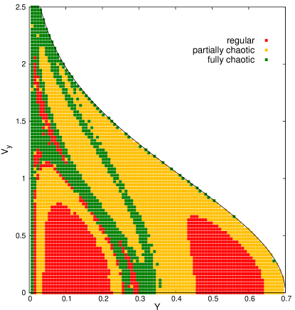
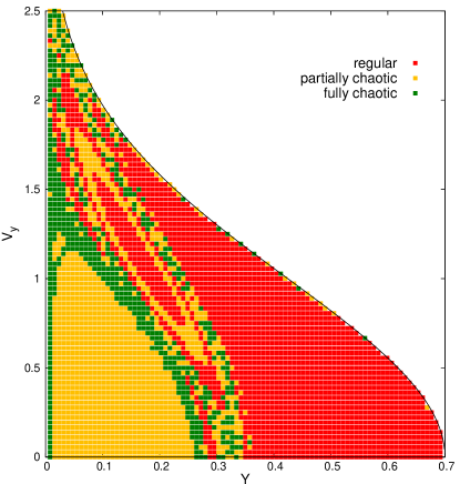
Figure 5: Left: Regular, semi-chaotic or chaotic character of orbits in the 3D potential model with $c=0.500$ when $z=0$. Right: the same, for the case $c=0.695$.

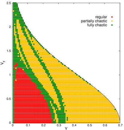
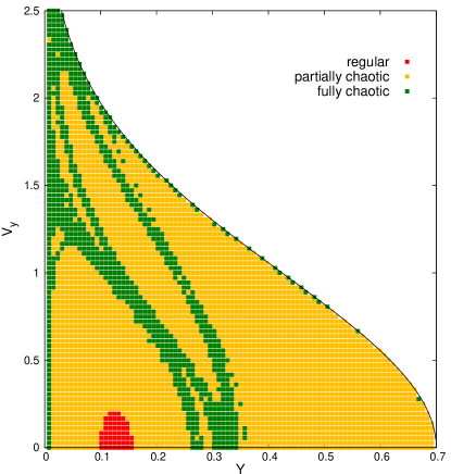
Figure 6: Left: Regular, semi-chaotic or chaotic character of orbits in the 3D potential model with $c=0.705$ when $z=0$. Right: the same, for the case $c=0.800$.

4 Discussion

Our results confirm that, even for such a simple and well studied potential as is the logarithmic one, 2D studies of the orbits in the principal symmetry planes fail to reveal the chaotic nature of many orbits. A comparison of the 2D results shown in Fig. 2 (left) with the 3D results shown in all the other figures reveals that most of the regular orbits in the 2D study become either partially or fully chaotic in the 3D cases and that most of the 2D partially chaotic orbits become fully chaotic in the 3D investigation. The motions in the equatorial plane of very flat systems (e.g., $c=0.05$ or $c=0.20$) seem to be the least affected ones by the third dimension, and the reason is easy to understand. The $x$, $y$ and $z$ accelerations are proportional, respectively, to $x/a^{2}$, $y/b^{2}$, $z/c^{2}$ so that, all other things been equal, smaller values of $c$ imply a much stronger force normal to the principal plane and, therefore, a more stable motion in that direction. It is interesting to note that, albeit for a different model, FM97 also found that the stability of $(x,y)$ banana orbits improves for lower $c/a$ values (see, e.g., their Figs. 7 and 8).

Regarding the nature of partially chaotic orbits, we notice that both possibilities indicated in the Introduction can indeed take place. We notice what clearly seems to be a chaotic layer made up of partially chaotic orbits around the 1:1 loop resonance in Fig. 3 (left) and around the 2:1 banana resonance in Fig. 4 (right); there is even a mixture of partially and fully chaotic orbits around the 3:2 fish resonance in Fig. 3 (right). Alternatively, there is a connected area dominated by partially chaotic orbits inside the 3:2 fish resonance in Fig. 2 (right), right in the middle of a region dominated by regular orbits, and another region partially connected and partially scattered of partially chaotic orbits in the middle of the fully chaotic domain in Fig. 4 (left).

Comparing the results obtained with the initial value $z=0$ with those with $z(t=0)=10^{-6}$ we notice that essentially all the orbits that are regular in one case are also regular in the other, so that the two isolating integrals that they obey, besides energy, should be the same. For partially chaotic orbits, instead, the story is different. A small fraction of those that appear in the $z=0$ cases, remain as partially chaotic when $z(t=0)=10^{-6}$, but the bulk of the partially chaotic orbits of the former case turn into fully chaotic orbits in the latter one. Clearly, the isolating integral that sustains their partially chaotic character when $z=0$ is destroyed when we let the orbit separate from the principal plane of symmetry. Besides, such integral is not valid everywhere because, except for cases with very low $c$ values, the connected region in-between resonances is dominated by fully chaotic orbits, irrespectively of whether the orbit remains in the main plane or not.

We may explore a little further the effect of the $z$ coordinate accepting that, at least for small $z$ values, the $z$ motion should be oscillatory or near oscillatory. Therefore, the additional isolating integral could be the $z$-action or some related function. To check this, we computed for each orbit the action

$$J_{z}={H\over\omega_{z}}={{1\over 2}V_{z}^{2}+{V_{0}^{2}\over 2c^{2}}{z^{2}\over R_{\rm c}^{2}+x^{2}/a^{2}+y^{2}/b^{2}}\over{V_{0}\over c\sqrt{R_{\rm c}^{2}+x^{2}/a^{2}+y^{2}/b^{2}}}},$$ (2)

where $\omega_{z}$ is the frequency of the $z$ motion computed by equating the $z$-acceleration of the potential to that of an harmonic oscillator when $z\ll 1$, and $H$ is the harmonic oscillator Hamiltonian resulting from it. It turned out that this quantity was not conserved for partially chaotic orbits, e.g., for the case $c=0.3$, we found that all partially chaotic orbits had $\log_{10}|J_{z\ {\rm final}}-J_{z\ {\rm initial}}|\in(-3,6)$ (we don’t normalize because $J_{z}\simeq 0$). Nevertheless, for the same $c=0.3$ case, all regular orbits have $\log_{10}|J_{z\ {\rm final}}-J_{z\ {\rm initial}}|\in(-12,-6)$, so that $J_{z}$, or some quantity related to it, is very likely the isolating integral that distinguishes regular from partially chaotic orbits in this case. The conservation of $J_{z}$ worsens as $c$ grows, however, so that for larger $c$ values regular orbits should obey a different isolating integral.

Therefore, our main conclusions are: 1) 3D studies are definitely necessary to investigate the stability of (apparently) 2D orbits; 2) Instability normal to the planes of symmetry worsens for lower values of the force normal to the plane (i.e., larger $c$ values in the case of the logarithmic potential); 3) We find partially chaotic orbits both in some stochastic layers around resonances and in other regions (which may be coherent or not); 4) Although the isolating integral, or pseudo integral, that distinguishes partially from fully chaotic orbits in the cases investigated might depend on the separation from the main plane ($z$), it is not related to the action normal to the plane; 5) The isolating integral, or pseudo integral, that distinguishes regular from partially chaotic orbits, instead, seems to be related to the action normal to the plane, at least for low $c$ values.

- (1) Adams, F.C., Bloch, A.M., Butler, S.C., Druce, J.M., and Ketchum, J.A., Orbital instabilities in a triaxial cusp potential, ApJ, 670, 1027-1047 (2007)
- (2) Aquilano, R.O., Muzzio, J.C., Navone, H.D. and Zorzi, A.F., Orbital structure of self–consistent triaxial stellar systems, Celest. Mech. Dynam. Astron., 99(4), 307–324 (2007)
- (3) Benettin, G., Galgani, L., Giorgilli, A., and Strelcyn, J.-M., Lyapunov characteristic exponents for smooth dynamical systems and for Hamiltonian systems; A method for computing all of them. Part 1: theory, Meccanica, March, 9-20 (1980).
- (4) Benettin, G., Galgani, L., Giorgilli, A., and Strelcyn, J.-M., Lyapunov characteristic exponents for smooth dynamical systems and for Hamiltonian systems; A method for computing all of them. Part 2: Numerical application, Meccanica, March, 21-30 (1980).
- (5) Binney J., Tremaine S., Galactic Dynamics, Princeton University Press, Princeton, NJ (2008)
- (6) Carpintero, D.D., Aguilar, L.A., Orbit classification in arbitrary 2D and 3D potentials, MNRAS, 298(1), 1–21 (1998)
- (7) Fridman, T., and Merritt, D., Periodic orbits in triaxial galaxies with weak cusps, AJ, 114, 1479-1487 (1997)
- (8) Fulton, E.E., and Barnes, J.E., A simple algorithm for orbit classification, MNRAS, 321, 507-514 (2001)
- (9) Maffione, N.P., Darriba, L.A., Cincotta, P.M., and Giordano, C.M., A comparison of different indicators of chaos based on the deviation vectors: application to symplectic mappings, Celest. Mech. Dynam. Astron., 111, 285-397 (2011)
- (10) Merritt, D., and Fridman, T., Triaxial galaxies with cups, ApJ, 460, 136-162 (1996)
- (11) Miralda-Escudé, J., and Schwarzschild, M., On the orbit structure of the logarithmic potential, ApJ, 339, 752-762 (1989)
- (12) Muzzio, J.C., Chaos in elliptical galaxies, Bol. Asoc. Argentina Astron., 45, 69 (2003)
- (13) Muzzio, J.C., Carpintero, D.D. and Wachlin, F.C., Spatial structure of regular and chaotic orbits in a self-consistent triaxial stellar system, Celest. Mech. Dynam. Astron., 91(1–2), 173–190 (2005)
- (14) Muzzio, J.C. and Mosquera, M.E., Spatial structure of regular and chaotic orbits in self-consistent models of galactic satellites, Celest. Mech. Dynam. Astron., 88(4), 379–396 (2004)
- (15) Muzzio, J.C., Navone, H.D. and Zorzi, A.F., Orbital structure of self–consistent triaxial stellar systems, Celest. Mech. Dynam. Astron., 99(4), 307–324 (2009)
- (16) Papaphilippou, Y., Laskar, J.D., Frequency map analysis and global dynamics in a galactic potential with two degrees of freedom, A&A, 307, 427–449 (1996)
- (17) Press, W.H., Teukolsky, S.A., Vetterling, W.T., and Flannery, B.P., Numerical Recipes in FORTRAN, Cambridge Univ. Press, Cambridge (1992)