Non-linear Compton scattering of ultrahigh-intensity laser pulses

Abstract

We present results for the photon spectrum emitted in non-linear Compton scattering of pulsed ultra-strong laser fields off relativistic electrons for intensities up to $a_{0}\gtrsim 100$ and pulse lengths of a few laser cycles. At ultrahigh laser intensity, it is appropriate to average over the sub-structures of the differential photon spectrum. Supplementing this procedure with a stationary phase approximation one can evaluate the total emission probability. We find the photon yield in pulsed fields to be up to a factor of ten larger than results obtained from a monochromatic wave calculation.

I Introduction

The ongoing progress in laser technology has opened an avenue towards studying strong-field QED effects in ultra-intense laser fields. Presently, the strongest available laser systems have a few petawatts, with a focused peak intensity in the order of $I=10^{22}\,\rm W/cm^{2}$ Yanovsky et al. (2008). In the near future, the high-intensity frontier will be pushed forward with ELI ELI exceeding $I=10^{24}\,\rm W/cm^{2}$, eventually. A Lorentz- and gauge-invariant dimensionless parameter characterizing the intensity is given by $a_{0}^{2}=7.9\times 10^{-19}I[{\rm W/cm^{2}}]\lambda^{2}[{\rm\mu m}]$ Salamin et al. (2006) where $I[{\rm W/cm^{2}}]$ is the laser intensity in $\rm W/cm^{2}$ and $\lambda[{\rm\mu m}]$ denotes the laser wavelength in $\rm\mu m$. Thus, values of $a_{0}$ of several hundreds can be reached in the near future.

Among other topics, the formation of QED avalanches has been discussed recently Fedotov et al. (2010); Bell and Kirk (2008) in ultra-intense laser fields, where a seed-particle leads to the formation of a cascade by consecutive photon-emission via non-linear Compton scattering and subsequent pair-production processes. Here, we focus on the non-linear Compton scattering process in laser fields with $a_{0}\gg 1$ with emphasis on finite-pulse envelope effects. The Compton process has been studied for moderately strong laser pulses $a_{0}=\mathcal{O}(1)$ both within classical electrodynamics as non-linear Thomson scattering Krafft (2004); Gao (2004); Hartemann et al. (1996); Heinzl et al. (2010a) as well as in quantum electrodynamics Narozhnyĭ and Fofanv (1996); Boca and Florescu (2009); Seipt and Kämpfer (2010); Mackenroth and Di Piazza (2011). In $a_{0}=\mathcal{O}(1)$ laser pulses, with a duration of several cycles of the carrier wave, the non-linear Compton spectrum has interesting structures with many subpeaks per harmonics, which may be verified experimentally with present technology Heinzl et al. (2010a); Seipt and Kämpfer (2011). We present here a method for calculating energy-averaged photon emission spectra for $a_{0}\gg 1$ laser pulses.

Our paper is organized as follows: In section II we evaluate the matrix element for non-linear Compton scattering. In section III we use this matrix element to calculate the emission probability, presenting our result for the phase-space averaged photon yield. In section IV we present our numerical results before concluding in section V. In appendix A we comment on the slowly varying envelope approximation. We derive an exact expression for the non-linear phase including a carrier envelope phase which has the slowly varying envelope approximation an a limit. Finally, in appendix B we have collected details on the stationary phase approximation, which is at the heart of our approach.

II Matrix Element for non-linear Compton scattering

II.1 Basic Relations

The $S$ matrix element for non-linear Compton scattering — where an electron with momentum $p$ emits a single photon with momentum $k^{\prime}$ and leaves the interaction region with momentum $p^{\prime}$ — in the Furry picture is

$$S_{fi}=-ie\int d^{4}x\overline{\Psi}_{p^{\prime}}(x)\not{\epsilon}^{\prime}\Psi_{p}(x)\frac{e^{ik^{\prime}\cdot x}}{\sqrt{2\omega^{\prime}}},$$ (1)

where the Volkov state $\Psi_{p}(x)$ Volkov (1935) is a solution of the homogeneous Dirac equation in an external classical electromagnetic plane-wave background field with four-potential $A^{\mu}(\phi)$,

$$(i\not{\partial}-e\not{A}(\phi)+m)\Psi_{p}(x)=0.$$ (2)

The Volkov solution reads

$$\Psi_{p}(x) = \exp\{-ip\cdot x-if_{p}(x)\}\left[1+\frac{e}{2k\cdot p}\not{k}\not{A}(x)\right]\frac{u_{p}}{\sqrt{2p^{0}}}$$ (3)

where the non-linear phase function is

$$f_{p}(x) = \frac{1}{2k\cdot p}\int\limits_{0}^{\phi}d\phi^{\prime}\big{[}2ep\cdot A(\phi^{\prime})-e^{2}A^{2}(\phi^{\prime})\big{]}.$$ (4)

In light-cone coordinates, e.g. $x_{\pm}=x^{0}\pm x^{3}$, $\mathbf{x}_{\perp}=(x^{1},x^{2})$ and $\mathbf{x}=(x_{+},\mathbf{x}_{\perp})$ for the spatio-temporal coordinates, the laser four-momentum $k$ has only one component which we choose to be $k_{-}$. We also define a special reference frame (s.r.f.) in which the electron is initially at rest, i.e. it has four-momentum $p=(m,0,0,0)$. Assuming a head-on collision of the electrons with the laser pulse, the laser frequency in the s.r.f. is $\omega=(\sqrt{\gamma_{0}^{2}-1}+\gamma_{0})\omega_{0}$, where $\omega_{0}$ ($\gamma_{0}$) is the laser frequency (Lorentz factor of the electron) in the laboratory system. For the vector potential $A^{\mu}$ we employ a transverse plane wave, modified by an envelope function $g$ with pulse length parameter $\tau$,

$$A^{\mu} = A_{0}\,g(\phi/\tau)\,(\epsilon_{1}^{\mu}\cos\xi\cos\phi+\epsilon_{2}^{\mu}\sin\xi\sin\phi)$$ (5)

with linear polarization vectors $\epsilon_{i}\cdot\epsilon_{j}=-\delta_{ij}$ and $\epsilon_{i}\cdot k=0$, $i,j\in(1,2)$, $\xi$ denotes the polarization state of the laser Seipt and Kämpfer (2010). A complex circular polarization basis $\epsilon_{\pm}^{\mu}=\cos\xi\epsilon_{1}^{\mu}\pm i\sin\xi\epsilon_{2}^{\mu}$ is suitable for the following considerations. An infinite monochromatic plane wave is recovered by the limit $g\to 1$. We require that $g$ is a symmetric function of $\phi$ with $g(0)=1$ and $g(\pm\infty)=0$. The dimensionless laser amplitude $a_{0}$ is defined with respect to the peak value of the vector potential as $a_{0}=eA_{0}/m$.

The matrix element (1) reads in the slowly varying envelope approximation (see Seipt and Kämpfer (2010) for details), where terms of $\mathcal{O}(\tau^{-1})$ are neglected in the exponent (cf. Appendix A)

$$S_{fi} = (2\pi)^{3}\delta^{3}(\mathbf{p}^{\prime}+\mathbf{k}^{\prime}-\mathbf{p})\frac{2}{k_{-}}\frac{1}{\sqrt{2p^{0}2p^{\prime 0}2\omega^{\prime}}}\mathrsfs M,$$ (6)

$$\mathrsfs M = \mathrsfs T^{0}_{0}\mathrsfs A^{0}_{0}+\mathrsfs T^{1}_{1}\mathrsfs A^{1}_{1}+\mathrsfs T^{1}_{-1}\mathrsfs A^{1}_{-1}+\mathrsfs T^{2}_{0}\mathrsfs A^{2}_{0}+\mathrsfs T^{2}_{2}\mathrsfs A^{2}_{2}+\mathrsfs T^{2}_{-2}\mathrsfs A^{2}_{-2},$$ (7)

where we have separated the Dirac structures

$$\mathrsfs T^{0}_{0} =\bar{u}_{p^{\prime}}\not{\epsilon}^{\prime}u_{p}, \mathrsfs T^{1}_{\pm 1} =\frac{ma_{0}}{4}\bar{u}_{p^{\prime}}\left(\frac{\not{\epsilon}_{\pm}\not{k}\not{\epsilon}^{\prime}}{k\cdot p^{\prime}}+\frac{\not{\epsilon}^{\prime}\not{k}\not{\epsilon}_{\pm}}{k\cdot p}\right)u_{p},$$ (8)

$$\mathrsfs T^{2}_{0} =\frac{m^{2}a_{0}^{2}}{4k\cdot pk\cdot p^{\prime}}(k\cdot\epsilon^{\prime})\bar{u}_{p^{\prime}}\not{k}u_{p}, \mathrsfs T^{2}_{\pm 2} =\frac{m^{2}a_{0}^{2}}{16k\cdot pk\cdot p^{\prime}}\bar{u}_{p^{\prime}}\not{\epsilon}_{\pm}\not{k}\not{\epsilon}^{\prime}\not{k}\not{\epsilon}_{\pm}u_{p},$$ (9)

from the phase integrals

$$\mathrsfs A^{m}_{n}(s) = \intop_{-\infty}^{\infty}d\phi g^{m}(\phi)e^{i(s-n)\phi-if(\phi)},$$ (10)

with $f(\phi)=f_{p}(\phi)-f_{p^{\prime}}(\phi)$ and dimensionless momentum transfer

$$s=\frac{k^{\prime}_{-}+p^{\prime}_{-}-p_{-}}{k_{-}}\stackrel{{\scriptstyle\text{s.r.f.}}}{{=}}\frac{\omega^{\prime}}{\omega}\frac{1}{1-\frac{\omega^{\prime}}{m}(1+\cos\theta)},$$ (11)

where the last equality holds in the special reference frame. The variable $s$ might be interpreted as a continuous number of absorbed photons, as advocated e.g. in Seipt and Kämpfer (2010); Ilderton (2011). The reasoning is based on the fact that the energy-momentum conservation can be written compactly in the suggestive form

$$p+sk=p^{\prime}+k^{\prime}.$$ (12)

Since the frequency $\omega^{\prime}$ of the perturbatively emitted photon has to be positive, also $s$ has to be positive; $\omega^{\prime}=0$ would imply $s=0$. This holds in any reference frame due to Lorentz invariance.

The non-linear function $f_{p}(\phi)$ in the exponent in (10) can be split into a rapidly oscillating contribution $\tilde{f}$ and a slow ponderomotive part $\langle\!\langle f\rangle\!\rangle$, i.e. $f=\tilde{f}+\langle\!\langle f\rangle\!\rangle$, where the latter one is averaged over the fast oscillations of the carrier wave. One finds for these two contributions

$$\tilde{f} = \alpha g(\phi)\sin(\phi+\phi_{0})+\frac{\beta\cos 2\xi}{2}g^{2}(\phi)\sin 2\phi,$$ (13)

$$\langle\!\langle f\rangle\!\rangle = \beta\int_{0}^{\phi}d\phi^{\prime}g^{2}(\phi^{\prime})=:\beta G_{2}(\phi)$$ (14)

with the coefficients

$$\alpha =\sqrt{\alpha_{1}^{2}+\alpha_{2}^{2}} \stackrel{{\scriptstyle\text{s.r.f.}}}{{=}} a_{0}s\sin\theta\sqrt{\cos^{2}\xi\cos^{2}\varphi+\sin^{2}\xi\sin^{2}\varphi},$$ (15)

$$\beta =\frac{m^{2}a_{0}^{2}}{4}\left(\frac{1}{k\cdot p}-\frac{1}{k\cdot p^{\prime}}\right) \stackrel{{\scriptstyle\text{s.r.f.}}}{{=}} -\frac{a_{0}^{2}}{4}(1+\cos\theta)s,$$ (16)

where the r.h.s. equalities hold in the special reference frame, and $\phi_{0}=\arctan_{2}(-\alpha_{2},\alpha_{1})$. The angles $\theta$ and $\varphi$ are the polar and azimuthal angle, respectively, of the direction of the perturbatively emitted photon, measured w.r.t. the z-axis. Intermediate definitions to arrive at the given expressions for $\alpha$ and $\beta$ are $\alpha_{1}=\epsilon_{1}\cdot P\cos\xi$, $\alpha_{2}=\epsilon_{2}\cdot P\sin\xi$ and $P_{\mu}=ma_{0}\left({p_{\mu}}/{k\cdot p}-{p^{\prime}_{\mu}}/{k\cdot p^{\prime}}\right)$.

II.2 Evaluation of the oscillating part and harmonics

In order to calculate the matrix element (6) the integrations in (10) have to be performed. This can be done by a direct numerical integration as demonstrated e.g. in Boca and Florescu (2009); Seipt and Kämpfer (2010) for certain ranges of parameters. However, if the exponent is very large, i.e. for $a_{0}\gg 1$, this option is inappropriate and one has to employ different methods for evaluating (10).

The non-periodic oscillating exponential in (10) can be expanded into a Fourier series over the interval $[\phi-\pi,\phi+\pi]$ with the $\phi$-dependent coefficients Narozhnyĭ and Fofanv (1996) according to

$$e^{-i\tilde{f}} = \sum_{\ell=-\infty}^{\infty}B_{\ell}(\phi)e^{-i\ell\phi},\qquad\qquad B_{\ell}(\phi)={\frac{1}{2\pi}}\intop_{\phi-\pi}^{\phi+\pi}d\phi^{\prime}e^{i\ell\phi^{\prime}-i\tilde{f}(\phi^{\prime})}.$$ (17)

In the general case of arbitrary elliptical polarization, the coefficients are two-variable one-parameter Bessel functions Korsch et al. (2006)

$$B_{\ell}(\phi) = J_{\ell}(\alpha g,\beta g^{2}\cos 2\xi\,/2;\phi_{0})=\sum_{s=-\infty}^{\infty}J_{\ell-2s}(\alpha g)J_{s}(\beta g^{2}\cos 2\xi\,/2)e^{-i(\ell-2s)\phi_{0}}.$$ (18)

We focus here on the case of a circularly polarized laser pulse (i.e. $\cos 2\xi=0$), where the coefficients $B_{\ell}$ simplify to ordinary Bessel functions of the first kind multiplied by a phase factor $B_{\ell}(\phi)=e^{-i\ell\phi_{0}}J_{\ell}\big{(}\alpha g(\phi)\big{)}$.

After Fourier expansion, the matrix element (7) turns into a sum over partial amplitudes

$$\mathrsfs M = \sum_{\ell=-\infty}^{\infty}\mathrsfs M_{\ell},$$ (19)

$$\mathrsfs M_{\ell} = e^{-i\ell\phi_{0}}\Big{[}\mathrsfs T^{0}_{0}c_{\ell}^{0}(s-\ell)+\mathrsfs T^{2}_{0}c_{\ell}^{2}(s-\ell)+e^{i\phi_{0}}\mathrsfs T^{1}_{1}c_{\ell-1}^{1}(s-\ell)+e^{-i\phi_{0}}\mathrsfs T^{1}_{-1}c_{\ell+1}^{1}(s-\ell)\Big{]}$$ (20)

with purely real coefficients

$$c_{\ell-n}^{m}(s-\ell) = \intop_{-\infty}^{\infty}d\phi J_{\ell-n}(\alpha g)g(\phi)^{m}\exp\{i(s-\ell)\phi-i\beta G_{2}(\phi)\}$$ (21)

with $G_{2}(\phi)=\int_{0}^{\phi}d\phi^{\prime}g^{2}(\phi^{\prime})$ from (14). In the expansion (19), the integer $\ell$ is the net number of absorbed laser photons by the electron thus labeling the harmonics. The seeming contradiction of continuous $s$ and integer $\ell$ can be resolved easily: In the energy momentum conservation (12) the photon four-momentum $k$ is calculated with the central frequency $\omega$. However, the pulsed laser field has a finite energy bandwidth $\Delta\omega/\omega\propto 1/\tau$. Therefore, it appears as if there would be a continuous photon number. Also the emitted photon spectrum is a continuous spectrum. It is not possible to write the energy-momentum conservation as $p+\ell k=p^{\prime}+k^{\prime}$. Consequently, each of the harmonics $\ell$ has a broad support, not only on a delta comb, as for monochromatic bandwidth-free background fields.

As a consequence of energy conservation, the absorbed photon number has to be positive, $\ell>0$, since otherwise the energy $\omega^{\prime}$ would become negative. Thus, the sum in (19) starts at $\ell=1$. The precise location of the support of the harmonics is determined by the regions where stationary phase points $\phi_{\star}$ of (21) exist on the real axis, i.e. for real solutions of the equation

$$g(\phi_{\star})=\sqrt{\frac{s-\ell}{\beta}},$$ (22)

which are always found as pairs $\pm\phi_{\star}$ where we define $\phi_{\star}>0$. In (22), both the argument of the square root has to be positive and the value of the square root has to be larger than zero and smaller than unity due to the assumptions made for the pulse envelope $g$. Independent of the explicit shape of the pulse the allowed range of $s-\ell$ is bounded by $\beta\leq s-\ell\leq 0$ (note that $\beta<0$). Outside this region the stationary phase has an imaginary part leading to an exponential suppression of the coefficient functions $c^{m}_{\ell-n}(s-\ell)$. Explicit solutions for $\phi_{\star}$ are listed in Tab. 1 for the hyperbolic secant pulse $g(\phi)=1/\cosh\{\phi/\tau\}$ and the Gaussian pulse $g(\phi)=\exp\{-\phi^{2}/2\tau^{2}\}$. In particular, in our numeric calculations we use the hyperbolic secant pulse.

When passing from distant past, $\phi=-\infty$, to the distant future, $\phi=+\infty$, the coefficients pick up a ponderomotive phase shift

$$\Delta f=\lim_{\phi\to\infty}\langle\!\langle f\rangle\!\rangle-\lim_{\phi\to-\infty}\langle\!\langle f\rangle\!\rangle=h\beta\tau$$ (23)

where the proportionality factor $h$ depends on the explicit shape of the pulse (e.g. $h=2$ for the hyperbolic secant pulse and $h=\sqrt{\pi}$ for a Gaussian pulse).

	hyperbolic secant	Gaussian
$g(\phi)$	$\frac{1}{\cosh\frac{\phi}{\tau}}$	$\exp\left\{\frac{\phi^{2}}{2\tau^{2}}\right\}$
$g^{\prime}(\phi)$	$-\frac{1}{\tau}g\sqrt{1-g^{2}}$	$-\frac{\phi}{\tau^{2}}g$
$g^{\prime\prime}(\phi)$	$\frac{g}{\tau^{2}}(1-2g^{2})$	$(\frac{\phi^{2}}{\tau^{4}}-\frac{1}{\tau^{2}})g$
$g^{\prime\prime}(0)$	$-\frac{1}{\tau^{2}}$	$-\frac{1}{\tau^{2}}$
$G_{2}(\phi)$	$\tau\tanh\frac{\phi}{\tau}$	$\frac{\sqrt{\pi}}{2}\tau{\rm erf}\frac{\phi}{\tau}$
$\phi_{\star}$	$\tau{\rm Arcosh}\sqrt{\frac{\beta}{s-\ell}}$	$\tau\sqrt{\ln\frac{\beta}{s-\ell}}$
$g^{\prime}(\phi_{\star})$	$-\frac{1}{\tau}\sqrt{1-\frac{s-\ell}{\beta}}\sqrt{\frac{s-\ell}{\beta}}$	$-\frac{1}{\tau}\sqrt{-\frac{s-\ell}{\beta}\ln\frac{s-\ell}{\beta}}$

Table 1: Explicit forms of the pulse shape functions $g$, their derivatives and the ponderomotive integrals $G_{2}$. Relations for the stationary phase points $\phi_{\star}$ for these pulse shapes are also provided.

II.3 Monochromatic limit

To contrast the realistic case of a finite-duration laser pulse with the idealized case of a infinitely long monochromatic wave we consider the reduction of the former to the latter. In the limit of a monochromatic plane wave, $g\to 1$, the coefficients (21) condense to

$$c_{\ell-n}^{m}(s-\ell) \stackrel{{\scriptstyle g\to 1}}{{\to}} (2\pi)\delta(s-\ell-\beta)J_{\ell-n}(\alpha)$$ (24)

with support on a delta comb at the locations

$$\omega^{\prime}_{\ell}(\theta) = \frac{\ell\omega}{1+\left[\frac{a_{0}^{2}}{4}+\ell\frac{\omega}{m}\right](1+\cos\theta)},$$ (25)

coinciding with the lower boundary of the harmonic support in the case of pulsed laser fields. With this, the $S$ matrix reads

$$S_{fi} = (2\pi)^{4}\sum_{\ell}\delta^{4}(\tilde{p}+\ell k-\tilde{p}^{\prime}-k^{\prime})M_{\ell},$$ (26)

$$M_{\ell} = e^{-i\ell\phi_{0}}\big{[}(\mathrsfs T^{0}_{0}+\mathrsfs T^{2}_{0})J_{\ell}(\alpha)+\mathrsfs T^{1}_{1}e^{i\phi_{0}}J_{\ell-1}(\alpha)+\mathrsfs T^{1}_{-1}e^{-i\phi_{0}}J_{\ell+1}(\alpha)\big{]},$$ (27)

which coincides with textbook results (e.g. Berestetzki et al. (1980)) and where $\tilde{p}=p+\frac{m^{2}a_{0}^{2}}{4k\cdot p}k$ denotes the intensity dependent quasi-momentum of the initial electron with the effective mass $m_{\star}^{2}=\tilde{p}\cdot\tilde{p}=m^{2}(1+a_{0}^{2}/2)$. Thus, in a monochromatic wave, the ponderomotive part of the exponent provides a constant rate of phase shift $\langle\!\langle f\rangle\!\rangle\stackrel{{\scriptstyle g\to 1}}{{\to}}\beta\phi$ which leads to the build-up of quasi-momentum and effective mass. In a pulsed laser field, on the contrary, we find a finite total phase shift $\Delta f$, cf. (23).

III Photon emission probability

The differential photon emission probability (or photon yield) per laser pulse and per electron is defined by (cf. Seipt and Kämpfer (2010))

$$\frac{dN}{d\omega^{\prime}d\Omega} = \frac{1}{2}\sum_{\rm spin,pol}\frac{e^{2}\omega^{\prime}}{{64}\pi^{3}k\cdot pk\cdot p^{\prime}}|\mathrsfs M|^{2}.$$ (28)

The cross section for a particular process is obtained by dividing the photon emission probability by the integrated flux of the laser pulse $N_{L}$, i.e. $d\sigma=dN/N_{L}$, where $N_{L}=\frac{\omega a_{0}^{2}m^{2}}{2e^{2}}T_{\rm eff}$ and the effective interaction time $T_{\rm eff}$ is determined uniquely by the pulse envelope

$$T_{\rm eff}=\omega^{-1}\int_{-\infty}^{\infty}d\phi g^{2}(\phi).$$ (29)

The interaction time is also related to the total ponderomotive phase shift via $\Delta f=\beta\omega T_{\rm eff}$. In (28), the coherent sum over all harmonics is a double sum

$$\left|\mathrsfs M\right|^{2} = \sum_{\ell,\ell^{\prime}}\mathrsfs M_{\ell}^{*}\mathrsfs M_{\ell^{\prime}}=\sum_{\ell}\left|\mathrsfs M_{\ell}\right|^{2}+\sum_{\ell^{\prime}\neq\ell}\mathrsfs M_{\ell}^{*}\mathrsfs M_{\ell^{\prime}},$$ (30)

where we separate the incoherent diagonal contributions from the off-diagonal elements which lead to interferences between different harmonics whenever they are overlapping. The overlapping of harmonics can happen only for pulsed fields because of the broad support of each harmonic; it does not appear for monochromatic laser fields where the support is a delta comb.

One may define the partial differential photon emission probability for a single harmonic by

$$\frac{dN_{\ell}}{d\omega^{\prime}d\Omega} = \frac{1}{2}\sum_{\rm spin,pol}\frac{e^{2}\omega^{\prime}}{{64}\pi^{3}k\cdot pk\cdot p^{\prime}}\left|\mathrsfs M_{\ell}\right|^{2},$$ (31)

such that

$$dN = \sum_{\ell}dN_{\ell}+\rm interferences.$$ (32)

The partial differential emission probability $dN_{\ell}/d\omega^{\prime}d\Omega$ is exhibited in Fig. 1 for the first three harmonics $\ell=1,2$ and $3$ in the special reference frame as a function of scaled frequency $\omega^{\prime}/\omega$ and scattering angle $\theta$. The spectra are shown for $a_{0}=2$ and a pulse length of $\tau=20$ for a hyperbolic secant pulse shape.

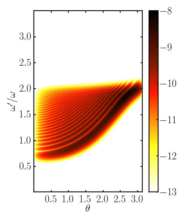
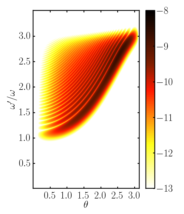
Figure 1: The differential emission probability for the first three harmonics $\ell=1,2$ and $3$ (from left to right panels) in the special reference frame as a function of frequency scaled frequency $\omega^{\prime}/\omega$ and scattering angle $\theta$. The color code denotes the decadic logarithm of $dN_{\ell}/d\omega^{\prime}d\Omega$ in units of inverse eV. The laser has an intensity parameter of $a_{0}=2$ and a pulse length parameter of $\tau=20$.

In general, the interferences between different harmonics are important for differential observables, in particular, for energy resolved spectra, for not too high values of $a_{0}\sim 1$. There, the substructures of the harmonics, which can be seen in Fig. 1, yield interesting spectral information on the non-linear Compton scattering in short laser pulses Seipt and Kämpfer (2010); Mackenroth and Di Piazza (2011). However, for high laser strength, $a_{0}\gg 1$, the differential photon emission probability (31) is a rapidly oscillating function of the photon energy $\omega^{\prime}$. The number of peaks per harmonic is given by $|\Delta f|/\pi\propto|\beta\tau|$ and grows, according to (16), $\propto a_{0}^{2}$. That means, when measuring the energy spectrum with a spectrometer with finite energy resolution, one actually obtains an averaged spectrum. Denoting this average by $\langle\ldots\rangle$, we note that

$$\langle dN\rangle = \sum_{\ell}\langle dN_{\ell}\rangle$$ (33)

which means that the interference terms in (32) average to zero. Also the total photon yield $N$ is determined by the diagonal elements alone, e.g. $\displaystyle N=\sum_{\ell}N_{\ell}$, i.e. the off-diagonal elements give no contribution in the case of $a_{0}\gg 1$. To calculate the photon yield, it is necessary to evaluate the coefficients (21). One could solve this problem by a direct numerical integration. This works very well for not too large values of $a_{0}$ and $\beta$. For higher laser intensity, e.g. already for $a_{0}>20$, $\beta$ can become very large such that the phase exponential is in fact a rapidly oscillating function making a direct numerical integration very difficult.

For rapidly oscillating phase integrals, the stationary phase technique can be applied to the integrals (21) as done e.g. Narozhnyĭ and Fofanv (1996). However, even for large $a_{0}$ there are regions in phase space where the stationary phase method is inapplicable:

1. In the vicinity of the non-linear monochromatic resonance at $s-\ell=\beta$, the stationary points are located at the center of the pulse and very close to each other. There, the the first derivative $g^{\prime}(\phi_{\star})$ is almost zero and, therefore, the stationary phase approximation tends to diverge. The exponent has to be expanded up to the third order derivative Narozhnyĭ and Fofanv (1996) of the phase.

2. The stationary phase approximation is appropriate for large $|\beta|\gg 1$ only. However, in the vicinity of the forward scattering direction $\theta=\pi-\vartheta$ it behaves as $|\beta|=a_{0}^{2}\frac{\omega^{\prime}}{\omega}\frac{\vartheta^{2}}{2}$, thus, the stationary phase method can be applied for angles $\vartheta^{2}\gg a_{0}^{-2}\frac{\omega}{\omega^{\prime}}$ only. Therefore, in the phase space regions where $|\beta|$ is small, a direct numerical evaluation may be used.

Fortunately, these evaluation techniques complement one another, such that they may be combined together by suitable matching conditions $\mathfrak{P}_{1,2}$ (1 and 2 refer to conditions 1.) and 2.) above) to allow for an accurate calculation of the non-linear Compton scattering spectra. The choice of these parameters is motivated in Appendix B. (We note that this method is not restricted to the non-linear Compton scattering process. It can be easily transferred to other strong-field processes such as stimulated pair production Heinzl et al. (2010b) or one-photon annihilation of $e^{+}e^{-}$ pairs Ilderton et al. (2011).)

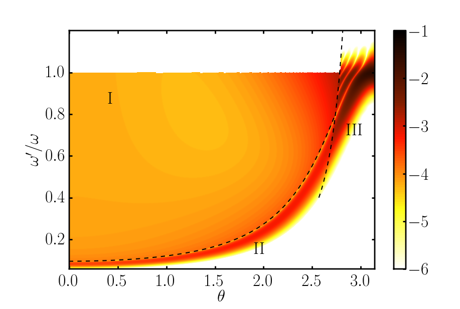
Figure 2: Differential photon yield $dN_{1}/d\omega^{\prime}d\Omega$ as a function of scaled frequency $\omega^{\prime}/\omega$ and scattering angle $\theta$ for $a_{0}=5$, $\tau=25$, and a hyperbolic secant pulse envelope in the special reference frame. In the different areas of phase space (I, II and II, which are delineated by dashed curves), different methods of evaluation for the coefficients $\mathfrak{c}^{m}_{n}$ are employed. Parameters are $\mathfrak{P}_{1}=2.33$ and $\mathfrak{P}_{2}=10$.

We end this section by giving the formula for the phase space averaged photon emission probability which reads

$$\left\langle\frac{d^{2}N_{\ell}}{d\omega^{\prime}d\Omega}\right\rangle = \frac{e^{2}\omega^{\prime}}{64\pi^{3}k\cdot pk\cdot p^{\prime}}\Bigg{\{}(4p\cdot p^{\prime}-8m^{2})(\mathfrak{c}^{0}_{\ell})^{2}-2m^{2}a_{0}^{2}\,\mathfrak{c}^{0}_{\ell}\mathfrak{c}^{2}_{\ell}$$ (34)

$$+\frac{m^{2}a_{0}^{2}}{2}\left(\frac{k\cdot p}{k\cdot p^{\prime}}+\frac{k\cdot p^{\prime}}{k\cdot p}\right)[(\mathfrak{c}^{1}_{\ell+1})^{2}+(\mathfrak{c}^{1}_{\ell-1})^{2}]-2\alpha{k\cdot k^{\prime}}\,\mathfrak{c}^{0}_{\ell}(\mathfrak{c}^{1}_{\ell+1}+\mathfrak{c}^{1}_{\ell-1})\Bigg{\}}$$

with the averaged coefficients $\mathfrak{c}^{m}_{n}$

$$\mathfrak{c}_{\ell-n}^{m} = \left\{\begin{array}[]{lll}J_{\ell-n}(\alpha\sqrt{(s-\ell)/\beta})\sqrt{\frac{s-\ell}{\beta}}^{m}\sqrt{\frac{2\pi}{\Big{|}\beta\sqrt{\frac{s-\ell}{\beta}}g^{\prime}(\phi_{\star})\Big{|}}}&y\geq\mathfrak{P}_{1}\text{ and }|\tau\beta|\geq\mathfrak{P}_{2}&\hat{\equiv}\ {\rm I},\\ \displaystyle 2\pi J_{\ell-n}(\alpha)\frac{1}{|\beta g^{\prime\prime}(0)|^{\frac{1}{3}}}{\rm Ai}(-y)&y<\mathfrak{P}_{1}\text{ and }|\tau\beta|\geq\mathfrak{P}_{2}&\hat{\equiv}\ {\rm II},\\ \displaystyle\int_{-\infty}^{\infty}d\phi J_{\ell-n}(\alpha g)g^{m}(\phi)e^{i(s-\ell)\phi-i\langle\!\langle f\rangle\!\rangle}&|\tau\beta|<\mathfrak{P}_{2}&\hat{\equiv}\ {\rm III}\end{array}\right.$$ (38)

with $y=(s-\ell-\beta)/|\beta g^{\prime\prime}(0)|^{\frac{1}{3}}$. In Appendix B we provide further details on the evaluation of the stationary phase approximation. The regions I, II and III, where the different evaluation schemes for the coefficients apply, are exhibited in Fig. 2. The displayed pattern persists for large values of $a_{0}\gg 1$.

IV Numerical Results

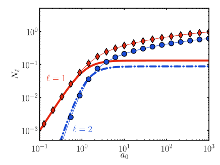
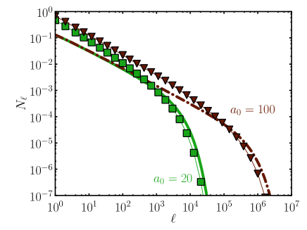
Figure 3: Partial photon yield in hyperbolic secant pulse with $\tau=20$ (symbols) compared to the appropriate yield in a monochromatic wave (thick solid and dashed curves). Matching parameters are $\mathfrak{P}_{1}=2.33$ and $\mathfrak{P}_{2}=20$. Left panel: Behavior of the first two harmonics $N_{1}$ (red diamonds and solid curve) and $N_{2}$ (blue circles and dash-dotted curve) as a function of $a_{0}$. Right panel: Partial emission probabilities $N_{\ell}$ for different laser strength $a_{0}=20$ (green squares and solid curve) and $a_{0}=100$ (brown triangles and dashed curve).

For the numerical evaluation, we consider a laser with frequency (in the laboratory system) of $\omega=1.5\,\rm eV$ colliding head-on with an electron beam with energy of $40\,\rm MeV$. All calculations are performed in the special reference frame. The partial photon yield $N_{\ell}$ for the first and second harmonic per electron in a hyperbolic secant pulse of duration $\tau=20$ are presented in Fig. 3, where it is compared to the appropriate probability expected from a monochromatic pulse. To get a finite number for the photon yield in a monochromatic field comparable with the pulsed laser field we multiply the photon rate $\dot{N}_{\ell}$ in a monochromatic wave with the effective interaction time ${T_{\rm eff}}$ (see eq. (29)), $N_{\ell}={T_{\rm eff}}\dot{N}_{\ell}$, which is a characteristic number for each pulse shape. This corresponds to a normalization to the same energy contained in the laser pulse. Within this approach, both the pulsed and monochromatic photon yields coincide for low $a_{0}\ll 1$, i.e. in the linear interaction regime, the dependence on the pulse shape drops out. For large values of $a_{0}$, the photon yield in a pulsed laser field is enhanced by almost a factor of ten as compared to the photon yield in a monochromatic wave. The differences between pulsed and monochromatic yields at large values of $a_{0}$ express non-linear finite-size effects.

In the right panel of Fig. 3, we display the partial photon yields for fixed $a_{0}=20$ and $100$ as a function of the harmonic number $\ell$ including harmonics up to $\ell=10^{7}$. The cutoff harmonic in a monochromatic laser field can be estimated from the behavior of the Bessel functions at high index and argument and is given by $\ell_{\rm max}\sim a_{0}^{3}$. While for low harmonics the photon yield $N_{\ell}$ is larger in pulsed fields, the ordering of the two curves changes for high harmonics, where the photon yield in a pulsed field pulsed fields is smaller than in a monochromatic wave.

Comparing the total photon yields $N=\sum_{\ell}N_{\ell}$, summed over all harmonics up to $\ell=10^{7}$ in Fig. 4, we find that the total photon yield in a pulsed field exceeds the monochromatic result by a factor of two for $a_{0}=100$. For the monochromatic result we show the sum over the first $140$ harmonics (dashed curve) and an asymptotic approximation (representing the limit $a_{0}\to\infty$) being equivalent to a constant crossed field (solid curve, see e.g. Ritus (1985); Titov et al. (2011)). Additionally, the dotted curve is a rough estimate for the asymptotic probability $N=\alpha_{QED}a_{0}\Delta\phi$ Di Piazza et al. (2010), where we take $\Delta\phi=\omega T_{\rm eff}$ as the relevant phase interval, and $\alpha_{QED}$ is the fine structure constant. For the hyperbolic secant pulse this yields $\Delta\phi=2\tau$.

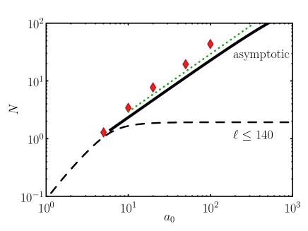
Figure 4: The total photon yield $N$ as a function of $a_{0}$. The result for pulsed laser fields is shown by symbols (red diamonds) being a factor of two above the asymptotic monochromatic result (black solid curve, cf. Titov et al. (2011)). The black dashed curve shows the sum of the first 140 harmonics in a monochromatic wave (compare Titov et al. (2011)). The green dotted curve is a rough approximation to the asymptotic monochromatic result (see the text).

V Summary and Conclusion

In summary, we calculate the photon yield in non-linear Compton scattering at ultra-high intensity $a_{0}\gg 1$ for pulsed laser fields. We use different methods in different parts of phase space, including a stationary phase approximation, where the non-linear phase exponent is very large, and a direct numerical integration in phase space regions where this is not the case. At ultrahigh intensity, an averaging over the substructures in the energy spectrum is included. We find significantly modified partial and total photon yields in pulsed laser fields when comparing to the case of monochromatic laser fields. The partial yield for the first harmonic can be up to a factor of ten larger than the corresponding monochromatic result. For the highest relevant harmonics for a given $a_{0}$ on the order of $\ell\sim a_{0}^{3}$, the photon yield in pulsed fields is typically lower than in monochromatic laser fields. Nonetheless, the summed total probability is by a factor of two larger than the monochromatic result which is typically approximated by a constant crossed field at large values of $a_{0}$. This shows that the constant crossed field approximation is not as good for pulsed laser fields. The method presented here is also be applicable to other processes like stimulated pair production Heinzl et al. (2010b) and one-photon annihilation Ilderton et al. (2011).

Finally, we discuss the relevance of radiation reaction. The radiation reaction is relevant if the parameter $R=\alpha_{QED}\chi a_{0}$ reaches or exceeds unity, where $\chi=a_{0}k\cdot p/m^{2}$ is the quantum nonlinearity parameter. For the parameters used for our numerical calculations and $a_{0}=100$ one finds $R=0.04$, i.e. radiation reaction effects can be neglected. For even higher values of $a_{0}$, however, radiation reaction effects become important. Furthermore, the fact that the quantity related to the emission probability exceeds unity is a hint that multi-photon emission, which is related to radiation reaction Di Piazza et al. (2010), becomes important at these intensities.

Appendix A Beyond the slowly varying envelope approximation

In this section, we go beyond the slowly varying envelope approximation. We give a further justification of the approximation and comment on carrier envelope phase effects. The oscillating part of the non-linear phase exponent has the form

$$\tilde{f}(\phi) = \int d\phi\Big{[}\alpha_{1}g\cos(\phi+\hat{\phi})+\alpha_{2}g\sin(\phi+\hat{\phi})+\beta\cos 2\xi g^{2}\cos 2(\phi+\hat{\phi})\Big{]}$$ (39)

introducing the carrier envelope phase $\hat{\phi}$. This leads to integrals of the form

$$I_{n}=\intop_{-\infty}^{\infty}d\phi\Big{[}g(\phi)e^{i\phi}\Big{]}^{n},\qquad n\in(1,2)$$ (40)

which can be evaluated for a hyperbolic secant pulse with the substitution $x=e^{\phi/\tau}$ as

$$\tilde{f}_{1} = \tau{\rm Re}\left\{\frac{1}{a}(\alpha_{1}-i\alpha_{2})e^{i\hat{\phi}}x^{2a}\,_{2}F_{1}(1,a;a+1;-x^{2})\right\},$$ (41)

$$\tilde{f}_{2} = \beta\tau\cos 2\xi\,{\rm Re}\left\{\frac{1}{a}e^{2i\hat{\phi}}x^{4a}\,_{2}F_{1}(2,2a;2a+1;-x^{2})\right\},$$ (42)

with $\tilde{f}=\tilde{f}_{1}+\tilde{f}_{2}$, $a=(i\tau+1)/2$ and the hypergeometric functions ${}_{2}F_{1}$. For short pulses $\tau\ll 1$, $a\to 1/2$ becomes real. Then, the hypergeometric functions take the limiting values

$${}_{2}F_{1}(1,a;a+1;-x^{2}) \to\ _{2}F_{1}(1,\frac{1}{2};\frac{3}{2};-x^{2})=\arctan x,$$ (43)

$${}_{2}F_{1}(2,2a;2a+1;-x^{2}) \to\ _{2}F_{1}(2,1;2;-x^{2})=\frac{1}{1+x^{2}},$$ (44)

such that

$$\tilde{f}_{1} =2\tau(\alpha_{1}\cos\hat{\phi}+\alpha_{2}\sin\hat{\phi})\arctan\exp{\frac{\phi}{\tau}},$$ (45)

$$\tilde{f}_{2} =\tau\beta\cos 2\xi\,\cos 2\hat{\phi}\,\tanh\frac{\phi}{\tau}.$$ (46)

Thus, the complete phase reads for $\tau\ll 1$

$$f(\phi) =\tau(\alpha_{1}\cos\hat{\phi}+\alpha_{2}\sin\hat{\phi})\arctan\exp{\frac{\phi}{\tau}}+\tau\beta(\cos^{2}\xi\,\cos^{2}\hat{\phi}+\sin^{2}\xi\sin^{2}\hat{\phi})\tanh\frac{\phi}{\tau},$$ (47)

recovering the result of Mackenroth and Di Piazza (2011) for a single-cycle laser pulse with linear polarization, $\xi=0$, and $\hat{\phi}=0$.

In the opposite limit of long pulses, $\tau\gg 1$, $a$ becomes purely imaginary, $a\to i\tau/2$. The slowly varying envelope approximation can be obtained from eqs. (41) and (42) by approximating ${}_{2}F_{1}(n,na;na+1;-x^{2})\to\,_{2}F_{1}(n,na;na;-x^{2})=(x^{2}+1)^{-n}$ yielding eventually Eq. (13). Thus, our general result eqs. (41) and (42) contains both the previous results in the slowly varying envelope approximation for $\tau\gg 1$ and the single-cycle laser pulses for $\tau\ll 1$.

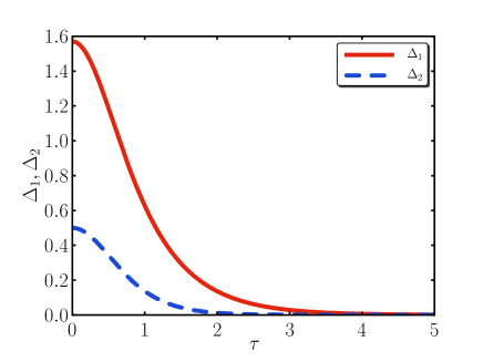
Figure 5: The phase shift functions $\Delta_{1}$ and $\Delta_{2}$ as a function of pulse length $\tau$.

One of the main differences between the slowly varying envelope approximation and the full result is the build-up of an additional phase shift when going from the distant past, $\phi=-\infty$, to distant future, $\phi=+\infty$, in addition to the ponderomotive phase shift $\Delta f=2\beta\tau$. In the slowly varying envelope approximation this phase shift is equal to zero. In the exact expressions for the phase, however, the additional phase shift is non-zero and depends on the carrier envelope phase:

$$\Delta\tilde{f}_{1} = 2\tau\left(\alpha_{1}\cos\hat{\phi}+\alpha_{2}\sin\hat{\phi}\right)\Delta_{1},$$ (48)

$$\Delta\tilde{f}_{2} = 4\tau\beta\cos 2\xi\,\cos 2\hat{\phi}\,\Delta_{2},$$ (49)

$$\Delta_{1} = \frac{1}{2}{\rm Re}\left\{\psi(\frac{a+1}{2})-\psi(\frac{a}{2})\right\},$$ (50)

$$\Delta_{2} = \frac{1}{2}{\rm Re}\left\{1+(1-2a)[\psi(\frac{2a+1}{2})-\psi(a)]\right\},$$ (51)

where $\psi(z)=\frac{d}{dz}\log\Gamma(z)$ is the digamma function. Thus, the total phase shift becomes now $\Delta f=2\beta\tau+\Delta\tilde{f}_{1}+\Delta\tilde{f}_{2}$, where the first term is the ponderomotive phase shift originating from $\langle\!\langle f\rangle\!\rangle$.

The functions $\Delta_{1}$ and $\Delta_{2}$, depending only on the pulse length $\tau$, are depicted in Fig. 5. The additional phase is relevant for $\tau<5$ only. For longer pulsed the phase shifts drop to zero exponentially fast. This explains why the slowly varying envelope is much better than expected; even down to $\tau=5$ although it appears as an expansion in inverse powers of $\tau$. It should be clear that this additional phase shift modifies the positions of the stationary phase points and, therefore, also the support and number and position of zeros of the coefficient functions $c^{m}_{\ell-n}$.

Appendix B Stationary phase, zero convexity approximations and matching conditions

B.1 Stationary phase approximation

The stationary phase approximation of (21) at a certain value of $s$ is given by the sum of the contributions from the two stationary points

$$c_{\ell-n}^{m}(s-\ell) = J_{\ell-n}\big{(}\alpha g(\phi_{\star})\big{)}g^{m}(\phi_{\star})\sqrt{\frac{2\pi}{|\beta G_{2}^{\prime\prime}(\phi_{\star})|}}\exp\left\{i(s-\ell)\phi_{\star}-i\beta G_{2}(\phi_{\star})-i\frac{\pi}{4}\right\}$$ (52)

$$+J_{\ell-n}\big{(}\alpha g(-\phi_{\star})\big{)}g^{m}(-\phi_{\star})\sqrt{\frac{2\pi}{|\beta G_{2}^{\prime\prime}(-\phi_{\star})|}}\exp\left\{-i(s-\ell)\phi_{\star}-i\beta G_{2}(-\phi_{\star})+i\frac{\pi}{4}\right\}$$

$$= 2J_{\ell-n}\big{(}\alpha g(\phi_{\star})\big{)}g^{m}(\phi_{\star})\sqrt{\frac{2\pi}{|\beta G_{2}^{\prime\prime}(\phi_{\star})|}}\cos\left\{(s-\ell)\phi_{\star}-\beta G_{2}(\phi_{\star})-\frac{\pi}{4}\right\}.$$

The oscillations of the coefficient functions $c^{m}_{\ell-n}$ stem from the cosine term which is a common factor in all contributions to the partial matrix element $\mathrsfs M_{\ell}$. When squaring the matrix element to calculate the partial differential photon emission probability $dN_{\ell}$, we obtain a $\cos^{2}$ behavior, which averages to $1/2$. Because the interferences cancel on average, we may replace the cosine in (52) by $1/\sqrt{2}$ and write for the averaged function

$$\langle c_{\ell-n}^{m}(s-\ell)\rangle = J_{\ell-n}\big{(}\alpha g(\phi_{\star})\big{)}g^{m}(\phi_{\star})\sqrt{\frac{4\pi}{|\beta G_{2}^{\prime\prime}|}}.$$ (53)

We now estimate the number of zeros of $c^{m}_{n-\ell}$ which is also the number of subpeaks in a given harmonic. The functions $c^{m}_{n-\ell}$ are zero when the contributions from the two symmetric stationary points interfere destructively; i.e. whenever the phase fulfills the equation

$$\beta\left[\phi_{k}g^{2}(\phi_{k})-\int_{0}^{\phi_{k}}d\phi g^{2}(\phi)\right]-\left(\frac{1}{4}-k\right)\pi=0$$ (54)

defining a series $(s_{k})_{k=1\ldots K}$ of zeros of $c_{\ell-n}^{m}(s-\ell)$. The number $K$ of zeros is determined by the range of values the term in the square brackets can take restricting the largest and smallest allowed values of $k$. Noting that the function in the square brackets in (54) is a monochromatic dropping function of its argument it suffices to consider its values at $\pm\infty$. However, the first term goes to zero when approaching infinity and the second term (including the leading $\beta$ term) is $\langle\!\langle f\rangle\!\rangle$ . Thus, $\pi(k_{\rm max}-k_{\rm min})\sim|\langle\!\langle f\rangle\!\rangle(\infty)-\langle\!\langle f\rangle\!\rangle(-\infty)|$ and the number of zeros $K$ is determined by the total ponderomotive phase shift $\displaystyle\Delta f$ as $K\sim|\Delta f|/\pi\propto|\beta\tau|/\pi$. This result is a generalization of the findings of Hartemann et al. (2010) within the classical theory of Thomson scattering for hyperbolic cosine pulse shapes in the backscattering direction to the quantum theory of Compton scattering for arbitrary pulse shapes and arbitrary scattering angles.

B.2 Zero convexity approximation

In the vicinity of $\phi=0$ the stationary phase approximation diverges. One must expand the exponent up to the third derivative, around the point of zero convexity (i.e. the second derivative of the phase in (21) vanishes) yielding the approximation

$$c_{\ell-n}^{m}(s-\ell) \cong 2\pi J_{\ell-n}(\alpha)\left(\frac{1}{|\beta g^{\prime\prime}(0)|}\right)^{\frac{1}{3}}{\rm Ai}(-y),$$ (55)

$$y = \frac{s-\ell-\beta}{|\beta g^{\prime\prime}(0)|^{\frac{1}{3}}},$$ (56)

where ${\rm Ai}(y)=\frac{1}{2\pi}\int_{-\infty}^{\infty}dt\exp\{iyt+it^{3}/3\}$ is the Airy function.

The height and shape of the main peak of the spectrum are determined by the curvature of $g(\phi)$ at the center of the pulse, where the second derivative vanishes. The main peak is the same for hyperbolic secant and Gaussian envelopes, because the second derivative at the origin is the same. The only difference comes from the different behavior of the first derivative in the stationary phase approximation. This determines the different shape of the spectra in the high-energy tail of each harmonic.

B.3 Matching Conditions

Here we motivate our choices for the matching parameters $\mathfrak{P}_{1,2}$. The parameter $\mathfrak{P}_{1}$ determines the transition between the stationary phase approximation and the zero convexivity approximation. We define the matching point by $y=\mathfrak{P}_{1}$ which should be in the range $1.4<\mathfrak{P}_{1}<2.3381$ because for smaller $\mathfrak{P}_{1}$ the two stationary phase points would be too close to each other Narozhnyĭ and Fofanv (1996) and for larger values the two approximations start to differ too much. We use the stationary phase approximation for $y\geq\mathfrak{P}_{1}$ (region I in Fig. 2) and zero convexity approximation for $y<\mathfrak{P}_{1}$ (region II in Fig. 2).

The parameter $\mathfrak{P}_{2}$ determines the matching between the direct numerical evaluation and the stationary phase/zero convexity approximation. The approximations for the functions $c^{m}_{\ell-n}$ are used whenever $|\tau\beta|>\mathfrak{P}_{2}$ and the full numerical results otherwise (region II in Fig. 2). The numerical result was found to be rather insensitive to the explicit value in the range $10<\mathfrak{P}_{2}<50$.

References

- Yanovsky et al. (2008) V. Yanovsky et al., Opt. Express 16, 2109 (2008).
- (2) http://extreme-light-infrastructure.eu.
- Salamin et al. (2006) Y. I. Salamin, S. X. Hu, K. Z. Hatsagortsyan, and C. H. Keitel, Phys. Reports 427, 41 (2006).
- Fedotov et al. (2010) A. M. Fedotov, N. B. Narozhny, G. Mourou, and G. Korn, Phys. Rev. Lett. 105, 080402 (2010).
- Bell and Kirk (2008) A. R. Bell and J. G. Kirk, Phys. Rev. Lett. 101, 200403 (2008).
- Krafft (2004) G. A. Krafft, Phys. Rev. Lett. 92, 204802 (2004).
- Gao (2004) J. Gao, Phys. Rev. Lett. 93, 243001 (2004).
- Hartemann et al. (1996) F. V. Hartemann, A. L. Troha, N. C. Luhmann, and Z. Toffano, Phys. Rev. E 54, 2956 (1996).
- Heinzl et al. (2010a) T. Heinzl, D. Seipt, and B. Kämpfer, Phys. Rev. A 81, 022125 (2010a).
- Narozhnyĭ and Fofanv (1996) N. B. Narozhnyĭ and M. S. Fofanv, JETP 83, 14 (1996).
- Boca and Florescu (2009) M. Boca and V. Florescu, Phys. Rev. A 80, 053403 (2009).
- Seipt and Kämpfer (2010) D. Seipt and B. Kämpfer, Phys. Rev. A 83, 022101 (2010).
- Mackenroth and Di Piazza (2011) F. Mackenroth and A. Di Piazza, Phys. Rev. A 83, 032106 (2011).
- Seipt and Kämpfer (2011) D. Seipt and B. Kämpfer, Phys. Rev. ST AB 14, 040704 (2011).
- Volkov (1935) D. M. Volkov, Z. Phys. 94, 250 (1935).
- Ilderton (2011) A. Ilderton, Phys. Rev. Lett. 106, 020404 (2011).
- Korsch et al. (2006) H. J. Korsch, A. Klumpp, and D. Witthaut, J. Phys. A 39, 14947 (2006).
- Berestetzki et al. (1980) W. B. Berestetzki, E. M. Lifschitz, and L. P. Pitajewski, Relativistische Qantentheorie, Lehrbuch der Theoretischen Physik, Vol. IV (Akademie Verlag Berlin, 1980).
- Heinzl et al. (2010b) T. Heinzl, A. Ilderton, and M. Marklund, Phys. Lett. B 692, 250 (2010b).
- Ilderton et al. (2011) A. Ilderton, P. Johansson, and M. Marklund, Phys. Rev. A 84, 032119 (2011).
- Ritus (1985) V. I. Ritus, J. Sov. Laser Res. 6, 497 (1985).
- Titov et al. (2011) A. I. Titov, B. Kämpfer, H. Takabe, and A. Hosaka, Phys. Rev. D 83, 053008 (2011).
- Di Piazza et al. (2010) A. Di Piazza, K. Z. Hatsagortsyan, and C. H. Keitel, Phys. Rev. Lett. 105, 220403 (2010).
- Hartemann et al. (2010) F. V. Hartemann, F. Albert, C. W. Siders, and C. P. J. Barty, Phys. Rev. Lett. 105, 130801 (2010).