Rapidly rotating plane layer convection with zonal flow

Abstract

The onset of convection in a rapidly rotating layer in which a thermal wind is present is studied. Diffusive effects are included. The main motivation is from convection in planetary interiors, where thermal winds are expected due to temperature variations on the core-mantle boundary. The system admits both convective instability and baroclinic instability. We find a smooth transition between the two types of modes, and investigate where the transition region between the two types of instability occurs in parameter space. The thermal wind helps to destabilise the convective modes. Baroclinic instability can occur when the applied vertical temperature gradient is stable, and the critical Rayleigh number is then negative. Long wavelength modes are the first to become unstable. Asymptotic analysis is possible for the transition region and also for long wavelength instabilities, and the results agree well with our numerical solutions. We also investigate how the instabilities in this system relate to the classical baroclinic instability in the Eady problem. We conclude by noting that baroclinic instabilities in the Earth’s core arising from heterogeneity in the lower mantle could possibly drive a dynamo even if the Earth’s core were stably stratified and so not convecting.

1 Introduction

The geomagnetic field is believed to be generated by convection in the Earth’s fluid outer core. The convection in the core is strongly influenced by rotation, leading to the formation of tall thin columns which transport the heat out from the interior to the core-mantle boundary (Busse and Carrigan, 1976; Jones, 2000). The form of these columns plays a vital role in the mechanism by which magnetic field is generated (Olson et al., 1999). Although the convection in the core is in a strongly nonlinear regime, with Rayleigh number well above that at the onset of convection, dynamo models show that the convecting columns still have many features that resemble the pattern of convection derived from linear theory.

The onset of convection from stationary fluid in rapidly rotating spherical bodies is now fairly well understood. Roberts (1968) and Busse (1970) evaluated the essential principles, confirmed in numerical studies by Zhang (1992). The behaviour in the asymptotic limit of small Ekman number (rapid rotation) was elucidated by Jones et al. (2000) and Dormy et al. (2004). In this paper we study the onset of convection in a rotating system with an imposed zonal flow, that is an axisymmetric, azimuthal flow. Zonal flows occur frequently in nature. Well-known examples are the wind systems on the giant planets, where east-west flows reaching up to several hundreds of metres per second can occur. The systems most relevant to this paper are the cases where the zonal flow is a thermal wind, driven by latitudinal temperature gradients. A famous example is the jet-stream in our atmosphere, driven by the pole-equator temperature difference. Thermal winds are also believed to occur in the Earth’s core (Olson and Aurnou, 1999; Sreenivasan and Jones, 2005, 2006) where warmer regions above the poles lead to anticyclonic vortices which can be detected in the secular variation as the geomagnetic field is advected by the flow. This process has been modelled in the laboratory by Aurnou et al. (2003).

Convection in the outer core is significantly affected by the presence of a solid inner core of radius approximately 0.35 times the radius of the fluid outer core. The fundamental cause of the warmer (and compositionally lighter) regions near the poles is believed to be the different efficiency of convection in the polar regions inside the tangent cylinder and outside the tangent cylinder (Tilgner and Busse, 1997). The tangent cylinder is the imaginary cylinder that touches the inner core; outside the tangent cylinder convection columns can reach right across the outer core, but inside the tangent cylinder columns are bounded by the inner core. Thermal winds inside the Earth’s core could also arise more directly, because of a heterogeneous heat flux across the core-mantle boundary. Seismic tomography suggests that heterogeneities exist, and a natural interpretation is that the variations in seismic velocity are due to thermal variations caused by a core-mantle heat flux that varies with latitude and longitude (Gubbins et al., 2007). In this situation, even when the temperature gradient is subadiabatic so convection would not be expected, a basic state with no flow is impossible (see e.g. Zhang and Gubbins, 1996). A thermal wind is set up which might lead to a baroclinic instability. The possibility that the core is stably stratified just below the core-mantle boundary was originally suggested by Braginsky (1993). While we do not currently know whether the core heat flux is low enough for such a subadiabatic region to exist, estimates of the thermal conditions in the core suggest it is a realistic possibility (Anufriev et al., 2005).

The aim of this paper is to examine the effect of a thermal wind on the onset of convection, and to examine whether baroclinic instabilities can arise in rapidly rotating systems when the fluid is stably stratified. As we see below, as the thermal wind is gradually increased, convective modes evolve into baroclinic modes. The critical Rayleigh number can therefore become negative when the thermal wind flow is large enough that baroclinicity becomes important. This can occur at conditions which are realistic for the core. To elucidate the fundamental mechanisms involved, we consider here a simple plane layer model, which allows some asymptotic limits to be explored. This simple model is most relevant to the polar regions in the core, since we are taking gravity and rotation to be parallel. More realistic geometries for core convection will be explored subsequently.

The onset of rotating convection in a plane layer in the absence of a thermal wind was comprehensively studied by Chandrasekhar (1961). Baroclinic instability in a stably stratified layer forms the basis of the Eady problem, discussed in detail in the meteorological context by Pedlosky (1987) and Drazin and Reid (1981). Here we combine these two classical problems by examining the stability of a simple thermal wind state when diffusion is present and when the vertical temperature gradient, specified by the Rayleigh number, can be either positive or negative.

2 Description of the model

We consider a plane layer of depth $d$ rotating about the vertical axis with angular velocity $\Omega$. We choose a Cartesian coordinate system with the origin situated at the centre of the layer so that the boundaries are located at $z=\pm d/2$. In this geometry $x$ and $y$ are playing the role of the azimuthal and latitudinal coordinates respectively. The static temperature gradient in the absence of the zonal flow is such that $T=\beta d$ and $T=0$ at $z=-d/2$ and $z=d/2$ respectively. Gravity, $g$, acts downwards in the negative $z$-direction. This type of setup is appropriate for polar regions of the Earth’s core where gravity is near parallel to the rotation axis and the zonal flows are expected to depend on $z$.

The equation of motion in a rotating frame whilst assuming the Boussinesq approximation is

$$\frac{\partial\mathbf{U}}{\partial t}+(\mathbf{U}\cdot\nabla)\mathbf{U}+2\Omega\mathbf{\hat{z}}\times\mathbf{U} = -\frac{1}{\rho_{0}}\nabla\mathcal{P}+g\alpha T\mathbf{\hat{z}}+\nu\nabla^{2}\mathbf{U},$$ (1)

and the temperature equation is

$$\frac{\partial T}{\partial t}+(\mathbf{U}\cdot\nabla)T = \kappa\nabla^{2}T,$$ (2)

where $\alpha$, $\nu$ and $\kappa$ are the coefficient of thermal expansion, the kinematic viscosity and the thermal diffusivity respectively, $\mathcal{P}$ being the pressure and $\rho_{0}$ the density. Also, the Boussinesq continuity equation is simply

$$\nabla\cdot\mathbf{U}=0.$$ (3)

2.1 Basic state

In many models the basic state has a velocity field set to zero and we have hydrostatic balance in the momentum equation between the pressure gradient and the buoyancy. When this is the case taking the curl of (1) results in a $T$ that can only vary in the direction parallel to gravity. However if the basic state temperature varies in the $x$ or $y$ direction we must have a balance between the pressure gradient, buoyancy and Coriolis force in the momentum equation. By taking the curl of (1) in this case we obtain the thermal wind equation

$$2\Omega\frac{\partial\mathbf{U}}{\partial z}=g\alpha\mathbf{\hat{z}}\times\nabla T,$$ (4)

which generates an azimuthal zonal flow, the thermal wind, when $T$ has $y$-dependence.

Since we want a thermal wind in our basic state, we set $\mathbf{U}$, $T$ and $\mathcal{P}$ as $\mathbf{u_{0}}$, $T_{0}$ and $p_{0}$ respectively, and let

$$\mathbf{u_{0}} = u^{\prime}z\mathbf{\hat{x}},$$ (5)

$$T_{0} = \beta\left(\frac{d}{2}-z\right)-\frac{2\Omega u^{\prime}}{g\alpha}y,$$ (6)

$$p_{0} = g\alpha\beta\rho_{0}\left(\frac{zd}{2}-\frac{z^{2}}{2}\right)-2\rho_{0}\Omega u^{\prime}yz+p_{\textrm{constant}},$$ (7)

which is a solution to the system of equations (1) - (4), where $\beta$ is the static temperature gradient in the absence of the zonal flow. Here $u^{\prime}$ is the constant shear defining the strength of the zonal flow. These equations define the basic state. Of particular note here is the fact that the temperature distribution depends on a coordinate other than the coordinate parallel to the rotation axis, so the basic state is baroclinic, that is $\nabla p_{0}$ is not parallel to $\nabla\rho=-\alpha\rho_{0}\nabla T_{0}$.

2.2 Perturbed state

In order to analyse linear stability we now add small perturbations to the basic state so that $\mathbf{U}=\mathbf{u_{0}}+\mathbf{u}$, $\mathcal{P}=p_{0}+p$ and $T=T_{0}+\theta$. Since the perturbations are small we are able to ignore nonlinear terms so that equations (1) and (2), using the definition of the basic state, give

$$\frac{\partial\mathbf{u}}{\partial t}+u^{\prime}z\frac{\partial\mathbf{u}}{\partial x}+u^{\prime}u_{z}\mathbf{\hat{x}}+2\Omega\mathbf{\hat{z}}\times\mathbf{u}=-\frac{1}{\rho_{0}}\nabla p+g\alpha\theta\mathbf{\hat{z}}+\nu\nabla^{2}\mathbf{u},$$ (8)

$$\frac{\partial\theta}{\partial t}+u^{\prime}z\frac{\partial\theta}{\partial x}-\beta u_{z}-\frac{2\Omega u^{\prime}}{g\alpha}u_{y}=\kappa\nabla^{2}\theta.$$ (9)

We proceed by eliminating the pressure to leave four equations for four unknowns. We denote the vorticity by $\omega$ and then the $z$-components of the curl and double curl of equation (8) are

$$\frac{\partial\omega_{z}}{\partial t}+u^{\prime}z\frac{\partial\omega_{z}}{\partial x}-u^{\prime}\frac{\partial u_{z}}{\partial y}-2\Omega\frac{\partial u_{z}}{\partial z}=\nu\nabla^{2}\omega_{z},$$ (10)

$$\frac{\partial\nabla^{2}u_{z}}{\partial t}+u^{\prime}z\frac{\partial\nabla^{2}u_{z}}{\partial x}+2\Omega\frac{\partial\omega_{z}}{\partial z}=g\alpha\nabla_{H}^{2}\theta+\nu\nabla^{4}u_{z},$$ (11)

respectively. Here $\nabla_{H}^{2}=\partial^{2}/\partial x^{2}+\partial^{2}/\partial y^{2}$ is the horizontal Laplacian. Then by employing the identity $\partial\omega_{z}/\partial x-\partial^{2}u_{z}/\partial y\partial z=\nabla_{H}^{2}u_{y}$, equation (9) can be written

$$\nabla_{H}^{2}\left(\frac{\partial\theta}{\partial t}+u^{\prime}z\frac{\partial\theta}{\partial x}-\beta u_{z}-\kappa\nabla^{2}\theta\right)=\frac{2\Omega u^{\prime}}{g\alpha}\left(\frac{\partial\omega_{z}}{\partial x}-\frac{\partial^{2}u_{z}}{\partial y\partial z}\right).$$ (12)

We now have three equations (10) - (12) for three unknowns, namely: $u_{z}$, $\omega_{z}$ and $\theta$. Next we non-dimensionalise these equations using length scale $d$, time scale $d^{2}/\nu$ and temperature scale $\beta\nu d/\kappa$. Then equations (10) - (12) become

$$\left(\frac{\partial}{\partial t}+Rez\frac{\partial}{\partial x}-\nabla^{2}\right)\omega_{z}-Re\frac{\partial u_{z}}{\partial y}-E^{-1}\frac{\partial u_{z}}{\partial z}=0,$$ (13)

$$\left(\frac{\partial}{\partial t}+Rez\frac{\partial}{\partial x}-\nabla^{2}\right)\nabla^{2}u_{z}+E^{-1}\frac{\partial\omega_{z}}{\partial z}=Ra\nabla_{H}^{2}\theta,$$ (14)

$$P\left(\frac{\partial}{\partial t}+Rez\frac{\partial}{\partial x}-P^{-1}\nabla^{2}\right)\nabla_{H}^{2}\theta=\nabla_{H}^{2}u_{z}+\frac{PRe}{ERa}\left(\frac{\partial\omega_{z}}{\partial x}-\frac{\partial^{2}u_{z}}{\partial y\partial z}\right),$$ (15)

where the Ekman number, $E$, Prandtl number, $P$, Rayleigh number, $Ra$, and Reynolds number, $Re$, are defined as

$$E=\frac{\nu}{2\Omega d^{2}},\qquad P=\frac{\nu}{\kappa},\qquad Ra=\frac{g\alpha\beta d^{4}}{\nu\kappa},\qquad Re=\frac{u^{\prime}d^{2}}{\nu}.$$ (16)

Equations (13) - (15) are the finite Ekman number equations for rapidly rotating plane layer convection with zonal flow. Our system is defined so that when $\beta>0$ we have cold fluid sitting on top of hot fluid and thus the layer is buoyantly unstable. Therefore, as is usually the case when considering thermal convection, we require a positive Rayleigh number above some critical value, $Ra_{c}$, for convective motions to begin. In the case where $\beta<0$ the system is buoyantly stable since hot fluid sits on top of cold fluid and with a basic state temperature distribution only dependent on $z$ no convection is possible. However, since the basic state temperature distribution we have defined in section 2.1 depends on $y$ as well as $z$ it is not immediately clear if motion is forbidden when $Ra<0$ in our setup.

3 Numerics

The solutions were assumed to take the form: $\exp(\sigma t+\mathrm{i}(k_{x}x+k_{y}y))$ where the growth rate, $\sigma$, is in general, complex. The resulting equations are

$$\left(\sigma+\mathrm{i}k_{x}Rez+k^{2}-\frac{\mathrm{d}^{2}}{\mathrm{d}z^{2}}\right)\omega_{z}-\mathrm{i}k_{y}Reu_{z}-E^{-1}\frac{\mathrm{d}u_{z}}{\mathrm{d}z}=0,$$ (17)

$$\left(\sigma+\mathrm{i}k_{x}Rez+k^{2}-\frac{\mathrm{d}^{2}}{\mathrm{d}z^{2}}\right)\left(\frac{\mathrm{d}^{2}}{\mathrm{d}z^{2}}-k^{2}\right)u_{z}+E^{-1}\frac{\mathrm{d}\omega_{z}}{\mathrm{d}z}=-k^{2}Ra\theta,$$ (18)

$$\left(\sigma P+\mathrm{i}k_{x}PRez+k^{2}-\frac{\mathrm{d}^{2}}{\mathrm{d}z^{2}}\right)\theta=u_{z}-\frac{\mathrm{i}PRe}{ERak^{2}}\left(k_{x}\omega_{z}-k_{y}\frac{\mathrm{d}u_{z}}{\mathrm{d}z}\right),$$ (19)

where $k^{2}=k_{x}^{2}+k_{y}^{2}$. In addition to demanding that there be no penetration ($u_{z}$=0) and a constant surface temperature ($\theta$=0) at the boundaries, we considered two cases, namely stress-free and no-slip boundary conditions on both the upper and lower boundaries so that

$$\frac{\mathrm{d}^{2}u_{z}}{\mathrm{d}z^{2}}= 0=\frac{\mathrm{d}\omega_{z}}{\mathrm{d}z}\ \textrm{at}\ z=\pm\frac{1}{2}\ \textrm{for the stress-free case,}$$ (20)

$$\frac{\mathrm{d}u_{z}}{\mathrm{d}z}= 0=\omega_{z}\ \textrm{at}\ z=\pm\frac{1}{2}\ \textrm{for the no-slip case.}$$ (21)

We solved equations (17) - (19) using a simple eigenvalue solver. The system has the following six input parameters: $k_{x}$, $k_{y}$, $Re$, $P$, $E$ and $Ra$, which can be varied to obtain the growth rate. Given values for the other five parameters we are interested in finding the Rayleigh number, $Ra^{*}$, at the onset of convection. Hence for various values of the input parameters we searched for marginal modes, where $\Re[\sigma]=0$, and recorded the value of $Ra^{*}$ for which the mode appeared. To reduce the parameter space we worked with typical values of the Ekman number $(E\sim 10^{-3}-10^{-5})$ and Prandtl number $(P\sim 0.1-10)$.

Figure 1 shows how the onset of convection changes as the azimuthal wavenumber and the zonal wind are varied for a particular choice of the Ekman number, Prandtl number and the latitudinal wavenumber, for both choices of boundary conditions. It should be noted that the data in figure 1 is represented on a log-log plot due to the varying magnitudes involved, and a log scale is necessary for the values of $Ra^{*}$ also. Since we have positive and negative Rayleigh numbers, we plot only contours with $|Ra^{*}|>1$, but this excludes only a tiny region in figures 1(a) and 1(b). Also of note is the fact that the quantity which has been plotted, $Ra^{*}$, is not the same as the critical Rayleigh number, $Ra_{c}$, since the latter is minimised over the wavenumbers, $k_{x}$ and $k_{y}$. We plot $Ra^{*}$ here rather than the critical Rayleigh number due to reasons discussed in section 3.2. Plots for $Ra_{c}$ are displayed later. The initial striking feature of both sets of results is the appearance of marginal modes with negative Rayleigh number. We see that these modes only appear under certain parameter regimes, namely for sufficiently large $Re$ and sufficiently small $k_{x}$. Hence we are able to divide the parameter space into two regimes driven by different types of instability: the convective regime and the baroclinic regime. In the convective/baroclinic regime it is the buoyancy/shear, which is driving the instability. The form of the eigenfunctions in $xz$-space for the points marked in figure 1 is shown in figure 2.

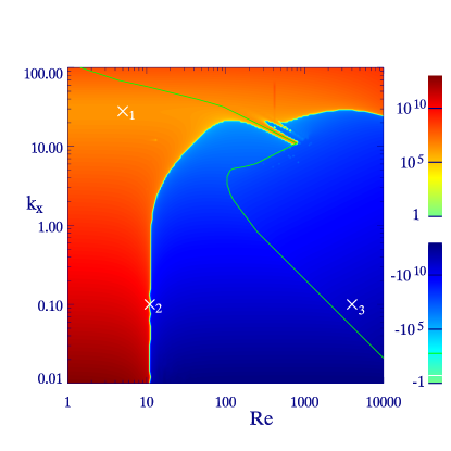
(a) Stress-free boundaries.

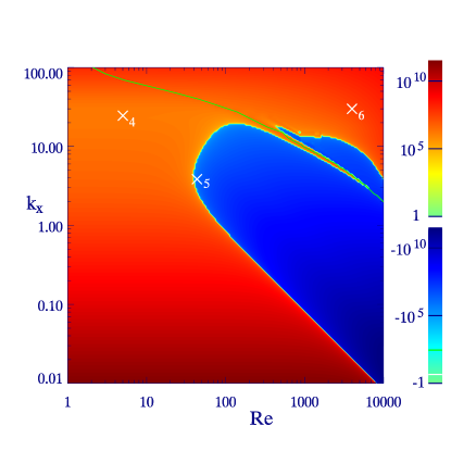
(b) No-slip boundaries.

Figure 1: Contour plots of the numerical results for the Rayleigh number at onset for $Re$ against $k_{x}$ with $E=10^{-4}$, $P=1$, $k_{y}=k_{y_{c}}=0$. The colour scales denote the value of the Rayleigh number at onset, $Ra^{*}$. The green curves divide the regions of steady modes and oscillatory modes, onset being oscillatory to the right of these curves.

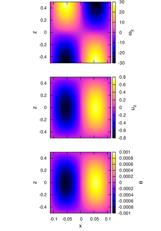
(a) $\times_{1}$

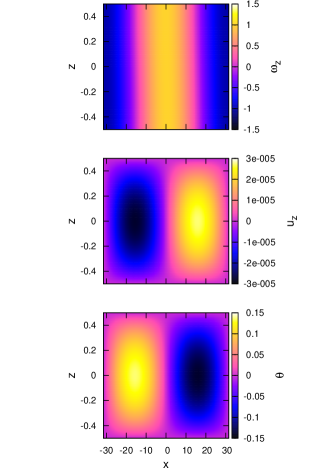
(b) $\times_{2}$

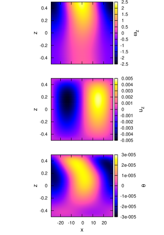
(c) $\times_{3}$

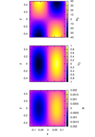
(d) $\times_{4}$

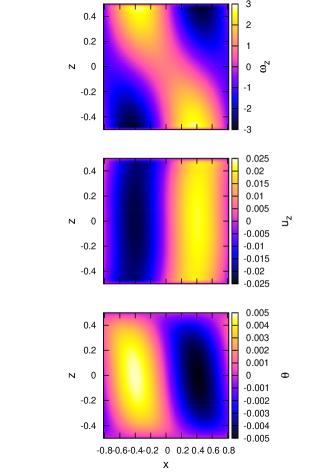
(e) $\times_{5}$

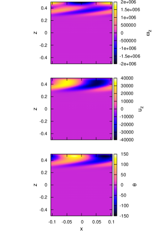
(f) $\times_{6}$

Figure 2: Eigenfunction plots corresponding to points marked on figure 1. Stress-free cases: $\times_{1}:Re=5,\ Ra=Ra_{c}\equiv 1.8889\times 10^{6},\ k_{x}=k_{x_{c}}\equiv 27.9610.\ \times_{2}:Re=Re^{*}\equiv 10.9599,\ Ra=-10^{6},\ k_{x}=0.1.\ \times_{3}:Re=4000,\ Ra=Ra^{*}\equiv-1.3571\times 10^{11},\ k_{x}=0.1.\$ No-slip cases: $\times_{4}:Re=5,\ Ra=Ra_{c}\equiv 1.5193\times 10^{6},\ k_{x}=k_{x_{c}}\equiv 24.5630.\ \times_{5}:Re=Re_{c}\equiv 43.4458,\ Ra=-10^{6},\ k_{x}=k_{x_{c}}\equiv 3.8551.\ \times_{6}:Re=4000,\ Ra=Ra^{*}\equiv 3.1259\times 10^{7},\ k_{x}=30.$ $k_{y}=k_{y_{c}}=0$ for all points.

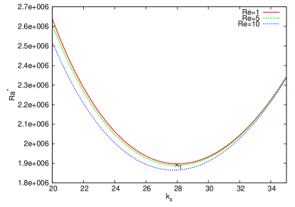
(a) Stress-free boundaries.

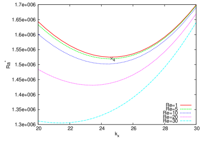
(b) No-slip boundaries.

Figure 3: Plots of the numerical results for the onset parameters in the convective regime against $k_{x}$ with $E=10^{-4}$, $P=1$, $k_{y}=k_{y_{c}}=0$. The onset parameter is the Rayleigh number in the convective regime.

3.1 Convective regime

For low values of the zonal wind we expect to find the usual convective columnar roll solutions as described by Chandrasekhar (1961), which we refer to as the ‘convective modes’. Convective modes with the $z$-vorticity antisymmetric about the equator are expected as the most unstable modes in plane layer convection; the converse is true in the case of the full sphere as originally noted by Busse (1970). Indeed for the point marked $\times_{1}$ we find the mode to be of this form, as shown by figure 2(a). The structure has tall thin cells with hot fluid rising and cold fluid sinking as expected. This is the case for both types of boundary conditions as is evident from the similarity of figure 2(d), point $\times_{4}$, for the no-slip case. We also note that for $Re=0$ if we minimise the Rayleigh number at onset over $k$, to find the critical Rayleigh number, the preferred values are $Ra_{c}\sim 1.8970\times 10^{6}$ with $k_{c}\sim 28.0243$ for the stress-free case and $Ra_{c}\sim 1.5251\times 10^{6}$ with $k_{c}\sim 24.6366$ for the no-slip case, for the values of $E$ and $P$ used in figure 1. This is in agreement with Chandrasekhar (1961). These critical values of the wavenumbers do however depend on $Re$. In the case of $Re=0$ the system has complete symmetry in the $x$ and $y$ directions, so all wavenumbers $k_{x}$ and $k_{y}$ satisfying $k_{x}^{2}+k_{y}^{2}=k_{c}^{2}$ onset at $Ra_{c}$. However as the zonal wind strength is increased from zero we found there is immediately a preference for two-dimensional modes with $k_{y_{c}}=0$. This is the case for all modes with $Re\neq 0$. We also find that the value of the critical Rayleigh number decreases, for both types of boundary conditions, as shown by figure 3. Hence the zonal wind has a destabilising effect on the system and aids the onset of convection. The critical azimuthal wavenumber, $k_{x_{c}}$, also decreases as $Re$ is increased for both types of boundary conditions as shown by figure 3. The two plots of eigenfunctions in the convective regime, $\times_{1}$ and $\times_{4}$ are for critical values of $k_{x}$ and $Ra^{*}$ with $Re=5$.

As $Re$ is increased we move into the baroclinic regime and hence the values of $Re$ chosen for the plot in figure 3 are relatively low in order to remain in the convective regime. For the modes in the convective regime the main energy balance is between the buoyancy and the viscous stresses. However as $Re$ is increased, the baroclinic basic state means that buoyancy can do work at lower critical Rayleigh number, and indeed even at negative Rayleigh number. This is discussed in section 3.4.

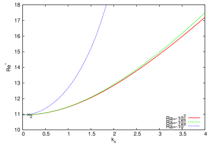
(a) Stress-free boundaries.

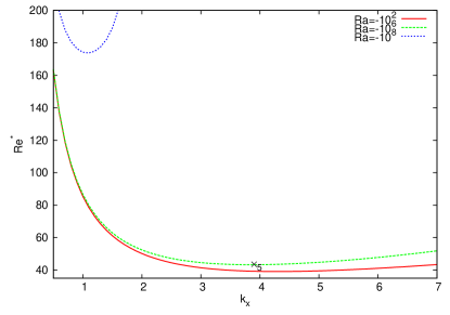
(b) No-slip boundaries.

Figure 4: Plots of the numerical results for the onset parameters in the baroclinic regime against $k_{x}$ with $E=10^{-4}$, $P=1$, $k_{y}=k_{y_{c}}=0$. The onset parameter is the Reynolds number in the baroclinic regime.

3.2 Baroclinic regime

As the zonal wind strength is increased further we find a second type of mode, which is interesting as it allows for instability regardless of how negative the Rayleigh number is. In other words this mode can be unstable no matter how stably stratified the system is. For this reason we refer to them as ‘baroclinic modes’, which are distinct from the convective modes that are usually found as the most unstable modes. They are related to the unstable modes of the Eady problem (Pedlosky, 1987). This suggests that we should consider a critical Reynolds number, rather than a critical Rayleigh number, for the baroclinic modes since it is the shear that is driving this instability. Hence we introduce a critical Reynolds number, $Re_{c}$, and corresponding critical wavenumbers, $k_{x_{c}}$ and $k_{y_{c}}$ for the baroclinic regime. For a given Ekman number, Prandtl number and Rayleigh number $Re_{c}$ is the value of the Reynolds number for which a marginal baroclinic mode can appear (analogous to the critical Rayleigh number in the convective regime). As with all modes with a non-zero Reynolds number we find that $k_{y_{c}}=0$. From figure 4 we see how $Re^{*}$ varies with $k_{x}$ for several negative values of the Rayleigh number for both types of boundary conditions.

For stress-free boundaries we see from figure 4(a) that in all cases $k_{x_{c}}=0$ and $Re_{c}\sim 10.95$. Therefore reducing $k_{x}$ allows for instability with an ever more negative Rayleigh number as shown by table 1. It is for this reason that $Ra^{*}$ rather than $Ra_{c}$ is plotted in figure 1. An asymptotic theory highlighting these results and which obtains a value of $Re_{c}$ for any given $Ra$ and $P$ in the small $E$ limit, is discussed in section 4.1. The form of a typical baroclinic mode at onset is shown in figure 2(b), point $\times_{2}$. We see that the vorticity is independent of $z$ and that $\theta$ has flipped signs for this type of mode so that the hot fluid is sinking and the cold fluid is rising. This is directly related to the change in sign of the Rayleigh number and is due to the fact that the baroclinic basic state allows buoyancy to fully balance the viscous stresses even at negative Rayleigh number (see section 3.4). However the magnitude of the vertical velocity is small, indicating that the shear is dominating the flow in these modes. The form of the eigenfunctions suggest that an asymptotic analysis may be possible for small $k_{x}$, which is developed in section 4. The general form of the eigenfunctions remains similar to that shown in figure 2(b) as $k_{x}$ is reduced towards the true critical value namely $k_{x_{c}}=0$.

	$Ra^{*}$
$k_{x}$	$E=10^{-3}$	$E=10^{-4}$	$E=10^{-5}$
0.01	$-9.6562\times 10^{10}$	$-9.6578\times 10^{12}$	$-9.6577\times 10^{14}$
0.05	$-3.8618\times 10^{9}$	$-3.5057\times 10^{11}$	$-3.8624\times 10^{13}$
0.1	$-9.6496\times 10^{8}$	$-9.6511\times 10^{10}$	$-9.6511\times 10^{12}$
0.5	$-3.7972\times 10^{7}$	$-3.7980\times 10^{9}$	$-3.7980\times 10^{11}$
1	$-9.0591\times 10^{6}$	$-9.0636\times 10^{8}$	$-9.0637\times 10^{10}$

Table 1: Numerically computed values of $Ra^{*}$ for various $E$ and $k_{x}$ in the case $Re=100$, $P=1$ and $k_{y}=k_{y_{c}}=0$ for stress-free boundaries.

For no-slip boundaries we see from figure 4(b) that there is a non-zero critical azimuthal wavenumber, which varies with $Ra$. As the Rayleigh number is made more negative the critical azimuthal wavelength lengthens and the critical Reynolds number increases. Figure 2(e), point $\times_{5}$, shows the form of the eigenfunctions at critical for $Ra=-10^{6}$. As with the stress-free case the sign of $\theta$ has changed from the convective regime and the magnitude of $u_{z}$ is small. However the vorticity now takes a more complicated slanted structure, which is asymmetric in $z$, in contrast to the stress-free case where $\omega_{z}$ was independent of $z$.

The baroclinic modes are only found for certain parameter regimes as highlighted by figure 1. For stress-free boundaries we must have $k_{x}\lesssim 30$ and $Re\gtrsim 10$ for these modes to appear and as such this is a constraint on the existence of the baroclinic modes. For no-slip boundaries the parameter regime for the existence of the baroclinic modes is altered slightly but we still require a sufficiently large $Re$ and sufficiently small $k_{x}$. Outside of these regimes we recover the convective modes, which have positive Rayleigh number. This is demonstrated by considering the $Re=1$ line in figure 1(a), which has solely positive $Ra^{*}$. In the stress-free case, for a sufficiently large $Re$, the Rayleigh number is negative and depends on $k_{x}$ and $E$ such that reducing either of these parameters towards zero makes the Rayleigh number more negative, thus making the system less stable. In fact from table 1 it is clear that the magnitude of $Ra^{*}$ is inversely proportional to both $k_{x}^{2}$ and $E^{2}$. This remains true for different values of $Re$. In this way we see that it is possible to have instability regardless of how negative the Rayleigh number is by choosing a small enough $k_{x}$ and sufficiently large $Re$.

3.3 Further numeric results

Between the regions of positive and negative Rayleigh number there is a sharp transition region where the Rayleigh number passes through zero in a relatively small region of $Re$-space. The Rayleigh number varies smoothly from positive to negative values across the transition region. The values of the Reynolds number at onset, in the case of stress-free boundaries, for a given $k_{x}$, $Re^{*}$, for the transition region at which $Ra^{*}=0$ are given in table 2. As $E$ is reduced $Re^{*}$ at transition converges to a value independent of the Ekman number. From table 2 we also notice that reducing $k_{x}$ lowers the Reynolds number at onset suggesting once again that the minimising $k_{x}$ is zero (i.e. $k_{x_{c}}=0$) and $Re_{c}$ is converging to a value dependent on the Prandtl number.

The modes described so far have all been steady. Steady modes are usually preferred for the onset of convection in a plane layer at $P=1$, unsteady modes being possible at lower $P$ (Chandrasekhar, 1961). However by increasing $Re$ further we also found unsteady modes appearing at onset even at $P=1$. These modes are found in the region of parameter space shown in figures 1(a) and 1(b) to the right of the dividing curve, the solid line in both figures. We see that these unsteady modes can onset with either positive or negative Rayleigh number. Figure 2(c), point $\times_{3}$, shows the eigenfunctions for such an oscillatory mode in the case of stress-free boundaries. These modes onset as pairs of travelling wall modes with frequencies which are equal but opposite in sign. Oscillatory modes are found at larger $k_{x}$ and $Re$ for the no-slip case, an example being shown in figure 2(f), point $\times_{6}$. If the domain is infinite in the $x$ and $y$ directions, all wavenumbers $k_{x}$ and $k_{y}$ are allowed, and the critical mode is always steady, either at fixed $Ra$ as $Re$ is gradually increased or at fixed $Re$ as $Ra$ is gradually increased. However, if the domain is finite, and for example periodic boundary conditions in $x$ and $y$ are imposed, thus restricting the possible choice of wavenumbers to a discrete set, then it is possible for oscillatory modes to be preferred.

	$Re^{*}$
	$E=10^{-4}$				$E=10^{-5}$
$k_{x}$	$P=0.1$	$P=1$	$P=10$	$P=20$	$P=0.1$	$P=1$	$P=10$	$P=20$
0.1	34.871848	10.961025	3.464601	1.538575	34.694565	10.955008	3.464401	1.538771
0.5	35.028908	11.073052	3.470478	1.505469	34.932575	11.025471	3.468142	1.510741
1.0	36.362040	11.626575	3.526367	1.428312	36.309677	11.612943	3.520017	1.426985
5.0	64.790420	19.831849	5.088978	1.591699	64.777473	19.829615	5.088115	1.591423
10.0	115.463528	35.190378	10.557187	4.845180	114.698854	35.120826	10.512839	4.806599

Table 2: Numeric results showing the position of the transition region, the point where $Ra^{*}=0$, in $Re$-space for various values of $k_{x}$, $E$ and $P$ in the case $k_{y}=k_{y_{c}}=0$ for stress-free boundaries.

In the work displayed so far we have varied the parameters of most interest: $k_{x}$, $Re$ and $Ra$ whilst looking at specific values for $P$ and $E$. We have also found that $k_{y_{c}}=0$ for the modes of interest (i.e. modes with $Re\neq 0$). Although instability is possible with $k_{y}\neq 0$ in both the convective and baroclinic regimes, we find that increasing $k_{y}$ from zero only serves to stabilise the system by increasing the Rayleigh number or Reynolds number for which onset occurs. Here we consider the effects of varying the Ekman and Prandtl numbers.

We first look at two further values for the Ekman number: $10^{-3}$ and $10^{-5}$. We find that changing $E$ alters the magnitude of the Rayleigh number at onset but does not affect the position of the baroclinic parameter regime in $k_{x}\,-\,Re$ space. The results in table 1 highlight the fact that for the baroclinic mode $Ra^{*}$ is inversely proportional to $E^{2}$. Therefore if we increase the Rayleigh number from $-\infty$ changing the Ekman number controls how soon the instability occurs. However we still require the same sufficiently large $Re$ and small values of $k_{x}$.

We considered further values of the Prandtl number: $P=0.1$ and $P=10$. In a way the effect of changing the Prandtl number was opposite to that of altering the Ekman number. This is because although the Rayleigh number remains largely unaffected for various $P$, the position of the baroclinic regime in $k_{x}\,-\,Re$ space changes. This can be seen in table 2 where the transition region occurs at a higher/lower value of $Re^{*}$ for a lower/higher value of $P$. We see that for $P=10$ the baroclinic modes are able to appear at a lower value of the zonal wind ($Re\sim 3.5$), compared to the $P=1$ case. The converse is true when $P=0.1$ where the baroclinic modes cannot appear until $Re\sim 35$. The behaviour of the critical parameters at moderate values of the Prandtl number $(P=0.1-10)$ remains largely the same with $k_{x_{c}}=0$ continuing to be preferred in the stress-free baroclinic regime. However we note that there is a non-zero miminising $k_{x}$ for larger values of $P$ so long as the magnitude of $Ra$ is not too large. An example of this can be seen in table 2 when $P=20$, for both values of the Ekman number. Another case, with $Ra$ non-zero, is displayed in figure 5 where we find $k_{x_{c}}\sim 2.7$ for $P=50$ with $Ra=-1$. The critical value of the Reynolds number is $\sim 1.2603$, which is smaller than for the other Prandtl numbers considered, as expected. The asymptotic theory in section 4.1 is able to explain this dependence of $k_{x_{c}}$ on $P$.

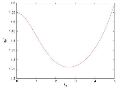
Figure 5: Plot showing how the Reynolds number at onset varies with $k_{x}$ for $P=50$, $E=10^{-4}$, $Ra=-1$ and $k_{y}=k_{y_{c}}=0$ with stress-free boundaries.

3.4 Thermodynamic equation

To form the energy equation we consider the dot product of $\mathbf{u}$ with equation (8) and integrate over the volume of the layer. In the limit $k_{y}=0$, the situation most favourable to baroclinic instability, the only terms that remain are the balance of the work done by buoyancy and the rate of working of the viscous forces,

$$Ra\int u_{z}\theta\,dV=\int\frac{\partial u_{i}}{\partial x_{j}}\frac{\partial u_{i}}{\partial x_{j}}\,dV,$$ (22)

where we have non-dimensionalised using the same scales as earlier. Following chapter 2 of Chandrasekhar (1961), we now multiply the temperature equation (9) by $\theta$ and eliminate the rate of working of the buoyancy force to obtain the thermodynamic equation

$$Ra\int(\nabla\theta)^{2}dV-PE^{-1}Re\int\theta u_{y}dV-\int\frac{\partial u_{i}}{\partial x_{j}}\frac{\partial u_{i}}{\partial x_{j}}dV=0,\quad{\rm or}\quad I_{1}+I_{2}+I_{3}=0.$$ (23)

The second integral, $I_{2}$, is related to the heat flux carried in the $y$ direction, and is only non-zero when the zonal flow is non-zero. The third term, $I_{3}$, is the rate of viscous dissipation. We can write this equation in terms of the real and imaginary parts of $u_{z}$, $\omega_{z}$ and $\theta$ and their derivatives, all of which have been calculated in the numerics above. Figure 6 shows how the three terms in equation (23) vary as a function of $Re$ for a specific choice of $k_{x}$. Plots for other $k_{x}$ where baroclinic modes exist are similar with the position of the transition region changing accordingly.

Since the integral in the first term is positive definite, and that in the third term is negative definite, we must also have $Ra>0$ in the case $Re=0$. This is the well understood case where the Rayleigh number must be positive for the system to be convectively unstable. At low $Re$ this remains the predominant balance and the Rayleigh number remains positive. However with $Re\neq 0$ the baroclinic term can now partially balance the viscous stresses and thus as $Re$ is increased the Rayleigh number is reduced to allow equation (23) to balance. This can be seen in figure 6 where the $I_{2}$ contribution slowly increases in magnitude as $Re$ increases.

As $Re$ is increased further and we enter the transition region (located at $Re\sim 19.86$ for $k_{x}=5.0119$) we see that both $I_{1}$ and the baroclinic flux, $I_{2}$, change sign. In the transition region the main balance is between these two terms as the magnitude of the rate of working of the viscous stresses is small. However the sum of $I_{1}$ and $I_{2}$ must still balance the always negative $I_{3}$ term. The transition region represents the point in $Re$-space where $I_{2}$ becomes large enough in magnitude to solely overcome $I_{3}$ without the need for a contribution from $I_{1}$. Hence $I_{1}$ can change sign, so that $Ra$ must change sign also. This explains why a sufficiently large value of the zonal wind is required to allow for modes with negative Rayleigh number to appear. It also indicates that the term, $I_{1}$ or $I_{2}$, in equation (23) which is positive, and thus is able to balance $I_{3}$, contains the parameter that is driving the instability. In other words it is the Rayleigh/Reynolds number and thus the work done by buoyancy/baroclinic heat flux, which is balancing the viscous dissipation in the convective/baroclinic regime.

Equation (23) can also explain the results of changing the Prandtl number given by table 2. Since $I_{2}$ in the thermodynamic equation is proportional to $P$, increasing or decreasing the Prandtl number requires a lower or higher value of $Re$ respectively. This is slightly crude since it assumes that the values of the integrals in equation (23) do not change with $P$. This is not the case, which is why increasing the Prandtl number by an order of magnitude does not result in the zonal wind decreasing by the same amount. For example the position of the transition region for $P=10$ in table 2 has only moved from $Re\sim 10$ (in the $P=1$ case) to $Re\sim 3.5$ rather than $Re\sim 1$. Despite this the form of $I_{2}$ in the thermodynamic equation serves to explain the general dependency of the transition region on $P$.

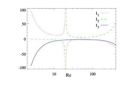
Figure 6: Plot showing how the integrals in the thermodynamic equation (23) vary with $Re$, at $E=10^{-4}$. There are stress-free boundaries and $P=1$, $k_{x}=5.0119$ and $k_{y}=k_{y_{c}}=0$.

4 Asymptotics

Here we develop asymptotic theories, which predict the numeric results with stress-free boundaries very well. In the numerical work previously discussed we have been considering low but finite values of the Ekman number since these are of particular physical interest. Hence the first limit to take is that of asymptotically small $E$. Guided by the numerics we rescale the dependent variables as $\omega_{z}={\tilde{\omega}_{z}}$, $u_{z}=E{\tilde{u}_{z}}$, $\theta=E{\tilde{\theta}}$, and $Ra=-{\tilde{R}}/E^{2}$ and then we find that the leading order equations from (17) - (19) in the limit $E\to 0$ are

$$\left(\sigma+\mathrm{i}k_{x}Rez+k^{2}-\frac{\mathrm{d}^{2}}{\mathrm{d}z^{2}}\right){\tilde{\omega}_{z}}=\frac{\mathrm{d}{\tilde{u}_{z}}}{\mathrm{d}z},$$ (24)

$$\frac{\mathrm{d}{\tilde{\omega}_{z}}}{\mathrm{d}z}=k^{2}{\tilde{R}}{\tilde{\theta}},$$ (25)

$$\left(\sigma+\mathrm{i}k_{x}PRez+k^{2}-\frac{\mathrm{d}^{2}}{\mathrm{d}z^{2}}\right){\tilde{\theta}}={\tilde{u}_{z}}+\frac{\mathrm{i}k_{x}PRe}{k^{2}{\tilde{R}}}{\tilde{\omega}_{z}}.$$ (26)

From these equations we are able to easily eliminate $\tilde{\theta}$ by taking the double-derivative of equation (25) and substituting into equation (26) to give

$$\frac{\mathrm{d}^{3}{\tilde{\omega}_{z}}}{\mathrm{d}z^{3}}=(\sigma+\mathrm{i}k_{x}PRez+k^{2})\frac{\mathrm{d}{\tilde{\omega}_{z}}}{\mathrm{d}z}-\mathrm{i}k_{x}PRe{\tilde{\omega}_{z}}-\tilde{R}k^{2}\tilde{u}_{z}.$$ (27)

We use equations (24) - (27) in each of our asymptotic theories and thus they are only accurate for low Ekman numbers. These equations are related to the quasi-geostrophic equations used by atmospheric scientists, see section 4.3 below, though here diffusion is still included.

4.1 Low wavenumber asymptotics 1: Fixed Rayleigh number

In this theory we obtain an expression for the critical Reynolds number in terms of the Prandtl and Rayleigh numbers. We set $\sigma=0$ because we are considering steady marginal modes and since the critical latitudinal wavenumber vanishes for all modes of interest we also set $k_{y}=k_{y_{c}}=0$ so that $k=k_{x}$. The numerics suggest that the critical azimuthal wavenumber is zero for baroclinic modes and thus we expand $\tilde{\omega}_{z}$, $\tilde{u}_{z}$ and $Re$ in powers of the small parameter $k$ as follows:

$${\tilde{\omega}_{z}} = 1+k\omega_{1}+k^{2}\omega_{2}+\cdots,$$ (28)

$${\tilde{u}_{z}} = k(u_{0}+ku_{1}+k^{2}u_{2}+\cdots),$$ (29)

$$Re = Re_{0}+kRe_{1}+k^{2}Re_{2}+\cdots.$$ (30)

We have chosen $\omega_{0}=1$ to satisfy normalisation conditions and in this theory we apply the stress-free boundary conditions given by equation (20). It is also useful to take the integral of equation (24) across the layer since the boundary conditions eliminate two of the resulting terms to leave

$$\int_{-1/2}^{1/2}(\mathrm{i}kRez+k^{2})\tilde{\omega}_{z}\mathrm{d}z=0.$$ (31)

We now proceed by considering the equations at increasing order (i.e. powers of $k$). Equations (27) and (24) at order $\mathrm{O}(k)$ give

$$\frac{\mathrm{d}^{3}\omega_{1}}{\mathrm{d}z^{3}}=-\mathrm{i}PRe_{0},$$ (32)

$$\mathrm{i}Re_{0}z-\frac{\mathrm{d}^{2}\omega_{1}}{\mathrm{d}z^{2}}=\frac{\mathrm{d}u_{0}}{\mathrm{d}z}$$ (33)

respectively, which when applying the boundary conditions gives

$$\omega_{1}=-\mathrm{i}PRe_{0}\left(\frac{z^{3}}{6}-\frac{z}{8}\right),$$ (34)

$$u_{0}=\mathrm{i}Re_{0}(1+P)\left(\frac{z^{2}}{2}-\frac{1}{8}\right).$$ (35)

Next we consider equations (31) and (27) at $\mathrm{O}(k^{2})$ to give

$$\int_{-1/2}^{1/2}(\mathrm{i}Re_{0}z\omega_{1}+\mathrm{i}Re_{1}z+1)\mathrm{d}z=0,$$ (36)

$$\frac{\mathrm{d}^{3}\omega_{2}}{\mathrm{d}z^{3}}=\mathrm{i}PRe_{0}z\frac{\mathrm{d}\omega_{1}}{\mathrm{d}z}-\mathrm{i}PRe_{0}\omega_{1}-\mathrm{i}PRe_{1}$$ (37)

and by using the definition of $\omega_{1}$ we can evaluate the integral in equation (36) to acquire

$$Re_{0}=\sqrt{\frac{120}{P}}.$$ (38)

We can also find $\omega_{2}$ from equation (37) by inserting the definition of $\omega_{1}$ and using the boundary conditions to get

$$\omega_{2}=P^{2}Re_{0}^{2}\left(\frac{z^{6}}{360}-\frac{z^{2}}{1920}\right)-\mathrm{i}PRe_{1}\left(\frac{z^{3}}{6}-\frac{z}{8}\right).$$ (39)

Once again considering equations (31) and (27), now at $\mathrm{O}(k^{3})$, we obtain

$$\int_{-1/2}^{1/2}(\mathrm{i}Re_{0}z\omega_{2}+\mathrm{i}Re_{1}z\omega_{1}+\mathrm{i}Re_{2}z+\omega_{1})\mathrm{d}z=0,$$ (40)

$$\frac{\mathrm{d}^{3}\omega_{3}}{\mathrm{d}z^{3}}=\mathrm{i}PRe_{0}z\frac{\mathrm{d}\omega_{2}}{\mathrm{d}z}+\mathrm{i}PRe_{1}z\frac{\mathrm{d}\omega_{1}}{\mathrm{d}z}+\frac{\mathrm{d}\omega_{1}}{\mathrm{d}z}-\mathrm{i}PRe_{0}\omega_{2}-\mathrm{i}PRe_{1}\omega_{1}-\mathrm{i}PRe_{2}-\tilde{R}u_{0}$$ (41)

respectively whereby $Re_{1}=0$ to satisfy equation (40). By inserting the definitions of $\omega_{1}$, $\omega_{2}$ and $u_{0}$ into equation (41) we find

$$\omega_{3}=\mathrm{i}P^{3}Re_{0}^{3}\left(\frac{z^{9}}{36288}-\frac{z^{5}}{115200}+\frac{z}{573440}\right)-\mathrm{i}Re_{0}(P+\tilde{R}(1+P))\left(\frac{z^{5}}{120}-\frac{z^{3}}{48}+\frac{5z}{384}\right)-\mathrm{i}PRe_{2}\left(\frac{z^{3}}{6}-\frac{z}{8}\right).$$ (42)

We are now able to find an expression for $Re_{2}$ using equation (31) at $\mathrm{O}(k^{4})$, which is

$$\int_{-1/2}^{1/2}(\mathrm{i}Re_{0}z\omega_{3}+\mathrm{i}Re_{2}z\omega_{1}+\mathrm{i}Re_{3}z+\omega_{2})\mathrm{d}z=0.$$ (43)

We insert the expressions for $\omega_{1}$, $\omega_{2}$ and $\omega_{3}$ into equation (43) and evaluate the integral to find

$$Re_{2}=\sqrt{\frac{30}{P}}\left[\frac{17}{168}\left(1+\frac{\tilde{R}(1+P)}{P}\right)-\frac{5P}{792}\right].$$ (44)

Hence from equation (30) we find

$$Re\approx Re_{0}+k^{2}Re_{2}=\sqrt{\frac{120}{P}}+k^{2}\sqrt{\frac{30}{P}}\left[\frac{17}{168}\left(1+\frac{\tilde{R}(1+P)}{P}\right)-\frac{5P}{792}\right],$$ (45)

which yields an approximation to the Reynolds number given $P$, $\tilde{R}$ and a small $k$. The form of this expression for $Re$ is able to explain the dependence of the critical wavenumber on $P$ as seen in section 3.3. For a given Prandtl number the $Re_{0}$ term in the expression for $Re$ given by (45) gives an approximation to the critical Reynolds number. For example with $P=1$ this term is $\sim 10.9545$, which is in excellent agreement with the numerics discussed in section 3.2. The second term of equation (45) then gives an adjustment to the the leading order value for $Re$. The sign of this term determines whether $k_{c}=0$ or not. If, for a given $P$ and $\tilde{R}$, the value of $Re_{2}$ is positive then the adjustment to $Re_{0}$ can only serve to increase the Reynolds number and hence the preferred value of $k$ to minimise $Re$ is $k=0$ as expected given the numeric results from section 3.2. However if the value of $Re_{2}$ is negative (again for given $P$ and $\tilde{R}$) a non-zero $k$ must be preferred as the inclusion of this term now lowers the Reynolds number from the $Re_{0}$ value.

Table 3 displays quantities for $Re_{0}$ and $Re_{2}$ for various values of $P$ and $\tilde{R}$. Since $Re_{0}$ is independent of $\tilde{R}$ this only varies with $P$ and the values predicted for the Reynolds number match the numerics of table 2 very well. For most combinations of $P$ and $\tilde{R}$ the value of $Re_{2}$ is positive, confirming that $k_{c}=0$ and $Re_{c}=Re_{0}$. However for certain choices of the parameters we obtain negative values for $Re_{2}$ indicating that there is a non-zero minimising value of $k$. This was seen in the numerics where we recall from figure 5 that there was a non-zero $k_{c}$ for $P=50$ and $Ra=-1$. The equivalent values of the Prandtl and Rayleigh numbers in the asymptotic theory ($P=50$ and $\tilde{R}=1$) give a negative value of $Re_{2}$ agreeing with the numerics that there is a non-zero minimising $k$.

		$Re_{2}$
$P$	$Re_{0}$	$\tilde{R}=0$	$\tilde{R}=1$	$\tilde{R}=10$	$\tilde{R}=1000$
0.1	$34.64102$	$1.74174$	$21.02111$	$194.53549$	$19281.11679$
1	$10.95445$	$0.51966$	$1.62815$	$11.60453$	$1109.00579$
10	$3.46410$	$0.065920$	$0.25871$	$1.99386$	$192.85967$
50	$1.54919$	$-0.16612$	$-0.086175$	$0.63337$	$79.78332$
100	$1.09545$	$-0.29036$	$-0.23438$	$0.26943$	$55.68819$

Table 3: Table displaying values for $Re_{0}$ and $Re_{2}$ for various Prandtl and Rayleigh numbers as given by the expression in equation (45).

This theory is unable to predict the critical wavenumber and critical Reynolds number when $Re_{2}<0$ without including higher order terms, which would give an $\mathrm{O}(k^{4})$ term in equation (45). However it does indicate which values of the Prandtl and Rayleigh numbers we would expect to find a non-zero critical wavenumber for and it predicts $Re_{c}$ very accurately for the $k_{c}=0$ cases.

We are also able to solve equations (24) and (27) numerically without the assumption of small $k$. Using stress-free boundary conditions and the normalisation and symmetry conditions of the eigenfunctions (known from the numerics) we have a fourth order complex BVP with nine real boundary conditions, including a normalisation condition,

$$\omega_{\mathrm{r}}(0)=1,\ \ \omega_{\mathrm{i}}(0)=\omega_{\mathrm{r}}^{\prime}(0)=\omega_{\mathrm{i}}^{\prime\prime}(0)=u_{\mathrm{r}}(0)=0,\ \ \omega_{\mathrm{r}}^{\prime}(0.5)=\omega_{\mathrm{i}}^{\prime}(0.5)=u_{\mathrm{r}}(0.5)=u_{\mathrm{i}}(0.5)=0.$$ (46)

Here the primes and subscripts indicate the derivatives and the real and imaginary parts of the eigenfunctions respectively. The system defined by (24), (27) and (46) is an eighth order homogeneous system in the real variables, with eight homogeneous boundary conditions and a normalisation condition, so it has an eigenvalue, $Re$. Hence given specific values of $k$, $P$ and $\tilde{R}$ we can find a value for $Re$. We solved this system using a simple BVP solver in Maple and some results for the case of $\tilde{R}=0$ are displayed in table 4(a). By comparing the values of $Re$ in table 4(a) with the location of the transition region from figure 1(a) and table 2 we see that the asymptotic theory predicts the location of the transition region very well. In particular, we see that the position of the transition region is converging, as we reduce $E$, to a value similar to that predicted by the asymptotics in all cases. Also of note is that for $P=20$ and $P=50$ there are minimising values of the azimuthal wavenumber due to the fact that the Rayleigh number is small enough to allow this to occur. In fact this can be checked by evaluating $Re_{2}$ as given by equation (45) with $\tilde{R}=0$ where we indeed find that $Re_{2}<0$ for $P=20$ and $P=50$, indicating a non-zero critical wavenumber is preferred.

	$Re$
$k_{x}$	$P=0.1$	$P=1$	$P=10$	$P=20$	$P=50$
0.01	$34.64108$	$10.95447$	$3.46410$	$2.44948$	$1.54917$
0.10	$34.65831$	$10.95961$	$3.46475$	$2.44918$	$1.54754$
0.50	$35.07369$	$11.08347$	$3.48056$	$2.44245$	$1.51100$
1.00	$36.34019$	$11.46042$	$3.52963$	$2.42794$	$1.42646$
1.50	$38.35637$	$12.05843$	$3.61070$	$2.42013$	$1.34371$
2.00	$41.00963$	$12.84220$	$3.72316$	$2.43154$	$1.28719$
2.50	$44.18317$	$13.77610$	$3.86686$	$2.46939$	$1.26193$
3.00	$47.77158$	$14.82920$	$4.04217$	$2.53699$	$1.26634$
5.00	$64.77836$	$19.83002$	$5.08823$	$3.14797$	$1.59143$
10.0	$114.69132$	$35.11997$	$10.51240$	$7.57080$	$4.80621$

$Re$	$k_{y}/k_{x}$	$R_{0}$
10	0	0.8983
	0.001	0.8987
	0.01	0.9377
100	0	-9.6578
	0.001	-9.5599
	0.01	-4.7143
1000	0	-9.8903
	0.001	-4.9440
	0.01	-0.09560
10000	0	-9.8926
	0.001	-0.09792
	0.01	-9.6568$\times 10^{-4}$

Table 4: Tables displaying results from the two asymptotic theories described in section 4. 4(a): Values for the Reynolds number for various $k_{x}$ and $P$ in the case $\tilde{R}=0$ found by solving the BVP described by equations (24) and (27). 4(b): Values for $R_{0}$ found by solving equation (66) for various values of $Re$ and $k_{y}/k_{x}$ with $P=1$.

4.2 Low wavenumber asymptotics 2: Fixed Reynolds number

Here we shall develop an asymptotic theory for the onset of instability at low $k_{x}$ with stress-free boundaries, which predicts the large negative Rayleigh numbers and eigenfunctions very well. Our starting point is equations (24) - (26) with the boundary conditions given by (20). We set $\sigma=0$ for the same reason as in section 4.1. The numerics inform us that the baroclinic modes exist for small $k_{x}Re$ and that we should rescale the Rayleigh number as $\tilde{R}=-{\hat{R}}/k_{x}^{2}$. The equations (24) - (26) become

$$\left(\mathrm{i}k_{x}Rez+k^{2}-\frac{\mathrm{d}^{2}}{\mathrm{d}z^{2}}\right){\tilde{\omega}_{z}}-\frac{\mathrm{d}{\tilde{u}_{z}}}{\mathrm{d}z}=0,$$ (47)

$$\frac{\mathrm{d}{\tilde{\omega}_{z}}}{\mathrm{d}z}=-{\hat{R}}{\tilde{\theta}},$$ (48)

$$\left(\mathrm{i}k_{x}PRez+k^{2}-\frac{\mathrm{d}^{2}}{\mathrm{d}z^{2}}\right){\tilde{\theta}}={\tilde{u}_{z}}-\frac{\mathrm{i}k_{x}PRe}{{\hat{R}}}{\tilde{\omega}_{z}}.$$ (49)

We introduce a small parameter $\epsilon$, measuring the magnitude of the horizontal wavenumbers, and let

$${\tilde{\omega}_{z}} = \omega_{z}^{(0)}+\epsilon\omega_{z}^{(1)}+\epsilon^{2}\omega_{z}^{(2)}+\cdots,$$ (50)

$${\tilde{u}_{z}} = \epsilon(u_{z}^{(0)}+\epsilon u_{z}^{(1)}+\epsilon^{2}u_{z}^{(2)}+\cdots),$$ (51)

$${\tilde{\theta}} = \epsilon(\theta^{(0)}+\epsilon\theta^{(1)}+\epsilon^{2}\theta^{(2)}+\cdots),$$ (52)

$${\hat{R}} = R_{0}+\epsilon R_{1}+\epsilon^{2}R_{2}+\cdots,$$ (53)

$$k_{x} = \epsilon{\tilde{k}_{x}},\qquad k_{y}=\epsilon{\tilde{k}_{y}},$$ (54)

where we assume that $R_{0}<0$ since we are considering the stably stratified modes in this asymptotic expansion.

We insert these expansions into equations (47) - (49) and consider the resulting equations in powers of $\epsilon$ since $k_{x}\ll 1$. Hence we first take each equation at $\mathrm{O}(1)$, which yields

$$\omega_{z}^{(0)}=1.$$ (55)

This choice of $\omega_{z}^{(0)}$ satisfies this set of equations and is chosen to be unity to satisfy normalisation conditions. Also note that this form for $\omega_{z}^{(0)}$ satisfies the stress-free boundary conditions on $\omega_{z}$ given by (20), and so no thin boundary layer to match these conditions is required.

Next we consider the first order equations, which are equations (47) - (49) at $\mathrm{O}(\epsilon)$ and we find:

$$\mathrm{i}{\tilde{k}_{x}}Rez\omega_{z}^{(0)}-\frac{\mathrm{d}^{2}\omega_{z}^{(1)}}{\mathrm{d}z^{2}}=\frac{\mathrm{d}u_{z}^{(0)}}{\mathrm{d}z},$$ (56)

$$\frac{\mathrm{d}\omega_{z}^{(1)}}{\mathrm{d}z}=-R_{0}\theta^{(0)},$$ (57)

$$-\frac{\mathrm{d}^{2}\theta^{(0)}}{\mathrm{d}z^{2}}=u_{z}^{(0)}-\frac{\mathrm{i}{\tilde{k}_{x}}ReP\omega_{z}^{(0)}}{R_{0}}.$$ (58)

We integrate (56) and apply the no penetration and zero temperature boundary conditions, using (48), to obtain the constant of integration, and insert the expression for $u_{z}^{(0)}$ into (58) to obtain

$$\frac{\mathrm{d}^{2}\theta^{(0)}}{\mathrm{d}z^{2}}+R_{0}\theta^{(0)}=-\frac{\mathrm{i}{\tilde{k}_{x}}Rez^{2}}{2}+\frac{\mathrm{i}{\tilde{k}_{x}}Re}{8}+\frac{\mathrm{i}{\tilde{k}_{x}}ReP}{R_{0}}.$$ (59)

The solution to this inhomogeneous second order ODE in $\theta^{(0)}$ is

$$\theta^{(0)}=A\sinh\left(\sqrt{-R_{0}}z\right)+B\cosh\left(\sqrt{-R_{0}}z\right)-\frac{\mathrm{i}{\tilde{k}_{x}}Rez^{2}}{2R_{0}}+\gamma.$$ (60)

Due to the symmetry of the boundary conditions $A=0$ so in fact

$$\theta^{(0)} = B\cosh\left(\sqrt{-{R}_{0}}z\right)-\frac{\mathrm{i}{\tilde{k}_{x}}Rez^{2}}{2{R}_{0}}+\gamma,$$ (61)

$$u_{z}^{(0)} = B{R}_{0}\cosh\left(\sqrt{-{R}_{0}}z\right)+\frac{\mathrm{i}{\tilde{k}_{x}}Re}{R_{0}}(1+P),$$ (62)

$$\omega_{z}^{(1)} = B\sqrt{-{R}_{0}}\sinh\left(\sqrt{-{R}_{0}}z\right)+\frac{\mathrm{i}{\tilde{k}_{x}}Rez^{3}}{6}-{R}_{0}\gamma z,$$ (63)

where the expressions for $u_{z}^{(0)}$ and $\omega_{z}^{(1)}$ have been found via equations (58) and (57) respectively. Any constant of integration in (63) can be absorbed in the normalisation condition (55). We can also determine $B$ and $\gamma$ by considering the no penetration and zero temperature boundary conditions on these expressions for $u_{z}^{(0)}$ and $\theta^{(0)}$. We find that both $B$ and $\gamma$ are purely imaginary:

$$B=\frac{-\mathrm{i}{\tilde{k}_{x}}Re(1+P)}{{R}_{0}^{2}\cosh\left(\sqrt{-{R}_{0}}/2\right)}\qquad\text{and}\qquad\gamma=\mathrm{i}{\tilde{k}_{x}}Re\left(\frac{1+P}{{R}_{0}^{2}}+\frac{1}{8{R}_{0}}\right).$$ (64)

With these expressions for $B$ and $\gamma$ we have acquired the complete expressions for $\omega_{z}^{(1)}$, $u_{z}^{(0)}$ and $\theta^{(0)}$.

Thus we now look at the next order of equation (47). At $\mathrm{O}(\epsilon^{2})$ we find

$$\mathrm{i}{\tilde{k}_{x}}Rez\omega_{z}^{(1)}+{\tilde{k}_{x}}^{2}+{\tilde{k}_{y}}^{2}-\frac{\mathrm{d}^{2}\omega_{z}^{(2)}}{\mathrm{d}z^{2}}=\frac{\mathrm{d}u_{z}^{(1)}}{\mathrm{d}z}.$$ (65)

When taking the boundary conditions on the integral of this equation the final two terms will vanish since $\mathrm{d}\omega_{z}/\mathrm{d}z=0=u_{z}$ on the boundary. Therefore if we consider the integral of this equation over the layer, substitute for $\omega_{z}^{(1)}$ and $B$ and $\gamma$ from equations (63) and (64) respectively and apply the boundary conditions we obtain

$$\frac{1+P}{{R}_{0}^{2}}-\frac{2(1+P)\tanh\left(\sqrt{-{R}_{0}}/2\right)}{\sqrt{-{R}_{0}}{R}_{0}^{2}}+\frac{1+P}{12{R}_{0}}+\frac{1}{120}+\frac{1}{Re^{2}}\left(1+\frac{k_{y}^{2}}{k_{x}^{2}}\right)=0.$$ (66)

Equation (66) can be solved numerically for $R_{0}$ using given values of the parameters, $P$, $Re$ and $k_{y}/k_{x}$.

If we first consider the case $P=1$, $k_{y}/k_{x}=0$ and $Re=100$ we can compare the numeric results given by table 1 with those of table 4(b). We find that the asymptotics predict the numerics very well. For example at asymptotically small azimuthal wavenumber table 1 predicts that the Rayleigh number at onset will tend towards the value $-9.6577E^{-2}k_{x}^{-2}$. We see from table 4(b) that this gives excellent agreement. For modes with $k_{y}/k_{x}=0$ the asymptotics predict that $R_{0}$ is converging to approximately $-9.9$ with increasing zonal flow, which is also in excellent agreement with the numerics. Also of note is that equation (66) has no negative $R_{0}$ solutions for $Re<10.9496$. As a result of this the asymptotic results, in table 4(b), predict only modes with $R_{0}>0$ for $Re=10$. This is in excellent agreement with the numerics as the baroclinic modes were found to ‘switch-off’ for approximately $Re<10.95$.

We can also see that the asymptotics of table 4(b) predict that increasing $k_{y}$ only serves to stabilise the system by increasing the Rayleigh number at onset in all cases. This matches the numerics as described in section 3.3. In figure 7 we have plotted the eigenfunctions predicted by the lowest order asymptotics as given by equations (55), (61) and (62) scaled using $u_{z}=E{\tilde{u}_{z}}$, $\theta=E{\tilde{\theta}}$ in order to compare with the equivalent parameter values at point $\times_{2}$ from figure 1(a). By comparing this plot with that of 2(b) we can clearly see that the low wavenumber asymptotic theory is also predicting the correct form and magnitude of the eigenfunctions. The asymptotics continue to predict the correct form of the eigenfunctions for larger values of the Reynolds number where the onset parameter becomes the Rayleigh number, $Ra^{*}$.

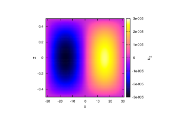
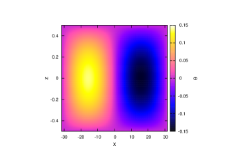
Figure 7: Eigenfunction plots as predicted by the low wavenumber asymptotic theory. This is the equivalent of point $\times_{2}$ from figure 1(a) where $E=10^{-4}$, $P=1$, $Ra=-10^{6}$, $Re=Re^{*}\equiv 10.9599$, $k_{x}=0.1$ and $k_{y}=k_{y_{c}}=0$.

4.3 Relation to the Eady problem

The low wavenumber equations (47) - (49) are related to the quasi-geostrophic (QG) equations used in atmospheric science (see e.g. Pedlosky, 1987). The geostrophic component of the velocity is given by $2\Omega(u_{x}^{G},u_{y}^{G})=(-\partial p/\partial y,\partial p/\partial x)$, so $\omega_{z}=-k^{2}p/2\Omega$, and the pressure perturbation is simply proportional to the vertical vorticity, and so equation (48) is simply the hydrostatic equation used in the QG approximation, where vertical accelerations are neglected. The $y$-derivative terms in equations (10) and (12) are also dropped in the Eady problem (see e.g. Drazin and Reid, 1981, p333) because of the low Rossby number assumption, here $ReE<<1$. If we take the $z$-derivative of (49) and eliminate $\tilde{u}_{z}$ and $\tilde{\theta}$ using (47) and (48), we obtain

$$\left(\sigma P+\mathrm{i}k_{x}PRez+k^{2}-\frac{\mathrm{d}^{2}}{\mathrm{d}z^{2}}\right)\frac{\mathrm{d}^{2}{\tilde{\omega}_{z}}}{\mathrm{d}z^{2}}+\left(\sigma+\mathrm{i}k_{x}Rez+k^{2}-\frac{\mathrm{d}^{2}}{\mathrm{d}z^{2}}\right){\hat{R}}{\tilde{\omega}_{z}}=0.$$ (67)

In the QG approximation, diffusion is usually ignored, and so the terms $k^{2}-\mathrm{d}^{2}/\mathrm{d}z^{2}$ are dropped in (67), leading to the classical Eady equation

$$\left(\sigma+\mathrm{i}k_{x}Rez\right)\left(\frac{\mathrm{d}^{2}{\tilde{\omega}_{z}}}{\mathrm{d}z^{2}}+\frac{{\hat{R}}}{P}{\tilde{\omega}_{z}}\right)=0,$$ (68)

see e.g. equation (4.5.28) of Drazin and Reid (1981). The only boundary condition to survive the neglect of diffusion is $\tilde{u}_{z}=0$, which leads to

$$\left(\sigma+\mathrm{i}k_{x}Rez\right)\frac{\mathrm{d}{\tilde{\omega}_{z}}}{\mathrm{d}z}=\mathrm{i}k_{x}PRe{\tilde{\omega}_{z}},\quad{\rm on}\quad z=\pm\frac{1}{2},$$ (69)

equivalent to equation (4.5.30) of Drazin and Reid (1981). Instability occurs as an oscillatory mode, $\Im[\sigma]\neq 0$. The relevant part of our parameter space is where $Re$ is large, since the viscosity is small, and there we found oscillatory baroclinic modes as in figure 2(c), point $\times_{3}$.

5 Conclusions

The way in which convective instability and baroclinic instability interact in rapidly rotating systems has been elucidated. We found that the thermal wind destabilises convective modes, lowering the critical Rayleigh number at which they onset. We also find that the critical azimuthal wavelength at onset lengthens. At a sufficiently large Reynolds number, which in view of the very small viscosity occurring in many geophysical systems can correspond to a rather small thermal wind, instability becomes predominantly baroclinic, and the preferred azimuthal wavenumber tends to zero. In our ideal plane layer geometry, there is no restriction on possible wavelengths, but in more realistic spherical geometries, the boundaries will provide a limit. Slightly to our surprise, we found that convective modes and baroclinic modes are smoothly connected, going through a transition region which can be studied asymptotically (section 4.1) where the critical Rayleigh number smoothly goes between positive and negative values. At the low azimuthal wavenumbers preferred by baroclinic modes, an asymptotic analysis is possible (section 4.2) which gives good agreement with the numerics in the stress-free case, and illuminates which terms are important for instability. We also found that generally waves with non-zero latitudinal wavenumber $k_{y}$ are not preferred in this problem, onset occurring in all cases examined at the lowest $Ra$ when $k_{y}=0$.

At moderate Prandtl numbers, the onset of convection in this rotating Bénard configuration occurs with steady modes, but we find that at large Reynolds number oscillatory modes are preferred. This result links our finite diffusion work with the quasi-geostrophic shallow layer approximation used in atmospheric science, and in particular with the Eady problem (section 4.3).

The existence of baroclinic instability in the physical conditions obtaining in planetary interiors raises an interesting question of whether dynamo action could be driven by a heterogeneous core-mantle heat flux even if the core is stably stratified. This has also been investigated by Sreenivasan (2009) where lateral variations were found to support a dynamo even when convection is weak. It is widely believed that the heat flux passing from the Earth’s core to its mantle can vary by order one amounts with latitude and longitude, as a result of cool slabs descending through the mantle and reaching the CMB from above. It is also generally believed that the key criterion for the existence of a dynamo is that convection should be occurring, and that the core is at least on average unstably stratified. However, this analysis has raised the possibility that instabilities leading to fluid motion driven by lateral temperature gradients can occur even when the fluid is strongly stably stratified. Of course, it is not yet known whether the resulting nonlinear motions would be suitable for driving a dynamo. In the plane layer geometry used here, the preferred motion appears to be two-dimensional and therefore will not drive a dynamo. However, in spherical geometry, and when secondary instabilities may occur, dynamo action may become possible, in which case the view that convection driven by an unstable temperature gradient is essential for dynamo action might have to be revised.

References

- Anufriev et al. (2005) Anufriev, A., Jones, C. and Soward, A., The Boussinesq and anelastic liquid approximations for convection in the Earth’s core. Phys. Earth Planet. Inter. 2005, 152, 163–190.
- Aurnou et al. (2003) Aurnou, J., Andreadis, S., Zhu, L. and Olson, P., Experiments on convection in the Earth’s core tangent cylinder. Earth Planet. Sci. Lett. 2003, 212, 119–134.
- Braginsky (1993) Braginsky, S., MAC-oscillations of the hidden ocean of the core. J. Geomagn. Geoelectr. 1993, 45, 1517–1538.
- Busse (1970) Busse, F., Thermal instabilities in rapidly rotating systems. J. Fluid Mech. 1970, 44, 441–460.
- Busse and Carrigan (1976) Busse, F. and Carrigan, C., Laboratory simulation of thermal convection in rotating planets and stars. Science. 1976, 191, 81–83.
- Chandrasekhar (1961) Chandrasekhar, S., Hydrodynamic and Hydromagnetic Stability, 1961 (Oxford, Clarendon Press.).
- Dormy et al. (2004) Dormy, E., Soward, A., Jones, C., Jault, D. and Cardin, P., The onset of thermal convection in rotating spherical shells. J. Fluid Mech. 2004, 501, 43–70.
- Drazin and Reid (1981) Drazin, P. and Reid, W., Hydrodynamic stability, 1981 (Cambridge University Press).
- Gubbins et al. (2007) Gubbins, D., Willis, A. and Sreenivasan, B., Correlation of Earth’s magnetic field with lower mantle thermal and seismic structure. J. Fluid Mech. 2007, 162, 256–260.
- Jones (2000) Jones, C., Convection driven geodynamo models. Phil. Trans. R. Soc. Lond. A 2000, 358, 873–897.
- Jones et al. (2000) Jones, C., Soward, A. and Mussa, A., The onset of convection in a rapidly rotating sphere. J. Fluid Mech. 2000, 405, 157–179.
- Olson and Aurnou (1999) Olson, P. and Aurnou, J., A polar vortex in the Earth’s core. J. Geophys. Res. 1999, 402, 170–173.
- Olson et al. (1999) Olson, P., Christensen, U. and Glatzmaier, G., Numerical modeling of the geodynamo: mechanisms of field generation and equilibration. J. Geophys. Res. 1999, 104, 10383–10404.
- Pedlosky (1987) Pedlosky, J., Geophysical Fluid Dynamics, 1987 (Springer).
- Roberts (1968) Roberts, P., On the thermal instability of a rotating fluid sphere containing heat sources. Phil. Trans. R. Soc. Lond. A 1968, 263, 93–117.
- Sreenivasan (2009) Sreenivasan, B., On dynamo action produced by boundary thermal coupling. Phys. Earth Planet. Inter. 2009, 177, 130–138.
- Sreenivasan and Jones (2005) Sreenivasan, B. and Jones, C., Structure and dynamics of the polar vortex in the Earth’s core. Geophys. Res. Lett. 2005, 32, L20301.
- Sreenivasan and Jones (2006) Sreenivasan, B. and Jones, C., Azimuthal winds, convection and dynamo action in the polar region of the planetary cores. Geophys. Astrophys. Fluid Dynam. 2006, 100, 319–339.
- Tilgner and Busse (1997) Tilgner, A. and Busse, F., Finite-amplitude convection in rotating spherical fluid shells. J. Fluid. Mech. 1997, 332, 359–376.
- Zhang (1992) Zhang, K., Spiralling columnar convection in rapidly rotating spherical shells. J. Fluid Mech. 1992, 236, 535–556.
- Zhang and Gubbins (1996) Zhang, K. and Gubbins, D., Convection in a rotating sphericalfluid shell with an inhomogeneous temperature boundary condition at finitePrandtl number. Phys. Fluids 1996, 8, 1141–1158.