Study of the thermal abelian monopoles with proper gauge fixing

Abstract

The properties of the thermal abelian monopoles are studied in the deconfinement phase of the $SU(2)$ gluodynamics. To remove effects of Gribov copies the simulated annealing algorithm is applied to fix the maximally abelian gauge. Computing the density of the thermal abelian monopoles in the temperature range between $1.5~{}T_{c}$ and $6.9~{}T_{c}$ we show, by comparison with earlier results, that the Gribov copies effects might be as high as 20% making proper gauge fixing mandatory. We find that in the infinite temperature limit the monopole density converges to its value in 3-dimensional theory. To study the interaction between monopoles we calculate the monopole-monopole and monopole-antimonopole correlators at different temperatures in the region $(1.5~{}T_{c},6.9~{}T_{c})$. Using the result of this study we determine the screening mass, monopole-monopole coupling constant, monopole size and monopole mass. In addition we check the continuum limit of our results.

I Introduction

Our study of the thermal monopoles is motivated by the hypotheses that some of the quark-gluon plasma properties may be dominated by a magnetic component Liao and Shuryak (2007); Chernodub and Zakharov (2007); Shuryak (2009), at least for the range of the temperature values close to the transition. The monopoles or magnetic vortices might be responsible for the very low viscosity indicating that the quark-gluon plasma is an ideal liquid.

The way one can study the monopoles properties in lattice nonabelian gauge theories is via an abelian projection after fixing the maximally abelian gauge (MAG) ’t Hooft (1981, 1982). Since first lattice studies of this gauge Kronfeld et al. (1987); Suzuki and Yotsuyanagi (1990) the properties of the abelian monopole clusters had been investigated in a numerous papers both at zero and nonzero temperature. The evidence was found that the nonperturbative properties of the gluodynamics such as confinement, deconfining transition, chiral symmetry breaking, etc. are closely related to the abelian monopoles defined in MAG Suzuki (1993); Chernodub and Polikarpov (1997); Ripka (2003). This was called a monopole dominance.

It was shown in Ref. Chernodub and Zakharov (2007) that thermal monopoles in Minkowski space are associated with Euclidean monopole trajectories wrapped around the temperature direction of the Euclidean volume. So the density of the monopoles in the Minkowski space is given by the average of the absolute value of the monopole wrapping number. First numerical investigations of such wrapping trajectories were performed in Refs. Bornyakov et al. (1992) and Ejiri (1996). A more systematic study of the thermal monopoles in $SU(2)$ Yang-Mills theory at high temperature has been performed in Ref. D’Alessandro and D’Elia (2008). It was found in  D’Alessandro and D’Elia (2008) that the density of thermal monopoles $\rho$ was independent of the lattice spacing as it should be for a physical observable. It was concluded that the monopole density was well described by $\rho\propto T^{3}/(\log T/\Lambda_{eff})^{2}$ with $\Lambda_{eff}\sim 100$ MeV while the behaviour $\rho\propto T^{3}/(\log T/\Lambda_{eff})^{3}$, predicted by dimensional reduction arguments, was compatible with data for $T>5\ T_{c}$.

The density–density spatial correlation functions has been also computed in  D’Alessandro and D’Elia (2008). It has been shown that there is a repulsive (attractive) interaction for a monopole–monopole (monopole–antimonopole) pair, which at large distances might be described by a screened Coulomb potential with a screening length of the order of 0.1 fm.

It is known that the Gribov copies effects are strong in the MAG  Bali et al. (1996). In  Bali et al. (1996) a conclusion has been made that results for gauge noninvariant observables can be substantially corrupted by inadequate gauge fixing. For nonzero temperature the effects of Gribov copies were not investigated so far. In this paper we would like to close this gap. Following  Bali et al. (1996) we apply the simulated annealing algorithm with 10 gauge copies for every configuration to solve the problem of Gribov copies by approaching the global maximum of the gauge fixing functional. We present our results for the density of the thermal monopoles and the correlation functions and compare them with the results of Ref. D’Alessandro and D’Elia (2008). We show that the Gribov copies effects are indeed large. We also present results for screening mass and coupling constant of monopoles interaction, the size and mass of monopole.

The paper is organized as follows. In the next section we briefly review the details of the simulation. In the section III we study the dependence of monopole density on the temperature. In section IV the monopole-monopole and monopole-antimonopole correlators are calculated at different temperatures. Using the result of this calculation we determine the size of monopole, Debye screening mass, monopole-monopole coupling constant. In section V we calculate the dependence of the monopole mass on the temperature. In section VI we consider the continuum limit of our results. In last section the results of this paper are summarized.

II Simulation details

We study the SU(2) lattice gauge theory with the standard Wilson action

$$S=\beta\sum_{x}\sum_{\mu>\nu}\left[1-\frac{1}{2}\operatorname{Tr}\Bigl{(}U_{x\mu}U_{x+\mu;\nu}U_{x+\nu;\mu}^{\dagger}U_{x\nu}^{\dagger}\Bigr{)}\right],$$

where $\beta=4/g_{0}^{2}$ and $g_{0}$ is a bare coupling constant. The link variables $U_{x\mu}\in SU(2)$ transform under gauge transformations $g_{x}$ as follows:

$$U_{x\mu}\stackrel{{\scriptstyle g}}{{\mapsto}}U_{x\mu}^{g}=g_{x}^{\dagger}U_{x\mu}g_{x+\mu}\;;\qquad g_{x}\in SU(2)\,.$$ (1)

Our calculations were performed on the asymmetric lattices with lattice volume $V=L_{t}L_{s}^{3}$, where $L_{t,s}$ is the number of sites in the time (space) direction. The temperature $T$ is given by

$$T=\frac{1}{aL_{t}}~{},$$ (2)

where $a$ is the lattice spacing.

The MAG gauge is fixed by finding an extremum of the gauge functional

$$F_{U}(g)=~{}\frac{1}{4V}\sum_{x\mu}~{}\frac{1}{2}~{}\operatorname{Tr}~{}\biggl{(}U^{g}_{x\mu}\sigma_{3}U^{g\dagger}_{x\mu}\sigma_{3}\biggr{)}\;,$$ (3)

with respect to gauge transformations $g_{x}$. We apply the simulated annealing (SA) algorithm which proved to be very efficient for this gauge Bali et al. (1996) as well as for other gauges such as center gauges and Landau gauge. To further decrease the Gribov copy effects we generated 10 Gribov copies starting every time gauge fixing procedure from a randomly selected gauge copy of the original Monte Carlo configuration.

In Table 1 we provide the information about the gauge field ensembles used in our study.

$\beta$	$a$[fm]	$L_{t}$	$~{}L_{s}~{}$	$T/T_{c}$	$N_{meas}$
2.43	0.108	4	32	1.5	1000
2.5115	0.081	4	28	2.0	400
2.635	0.054	4	36	3.0	500
2.635	0.054	8	48	1.5	1000
2.70	0.046	4	36	3.6	200
2.74	0.041	4	36	4.0	100
2.80	0.034	4	48	4.8	1000
2.85	0.029	4	48	5.7	100
2.90	0.025	4	48	6.3	100
2.93	0.023	4	48	6.9	1000

Table 1: Values of $\beta$, lattice sizes, temperatures, number of measurements and number of gauge copies used throughout this paper. To fix the scale we take $\sqrt{\sigma}=440$ MeV.

III Thermal monopole density

We locate the wrapped monopole trajectories using a standard prescription. The monopole current is defined on the links $\{x,\mu\}^{*}$ of the dual lattice and take integer values $j_{\mu}(x)=0,\pm 1,\pm 2$. The monopole currents form closed loops combined into clusters. Wrapped clusters are closed through the lattice boundary. For a given cluster the wrapping number $N_{wr}$ is defined as

$$N_{wr}=\frac{1}{L_{t}}\sum_{j_{4}(x)\in cluster}j_{4}(x)$$ (4)

It takes values $0,\pm 1,\pm 2...$.

The density $\rho$ of the thermal monopoles is defined as

$$\rho=\frac{\langle~{}\sum_{clusters}|N_{wr}|~{}\rangle}{L_{s}^{3}a^{3}}\,.$$ (5)

In Figure 1 we show our data for the set of lattices listed in the Table 1. The data of Ref. D’Alessandro and D’Elia (2008) are also shown for comparison. One can see strong Gribov copies effects from the Figure 1. They are about 20% at $T/T_{c}=2$ and increase to almost 30% for $T/T_{c}=6.9$.

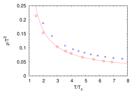
Figure 1: Thermal monopole density (circles) as function of temperature. For comparison data from Ref. D’Alessandro and D’Elia (2008) are shown (squares). The curve shows fit to eq.(6).

The dimensional reduction suggests for the density $\rho$ the following temperature dependence at high enough temperature

$$\rho(T)=(c_{\rho}g^{2}(T)T)^{3}$$ (6)

where the temperature dependent running coupling $g^{2}(T)$ is described at high temperature by the two-loop expression with the scale parameter $\Lambda_{T}$:

$$g^{-2}(T)=\frac{11}{12\pi^{2}}\ln(T/\Lambda_{T})+\frac{17}{44\pi^{2}}(\ln(2\ln(T/\Lambda_{T}))$$ (7)

In Ref. D’Alessandro and D’Elia (2008) the data for density $\rho$ were fitted to a fit function

$$\frac{A}{(\log(T/\Lambda_{eff}))^{\alpha}},$$ (8)

which is motivated by a one loop expression for $g^{2}(T)$. A good fit was obtained for $T/T_{c}>2$ with $\alpha=2$ and it was noted that $\alpha=3$, which corresponds to the one loop expression for $g^{2}(T)$ is compatible with data for $T>5\ T_{c}$.

We fit our data to function (6),(7) with fitting parameters $c_{\rho}$ and $\Lambda_{T}$. The reasonably good fit with $\chi^{2}/dof=1.4$ was obtained for $T\geq 3T_{c}$ with values for fit parameters $c_{\rho}=0.79(1)$, $T_{c}/\Lambda_{T}=2.52(6)$. Thus behaviour of the density $\rho(T)$ is well described by the fitting function motivated by dimensional reduction prediction. However, for the spatial string tension $\sigma_{s}(T)$ the parameter $\Lambda_{T}$ was found very different Bali et al. (1993): $T_{c}/\Lambda_{T}=13.16(17)$. This implies that the dimensionless ratio $\rho^{1/3}(T)/\sigma_{s}^{1/2}(T)$ is decreasing with temperature. This decreasing can be indeed seen from Figure 2 where this ratio is depicted. For $\sigma_{s}^{1/2}(T)$ we took the fitting function obtained in Bali et al. (1993):

$$\sqrt{\sigma_{s}(T)}=c_{s}g^{2}(T)T$$ (9)

with $c_{s}=0.369(14)$ and $T_{c}/\Lambda_{T}=13.16(17)$.

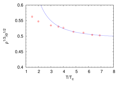
Figure 2: The ratio $\rho^{1/3}(T)/\sigma_{s}^{1/2}(T)$ as a function of temperature.

Note that decreasing seen in Figure 2 is slow, the ratio changes only about 10% over our range of temperatures. We fitted the ratio $\rho^{1/3}(T)/\sigma_{s}^{1/2}(T)$ to a polynomial fit

$$\frac{\rho^{1/3}(T)}{\sigma_{s}^{1/2}(T)}=R+R_{2}/x^{2}\,,\,\,x=T/T_{c}\,,$$ (10)

for $T/T_{c}>4$ and obtained $R=0.49(1)$. This value to be compared with respective value for $3d$ $SU(2)$. The monopole density $\rho_{3}$ in this theory was computed in Bornyakov and Grigorev (1993) : $\rho_{3}=0.0078(2)g_{3}^{6}$. Let us note that this value was obtained with the overrelaxation gauge fixing algorithm which, as is well known from $4D$ studies Bali et al. (1996), gives overestimated value for the density. Using the value for $3d$ string tension $\sigma_{3}$ from Teper (1993) $\sqrt{\sigma_{3}}=0.3353g_{3}^{2}$ we obtain for the ratio $\rho_{3}^{1/3}/\sigma_{3}^{1/2}=0.59(1)$. This is in good agreement with our value for $R$ if we take into account that the value for the $3d$ density is overestimated as was discussed above.

Thus in this section we have demonstrated that the density of monopoles changes with temperature in good agreement with predictions of the dimensional reduction and being measured in units of $\sigma_{s}^{3/2}$ is not far from its infinite temperature limit even at $T/T_{c}=1.5$.

IV Study of the interaction between monopoles.

IV.1 The details of the calculation.

In this section we study the interaction between wrapped monopoles, through the measurement of the spatial correlation function $g(r)=\langle\rho(0)\rho(r)\rangle/\rho^{2}$ for the thermal monopole-(anti)monopole pairs. On the lattice this correlation function can be measured as the ratio of the number of the (anti)monopole located at distances $(r,r+dr)$ from a given monopole and the number (anti)monopoles in the volume $4\pi r^{2}dr$ in a completely homogeneous system

$$g(r)=\frac{1}{\rho}\frac{dN(r)}{4\pi r^{2}dr},$$ (11)

where $dN(r)$ is the number of particles in a spherical shell $(r,r+dr)$, $\rho$ is the average density of monopoles. In order to take into account discretization effects we calculate the volume $4\pi r^{2}dr$ as a number of three dimensional cubes on the lattice which are located in the spherical shell $(r,r+dr)$. Note that at large distances the densities $\rho(0),\rho(r)$ become uncorrelated and $g(r)_{r\to\infty}\to 1$

We have measured the correlation functions at the following temperatures $T/T_{c}=1.5,2.0,3.0,4.8,6.9$ where our statistics was large enough. The plots of the correlation functions at temperatures $T/T_{c}=1.5,4.8$ are shown in Figure 3

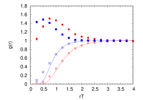
Figure 3: The correlation functions $g(r)$ for $T/T_{c}=1.5$ (squares) and 4.8 (circles) for the monopole-monopole (empty symbols) and monopole-antimonopole (full symbols) cases.

It should be noted that the plots of the correlation functions shown in Figure 3 are in agreement with the results of paper D’Alessandro and D’Elia (2008) where the same correlation functions were studied.

The correlation functions $g(r)$ contain information about interaction properties of monopoles in QGP. In order to get an idea about monopole-monopole and monopole-antimonopole interaction potentials we use the ansatz based on Boltzmann distribution

$$g(r)=\exp{\biggl{(}-\frac{U(r)}{T}\biggr{)}},$$ (12)

where $U(r)$ is the interaction potential of monopoles in QGP. Having the correlation function one can extract the interaction potential $U(r)$. The interaction potentials of monopole-(anti)monopole pairs for the lowest temperature $T/T_{c}=1.5$ and for the temperature $T/T_{c}=4.8$ are shown in Figure 4. The potentials of the monopole-(anti)monopole pairs interaction at other temperatures studied in this paper are similar to that at temperatures $T/T_{c}=1.5,4.8$.

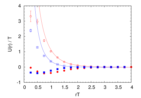
Figure 4: The potentials $U(r)$ for $T/T_{c}=1.5$ and 4.8. The symbols are the same as in Fig. 3.

IV.2 The size of monopole.

From Figure 4 it is seen that monopole-monopole repel from each other for all values of $r$. The interaction potential of monopole-antimonopole has rather complicated structure. At large distance the monopole-antimonopole attracts. However, the potential reaches minimum and after the minimum it rises, becoming repulsive.

Qualitative features of the monopole-antimonopole potential are similar to that in dilute one atomic gas. In the later case the interaction between molecules is attractive at large distances, reaches minimum at some point and becomes repulsive at distances of order of the size of molecule. From this analogue one can assume that monopoles have some size and interactions becomes repulsive at distances of order of the monopole size $r_{mon}$. In this paper we determine the size of the monopole as $2r_{mon}=r_{min}$, where $r_{min}$ is the position of the minimum of the interaction potential. In Figure 5 we plot the product $r_{mon}\sqrt{\sigma_{s}}$ as a function of temperature. Is is seen that within the error of the calculation the plot does not contradict to the behaviour which is suggested by the dimensional reduction at large temperatures. However, because of the uncertainty we cannot state that the dimensional reduction really takes place. To summarize the result of this study: monopole is not a pointlike object but an object with nontrivial core with the size $\sim 0.05-0.1$ fm depending on the temperature.

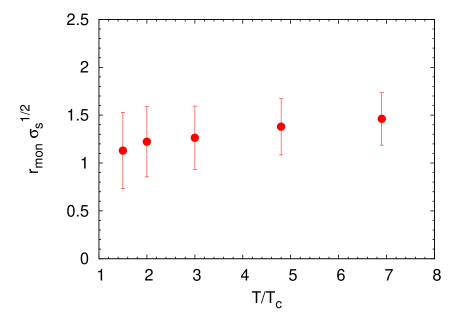
Figure 5: The product $r_{mon}\sqrt{\sigma_{s}}$ as a function of temperature.

IV.3 The tails of the correlation functions.

Now let us pay attention to the tail of the correlation functions at $r\to\infty$. In the numerical analysis we are going to fit the tail of the correlation function as it is fitted in the electromagnetic plasma

$$g(r)=\exp{\biggl{(}-\frac{\alpha}{Tr}e^{-m_{D}r}\biggr{)}},$$ (13)

where $m_{D}$ is the Debye screening mass, $\alpha$ is the monopole coupling constant. Now two comments are in order

• In electromagnetic plasma the constant $\alpha$ is the square of ion charge. However, in QGP the interaction is much more involved. In particular, the mechanism of Debye screening is not the same as it is in electromagnetic plasma. What is more important: in view of our recent finding about dyon nature of monopoles Bornyakov and Braguta (2011), one can state that monopoles interact both by chromoelectric and chromomagnetic charges. These facts mean that the constant $\alpha$ cannot be considered as a square of chromomagnetic charge.

• As was noted above correlation functions (11) are normalized as $g(r)_{r\to\infty}\to 1$. However, in lattice simulation the correlation functions at large distances differ from unity by amount $\sim 0.01$. Note the same effect was observed in paper Liao and Shuryak (2008). Analysing available data we have come to the conclusion that this is finite volume effect. In order to take into account this effect we fit our data by the function

  $$g(r)=\exp{\biggl{(}-\frac{\alpha}{Tr}e^{-m_{D}r}\biggr{)}}+c,$$ (14)

It is natural to expect that in the limit $r\to\infty$ monopole-monopole and monopole-antimonopole correlators have equal $M_{D}$ and up to the sign equal $\alpha$. Unfortunately we cannot check this since our lattices have finite sizes. It is also important that the monopole-antimonopole correlator has rather nontrivial behaviour changing from attraction to repultion at some point $r_{min}$. Evidently to get reliable estimation of the $M_{D}$ and $\alpha$ at the tail of the correlator one must consider the distances $r\gg r_{min}$ what is also impossible due to the finite lattice sizes. For this reason we determine the parameters $M_{D}$ and $\alpha$ from the monopole-monopole correlator.

In Table 2 we present the result of the fit for the monopole-monopole potential. It is seen that the fit is rather good. In Figure 6 we plot the $M_{D}/\sqrt{\sigma_{s}}$ as a function of $T/T_{c}$. From this plot one sees that within the error of the calculation the ratio $M_{D}/\sqrt{\sigma_{s}}$ does not depend on the temperature what is suggested by the dimensional reduction at large temperatures.

The authors of paper Liao and Shuryak (2008) studied the temperature dependence of the constant $\alpha$. They found that the constant $\alpha$ rises with temperature. Our results confirm the fact of rising the $\alpha$. It should also be noted that the values of the constant $\alpha$ obtained in Liao and Shuryak (2008) and in this work are a little bit different but in a reasonable agreement with each other.

The authors of paper Chernodub et al. (2004) found the value $M_{D}/\sqrt{\sigma_{s}}=1.77$. As it is seen from Figure 6 our result for this ratio is $M_{D}/\sqrt{\sigma_{s}}\simeq 2$ what is in good agreement with paper Chernodub et al. (2004), taking into the account the fact that actually the definitions of the $M_{D}$ in the both papers are different. In paper D’Alessandro and D’Elia (2008) the Debye mass was estimated $1/M_{D}\sim 0.1$ fm. Our result for the $1/M_{D}\sim 0.1-0.2$ fm depending on the temperature, what is also in reasonable agreement with the estimation of paper D’Alessandro and D’Elia (2008).

$T/T_{c}$	$M_{D}/T$	$\alpha$	$\chi^{2}/N_{dof}$
1.5	$2.2\pm 0.3$	$3.6\pm 1.3$	1.2
2.0	$1.9\pm 0.2$	$4.0\pm 1.0$	1.5
3.0	$1.7\pm 0.1$	$4.3\pm 0.5$	0.5
4.8	$1.4\pm 0.1$	$4.7\pm 0.7$	1.3
6.9	$1.4\pm 0.1$	$6.6\pm 1.5$	0.6

Table 2: The masses $M_{D}$ and coupling constants $\alpha$ obtained by fitting of the correlators to eq.(13).

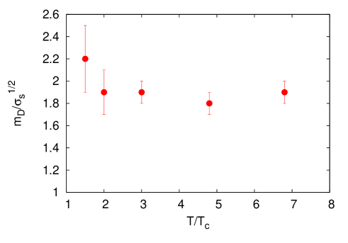
Figure 6: The ratio of $M_{D}$ to $\sqrt{\sigma_{s}}$ as a function of temperature.

V The monopole mass.

There are a lot of definitions of the monopole mass (see D’Alessandro et al. (2010)). In this paper we are going to apply the definition which is based on the formalism of functional integration. Consider the trajectory of free nonrelativistic particle of mass $m$. The spatial fluctuation of the trajectory of such particle

$$\Delta{r}^{2}=T\int_{0}^{1/T}dt\langle(\vec{r}(t)-\vec{r}(0))^{2}\rangle,$$ (15)

is directly connected to the particle mass

$$m=\frac{1}{2T\Delta{r}^{2}}.$$ (16)

The lattice version of the equation (15) can be written as

$$\Delta{r}^{2}=\frac{1}{L}\sum_{i=1}^{L}\langle(\vec{r}_{i}-\vec{r}_{1})^{2}\rangle.$$ (17)

Where the sum is taken along the monopole trajectory, $L$ is the total length of the trajectory.

With equations (16), (17) we get the result presented in Table 3. Kinetic energy of monopole is $\sim T$. Monopole mass is $\sim 2.7T$ at $T/T_{c}=1.5$ reaching $\sim 8.2T$ at $T/T_{c}=6.9$ what legitimates nonrelativistic approximation. It should be noted that the authors of paper D’Alessandro et al. (2010) also calculated the mass (16). Their result approximately $30\%$ larger than ours.

$T/T_{c}$	$a^{-2}\Delta{r}^{2}$	$m/T$
1.5	$2.97\pm 0.01$	$2.69\pm 0.01$
2.0	$2.12\pm 0.02$	$3.77\pm 0.04$
3.0	$1.53\pm 0.01$	$5.23\pm 0.03$
4.8	$1.152\pm 0.003$	$6.94\pm 0.02$
6.9	$0.975\pm 0.003$	$8.21\pm 0.03$

Table 3: The monopole masses $m$ and spatial fluctuations at different temperatures.

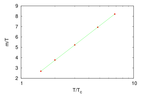
Figure 7: The monopole mass $m/T$ as a function of temperature $T/T_{c}$ in a logarithmic scale.

It should be noted that the larger the temperature the more static monopole trajectories. What means that contrary to the behaviour of the screening mass $M_{D}/T$ the monopole mass $m/T$ increases with temperature. In Fig. 7 we plot the monopole mass as a function of temperature $T/T_{c}$ in logarithmic scale. From this figure one sees that all points beautifully lie on the line

$$\frac{m}{T}=b\log{\biggl{(}\frac{T}{\Lambda_{m}}\biggr{)}},$$ (18)

with $b=3.653(6),\Lambda_{m}/T_{c}=0.718(2),~{}~{}\chi^{2}/dof\simeq 0.2$. This means that $m/T\sim 1/g^{2}(T)$ or $\Delta x^{2}T^{2}\sim g^{2}(T)$.

VI The continuum limit.

To check the continuum limit of our results we have generated 1000 configurations of lattice 8$\times$48³ with $\beta=2.635$. The temperature of these configurations is $T/T_{c}=1.5$ and it is equal to the temperature of the configurations at lattice 4$\times$36³ with $\beta=2.43$ but the lattice spacing is two times smaller.

First we note that the monopole density calculated at lattices with $a=0.1$ fm and $a=0.05$ fm differs from each other by $\sim 5\%$. What can be considered as a good continuum scaling and that even at lattice with $a=0.1$ fm we are not far from the continuum limit.

Further let us consider monopole correlators. In Fig. 8 we plot the correlators at different lattice spacings. From this plot one sees that both monopole-monopole and monopole-antimonopole correlators are in good agreement with each other at distances $rT\geq 0.7$. At distances $rT\leq 0.7$ the correlators differ from each other. However, this difference can be attributed to the fact that the lattice spacing $a=0.1$ fm is too large and the lattice to rude to probe internal monopole structure. At the same time the lattice spacing $a=0.05$ fm is small enough to do this. Note that the domain of repultion of the monopole-antimonopole pair is clearly seen on this plot.

In section IV the size of monopole was defined as $2r_{mon}=r_{0}$, where $r_{0}$ is the position of the maximum in the monopole-antimonopole correlator. The position of the maximum shifted to the right but not greater than by $20\%$. If the maximum were lattice artefact for dimensional arguments its position would shift to the left. From this we conclude that monopole has some physical size which has good scaling behaviour.

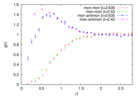
Figure 8: Monopole-monopole and monopole-antimonopole correlators at temperature $T/T_{c}=1.5$ for lattices 8$\times$48³ with $a=0.1$ fm and $\beta=2.635$ with $a=0.05$ fm.

The tail parameters $\alpha,M_{D}/T$ (14) and monopole mass $m/T$ (16) at lattice with $a=0.05$ fm have the following values

$$\alpha=3.0\pm 0.8,\quad\frac{M_{D}}{T}=1.9\pm 0.2,\quad\frac{m}{T}=3.96\pm 0.2.$$ (19)

We see that taking into the account uncertainties of the calculation the results for the $\alpha,M_{D}/T$ are in agreement with Table 2. As to the monopole mass $m/T$ its value is by $30\%$ larger than the result presented in Table 3. Note that Table 3 was obtained at lattices with $N_{t}=4$, but results Table 19 were obtained at lattice with $N_{t}=8$. Evidently, the thermal monopole trajectory parameters are very sensitive to the $N_{t}$. So, this could be the reason of the deviation of the both results.

VII Conclusion.

In this paper the properties of the thermal abelian monopoles are studied in the deconfinement phase of the $SU(2)$ gluodynamics. To remove effects of Gribov copies the simulated annealing algorithm is applied for fixing the maximally abelian gauge.

We calculated the density of thermal abelian monopoles at different temperatures. It was found that at temperatures $T>3T_{c}$ our data can be very well fitted by the function which is motivated by dimensional reduction prediction $\rho\sim(g^{2}(T)T)^{3}$.

I addition to the monopole density in this paper we studied the monopole-(anti)monopole spatial correlation functions. We calculated the correlation functions at the temperatures $T/T_{c}=1.5,2.0,3.0,4.8,6.9$. This result allowed us to determine the potentials of monopole-monopole and monopole-antimonopole interactions. As one can expect monopoles repel from each other. The tails of the interaction potential can be well fitted by the screened Coulumb potential

$$U(r)=\frac{\alpha}{r}e^{-M_{D}r}.$$ (20)

We determined the dependence of the parameters $\alpha,M_{D}$ on temperature.

The interaction potential of monopole-antimonopole has rather complicated structure. At large distances it is attractive. However, the potential has a minimum at some distance and after the minimum it rises, becoming repulsive. The position of the minimum can be considered as a double monopole size. In this way we estimated the size of monopole which turned out to be $0.05-0.1$ fm depending on the temperature.

We have also calculated the mass of monopole and the dependence of the mass on temperature.

The last point considered in this paper is the continuum limit of the results obtained in this paper. The calculation was done at lattice 8$\times$48³ with two times smaller lattice spacing $a=0.05$ fm in comparison to the lattice 4$\times$36³ (see Table 1). All results except the monopole mass have good scaling behaviour. The monopole mass is increased by 30%. To undestand the origin of this increase further study is needed.

Acknowledgments

We would like to express our gratitude to M.I. Polikarpov and V.I. Zakharov for very useful and illuminating discussions. This investigation has been supported by the Federal Special-Purpose Programme ’Cadres’ of the Russian Ministry of Science and Education, by the grant for scientific schools NSh-6260.2010.2 and by grant RFBR 11-02-01227-a. VVB is supported by grant RFBR 10-02-00061-a and RFBR 11-02-00015-a. VGB is supported by grant RFBR 09-02-00338-a.

References

- Liao and Shuryak (2007) J. Liao and E. Shuryak, Phys. Rev. C75, 054907 (2007), eprint hep-ph/0611131.
- Chernodub and Zakharov (2007) M. N. Chernodub and V. I. Zakharov, Phys. Rev. Lett. 98, 082002 (2007), eprint hep-ph/0611228.
- Shuryak (2009) E. Shuryak, Prog. Part. Nucl. Phys. 62, 48 (2009), eprint 0807.3033.
- ’t Hooft (1981) G. ’t Hooft, Nucl.Phys. B190, 455 (1981).
- ’t Hooft (1982) G. ’t Hooft, Phys.Scripta 25, 133 (1982).
- Kronfeld et al. (1987) A. S. Kronfeld, G. Schierholz, and U. Wiese, Nucl.Phys. B293, 461 (1987).
- Suzuki and Yotsuyanagi (1990) T. Suzuki and I. Yotsuyanagi, Phys.Rev. D42, 4257 (1990).
- Suzuki (1993) T. Suzuki, Nucl.Phys.Proc.Suppl. 30, 176 (1993).
- Chernodub and Polikarpov (1997) M. Chernodub and M. Polikarpov (1997), eprint hep-th/9710205.
- Ripka (2003) G. Ripka (2003), lectures delivered at European Center for Theoretical Studies in Nuclear Physics and Related Areas, 2002-2003, ECT, Trento, Italy, eprint hep-ph/0310102.
- Bornyakov et al. (1992) V. G. Bornyakov, V. K. Mitrjushkin, and M. Muller-Preussker, Phys. Lett. B284, 99 (1992).
- Ejiri (1996) S. Ejiri, Phys. Lett. B376, 163 (1996), eprint hep-lat/9510027.
- D’Alessandro and D’Elia (2008) A. D’Alessandro and M. D’Elia, Nucl. Phys. B799, 241 (2008), eprint 0711.1266.
- Bali et al. (1996) G. Bali, V. Bornyakov, M. Muller-Preussker, and K. Schilling, Phys.Rev. D54, 2863 (1996), eprint hep-lat/9603012.
- Bali et al. (1993) G. Bali, J. Fingberg, U. M. Heller, F. Karsch, and K. Schilling, Phys.Rev.Lett. 71, 3059 (1993), eprint hep-lat/9306024.
- Heller et al. (1998) U. M. Heller, F. Karsch, and J. Rank, Phys. Rev. D57, 1438 (1998), eprint hep-lat/9710033.
- Bornyakov and Grigorev (1993) V. Bornyakov and R. Grigorev, Nucl. Phys. Proc. Suppl. 30, 576 (1993).
- Teper (1993) M. Teper, Phys.Lett. B311, 223 (1993).
- Bornyakov and Braguta (2011) V. Bornyakov and V. Braguta (2011), eprint 1104.1063.
- Liao and Shuryak (2008) J. Liao and E. Shuryak, Phys.Rev.Lett. 101, 162302 (2008), eprint 0804.0255.
- Chernodub et al. (2004) M. Chernodub, K. Ishiguro, and T. Suzuki, Prog.Theor.Phys. 112, 1033 (2004), eprint hep-lat/0407040.
- D’Alessandro et al. (2010) A. D’Alessandro, M. D’Elia, and E. V. Shuryak, Phys. Rev. D81, 094501 (2010), eprint 1002.4161.