Coupling of bouncing-ball modes to the chaotic sea and their counting function

Abstract

We study the coupling of bouncing-ball modes to chaotic modes in two-dimensional billiards with two parallel boundary segments. Analytically, we predict the corresponding decay rates using the fictitious integrable system approach. Agreement with numerically determined rates is found for the stadium and the cosine billiard. We use this result to predict the asymptotic behavior of the counting function $N_{\text{bb}}(E)\sim E^{\delta}$. For the stadium billiard we find agreement with the previous result $\delta=3/4$. For the cosine billiard we derive $\delta=5/8$, which is confirmed numerically and is well below the previously predicted upper bound $\delta=9/10$.

I Introduction

Two-dimensional billiard systems have found abundant applications in contemporary physics such as for electromagnetic and acoustic resonators, microdisk lasers, atomic matter waves in optical billiards, and quantum dots Sto1999 ; NoeSto1997 ; FriKapCarDav2001 ; EllSchBer2001 ; MarRimWesHopGos1992 . The classical dynamics of these billiards is described by a point particle of mass $M$ moving with constant velocity inside a domain $\Omega$ with elastic reflections at its boundary $\partial\Omega$. Depending on the shape of the boundary the phase space can be regular, mixed regular-chaotic, or chaotic. Quantum mechanically, billiards are described by the time-independent Schrödinger equation (in units $\hbar=2M=1$)

$$-\Delta\psi_{l}(x,y)=E_{l}\psi_{l}(x,y),\quad(x,y)\in\Omega$$ (1)

with Dirichlet boundary condition $\psi_{l}=0$ on $\partial\Omega$, eigenfunctions $\psi_{l}$, eigenvalues $E_{l}$, Laplace operator $\Delta$, and $l\in\mathbb{N}$.

Many nonintegrable billiards of interest contain a rectangular region combined with other boundary segments, for example the stadium Bun1979 , the Sinai Sin1970 , and the cosine billiard Sti1996 ; see Fig. 1. Classically, in these billiards a family of marginally stable periodic orbits exists, which bounce with perpendicular reflections between the two parallel parts of the boundary. These so-called bouncing-ball orbits are surrounded by chaotic motion in phase space. For simplicity we will only consider billiards which show no visible regular regions. Quantum mechanically, most of the eigenfunctions $\psi_{l}$ are chaotic; i.e., they extend over the whole chaotic phase space. In contrast, the so-called bouncing-ball modes $\psi_{mn}$ Hel1984 ; BaiHosSteTay1985 ; OcoHel1988 ; McdKau1988 ; BogSch2004 ; BurZwo2005 concentrate on the marginally stable periodic orbits. They have a structure similar to the eigenstates of a rectangle; see Figs. 1(c) and 1(d), and are characterized by the quantum numbers $m$ and $n$, where $m$ describes the quantization along the bouncing-ball orbits and $n$ perpendicular to them. In Ref. Has2010 it was proven that semiclassically the modes with $n=1$ and increasing $m$ exist. For the counting function $N_{\text{bb}}(E)$ of the bouncing-ball modes up to energy $E$ this sequence of modes leads to $N_{\text{bb}}(E)\sim\sqrt{E}$. Typically also modes with higher excitations $n>1$ perpendicular to the periodic orbits exist for large enough $m$. Which bouncing-ball modes $\psi_{mn}$ are realized for a specific billiard depends on the couplings of the bouncing-ball modes to the chaotic modes. For fixed $m$ these couplings increase with $n$ such that for large $n$ the bouncing-ball modes couple to many neighboring chaotic modes and thus disappear. One expects that the number of bouncing-ball modes is asymptotically described by a power law $N_{\text{bb}}(E)\propto E^{\delta}$ with exponent $1/2\leq\delta<1$. The exponent $\delta=1$ cannot be achieved in ergodic billiards, as quantum ergodicity Shn1974 ; Ver1985 ; Zel1987 ; GerLei1993 ; ZelZwo1996 requires that the fraction of exceptional eigenfunctions must vanish, i.e., $N_{\text{bb}}(E)/N(E)\to 0$, where $N(E)\sim E$ is the total number of eigenstates.

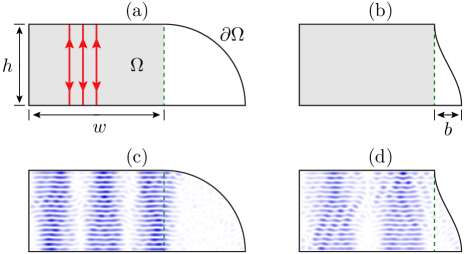
Figure 1: (Color online) Schematic pictures of the desymmetrized (a) stadium and (b) cosine billiard. Each billiard has a rectangular bouncing-ball region (gray shaded) of width $w$ and height $h$. In the rectangular region so-called bouncing-ball orbits exist perpendicular to the parallel parts of the boundary (red vertical lines). In (c) and (d) bouncing-ball modes are shown for the stadium and the cosine billiard, respectively.

The exponent $\delta$ depends on the shape of the billiard in the vicinity of the rectangular bouncing-ball region. In Ref. Tan1997 it was shown that for the stadium billiard the exponent $\delta=3/4$ arises, using an EBK-like quantization of the bouncing-ball modes. With a different approach based on an adiabatic approximation BaiHosSteTay1985 of the bouncing-ball modes an upper bound for the exponent $\delta$ was obtained for any chaotic billiard with a rectangular bouncing-ball region BaeSchSti1997 . For the stadium billiard this bound agrees with $\delta=3/4$ from Ref. Tan1997 . For the cosine billiard a bound of $\delta=9/10$ was obtained and $\delta\approx 0.87$ was observed numerically.

In this paper we relate the couplings between bouncing-ball modes and chaotic modes to the number $N_{\text{bb}}(E)$ of bouncing-ball modes in a billiard. The couplings give rise to decay rates $\gamma$, which describe the initial exponential decay $\sim$$\text{e}^{-\gamma t}$ of states concentrating on the marginally stable periodic orbits to the chaotic region of phase space. In order to predict the decay rates $\gamma$ we employ the fictitious integrable system approach BaeKetLoeSch2008 ; BaeKetLoe2010 , which was previously used to determine regular-to-chaotic tunneling rates in systems with a mixed phase space BaeKetLoeSch2008 ; BaeKetLoeRobVidHoeKuhSto2008 ; BaeKetLoeWieHen2009 ; LoeBaeKetSch2010 ; BaeKetLoe2010 . We find a power-law decrease of the decay rates with increasing energy. We argue that the decreasing $\gamma$ imply the semiclassical existence of the bouncing-ball modes, complementing previous approaches OcoHel1988 ; Tan1997 ; Has2010 . Furthermore, we use this prediction of decay rates to count the number of bouncing-ball modes $N_{\text{bb}}(E)$. For the stadium billiard we confirm the prediction of $\delta=3/4$ Tan1997 ; BaeSchSti1997 . For the cosine billiard we derive the exponent $\delta=5/8=0.625$, which is well below the previously predicted upper bound $\delta=9/10$ BaeSchSti1997 . Numerically we observe $\delta\approx 0.64$ using a larger energy range than in Ref. BaeSchSti1997 , where $\delta\approx 0.87$ was found.

This paper is organized as follows. In Sec. II we review the fictitious integrable system approach, derive a prediction for the decay rates of bouncing-ball modes, and compare the results to numerically determined rates. As examples we consider the ergodic stadium billiard and the cosine billiard at parameters, where no regular motion is visible in phase space. In Sec. III we use the prediction of decay rates to determine the number $N_{\text{bb}}(E)$ of bouncing-ball modes and compare the results to the literature Tan1997 ; BaeSchSti1997 . A summary is given in Sec. IV.

II Coupling of bouncing-ball modes

For the analysis of the coupling of bouncing-ball modes to the chaotic sea we use the analogy to systems with a mixed phase space. There the coupling of regular and chaotic modes is caused by dynamical tunneling DavHel1981 , which quantum mechanically connects the classically separated regular and chaotic regions. The billiards studied in this paper have no regular islands in phase space. However, there is a region surrounding the marginally stable bouncing-ball orbits which acts like a regular island, whose border is energy dependent such that its area semiclassically goes to zero Tan1997 . For this situation we apply the fictitious integrable system approach BaeKetLoeSch2008 ; BaeKetLoe2010 to predict the couplings of bouncing-ball modes to the chaotic sea. Whether this coupling occurs due to dynamical tunneling as in mixed systems, or due to classically allowed transitions, e.g., through partial barriers, or some other mechanism is an open question that we do not address in this paper.

II.1 The fictitious integrable system approach

We first give a brief review of the fictitious integrable system approach BaeKetLoe2010 which was previously used to determine regular-to-chaotic tunneling rates in systems with a mixed phase space BaeKetLoeSch2008 ; BaeKetLoeRobVidHoeKuhSto2008 ; BaeKetLoeWieHen2009 ; LoeBaeKetSch2010 ; BaeKetLoe2010 . Here it is applied in order to predict couplings of bouncing-ball modes in chaotic billiards. The main idea of the fictitious integrable system approach is the decomposition of Hilbert space into two parts, which correspond to the bouncing-ball modes (regular subspace) and to the remaining chaotic modes (chaotic subspace). Such a decomposition can be found by introducing a fictitious integrable system $H_{\text{reg}}$. This system has to be chosen such that its classical dynamics is integrable and contains the marginally stable bouncing-ball motion of the chaotic billiard. Quantum mechanically, the eigenstates $|\psi_{\text{reg}}^{mn}\rangle$ of $H_{\text{reg}}$, $H_{\text{reg}}|\psi_{\text{reg}}^{mn}\rangle=E_{\text{reg}}^{mn}|\psi_{\text{reg}}^{mn}\rangle$, closely resemble the bouncing-ball modes of the chaotic billiard and are used as a basis for the regular subspace. The regular modes $|\psi_{\text{reg}}^{mn}\rangle$ are characterized by two quantum numbers $m$ and $n$, where $m$ describes the quantization along the bouncing-ball orbits and $n$ perpendicular to them. They localize on quantizing tori of $H_{\text{reg}}$, and decay beyond. This decay is the decisive property of $|\psi_{\text{reg}}^{mn}\rangle$, which have no chaotic admixture, in contrast to bouncing-ball modes in a chaotic billiard. Two choices for the system $H_{\text{reg}}$ will be discussed in Sec. II.2.

Introducing a basis $|\psi_{\text{ch}}\rangle$ in the chaotic subspace, the coupling matrix element of one regular mode $|\psi_{\text{reg}}^{mn}\rangle$ and a chaotic mode $|\psi_{\text{ch}}\rangle$ is given by

$$v_{\text{ch},mn}=\langle\psi_{\text{ch}}|H|\psi_{\text{reg}}^{mn}\rangle.$$ (2)

The disadvantage of these couplings $v_{\text{ch},mn}$ is their dependence on the size of the chaotic region via the normalization of the chaotic modes $|\psi_{\text{ch}}\rangle$. A better suited quantity, that is not affected by such changes, is the decay rate $\gamma$. Under variation of the billiard boundary far away from the rectangular bouncing-ball region it is unique for each regular state $|\psi_{\text{reg}}^{mn}\rangle$. From the couplings $v_{\text{ch},mn}$ the decay rate is obtained with Fermi’s golden rule

$$\gamma_{mn}=2\pi\langle|v_{\text{ch},mn}|^{2}\rangle\rho_{\text{ch}}.$$ (3)

Here we average over the modulus squared of the fluctuating coupling matrix elements $v_{\text{ch},mn}$ of one particular regular mode and different chaotic modes of similar energy. The chaotic density of states is approximated by the leading Weyl term $\rho_{\text{ch}}\approx A/(4\pi)$, in which $A$ denotes the area of the billiard.

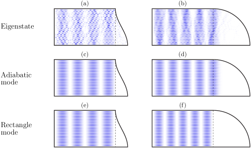
Figure 2: (Color online) Comparison of bouncing-ball modes of (a) the cosine billiard with quantum number $(23,4)$ and (b) the stadium billiard with quantum number $(23,5)$ to the corresponding adiabatic modes [(c), (d)] and to the rectangle modes [(e), (f)]. The adiabatic modes (c) and (d) closely resemble the bouncing-ball modes (a) and (b), respectively. The rectangle mode (e) closely resembles the bouncing-ball mode (a) of the cosine billiard, while for the stadium billiard the rectangle mode (f) fails to reproduce the bouncing-ball mode (b).

To illustrate the decay rates $\gamma$ one may consider a regular state $|\psi_{\text{reg}}^{mn}\rangle$ concentrating close to the marginally stable bouncing-ball orbits which is coupled to a continuum of chaotic states. Its decay $\sim$$\text{e}^{-\gamma_{mn}t}$ is characterized by the rate $\gamma_{mn}$. For systems with a finite phase space this exponential decay occurs at most up to the Heisenberg time $\tau_{H}=2\pi/\Delta$, where $\Delta$ is the mean level spacing. Alternatively, the decay rates are the inverse of the lifetimes of resonances in a corresponding open system, which can be obtained, e.g., by adding an absorbing region in the chaotic component of phase space far away from the bouncing-ball region.

II.2 Integrable approximations

In the following we predict decay rates $\gamma$ of bouncing-ball modes with Eqs. (2) and (3). For this we construct a fictitious integrable system $H_{\text{reg}}$, whose eigenstates $|\psi_{\text{reg}}^{mn}\rangle$ resemble the bouncing-ball modes of the chaotic billiard. Two approaches will be presented below. The first uses adiabatic modes, which approximate the bouncing-ball modes quite well, but have to be evaluated numerically. The second approach uses modes of the rectangular billiard, which are given analytically, but turn out to be a good approximation for the bouncing-ball modes of the cosine billiard only.

II.2.1 Adiabatic-mode approximation

In order to construct modes which approximate the bouncing-ball modes of a billiard we use the adiabatic separation ansatz BaiHosSteTay1985

$$\psi_{\text{reg}}^{mn}(x,y)=\varphi_{m}(y;x)\chi_{mn}(x)$$ (4)

with

$$\varphi_{m}(y;x)=\sqrt{\frac{2}{h(x)}}\sin\left(\frac{m\pi y}{h(x)}\right),$$ (5)

where $h(x)$ is the height of the billiard at $x$ with $h(0)=h$. Equation (4) is close to a separation ansatz but $\varphi_{m}$ weakly depends on $x$ in order to satisfy the Dirichlet boundary condition on $\partial\Omega$. The function $\varphi_{m}$ accounts for the quantization of the fast bouncing-ball motion in the $y$ direction. The slow motion in the $x$ direction is quantized by demanding that $\chi_{mn}$ fulfills the 1D Schrödinger equation BaiHosSteTay1985 ,

$$-\chi_{mn}^{{}^{\prime\prime}}(x)+m^{2}V(x)\chi_{mn}(x)=e_{mn}\chi_{mn}(x),$$ (6)

which we solve numerically. Here the effective potential is $m^{2}V(x)$ with

$$V(x)=\frac{\pi^{2}}{h(x)^{2}}-\frac{\pi^{2}}{h^{2}}$$ (7)

and the eigenvalues are denoted by $e_{mn}$. From $e_{mn}$ one obtains approximate eigenvalues of the bouncing-ball modes $E_{\text{reg}}^{mn}=m^{2}\pi^{2}/h^{2}+e_{mn}$. The ansatz, Eq. (4), exactly satisfies the Schrödinger equation inside the rectangular region of the billiard. Outside of the rectangular region this is only approximately true. There the functions $\chi_{mn}(x)$ will eventually decay exponentially, as the effective potential $m^{2}V(x)$ becomes very steep for large $m$.

The adiabatic modes show good agreement to the bouncing-ball modes of the stadium and the cosine billiard if $n\ll m$; see Figs. 2(a)-2(d). In particular the bouncing-ball modes are well reproduced in the region $x\approx w$, where the rectangular region ends. Note that small deviations arise for modes with large $n$, in particular for the stadium billiard (not shown). However, these modes strongly couple to chaotic modes and thus do not contribute to the counting function in Sec. III.

We now predict decay rates of bouncing-ball modes using the adiabatic modes $|\psi_{\text{reg}}^{mn}\rangle$. Replacing the coupling matrix elements $v_{\text{ch},mn}$ in Eq. (3) by Eq. (2) we find for the decay rates

$$\gamma_{mn} = \frac{2\pi\rho_{\text{ch}}}{N_{\Delta}}\langle\psi_{\text{reg}}^{mn}|H\left(\sum_{\text{ch},\Delta E}|\psi_{\text{ch}}\rangle\langle\psi_{\text{ch}}|\right)H|\psi_{\text{reg}}^{mn}\rangle$$ (8)

$$= \frac{2\pi\rho_{\text{ch}}}{N_{\Delta}}\|P_{\text{ch},\Delta E}H|\psi_{\text{reg}}^{mn}\rangle\|^{2}.$$ (9)

To obtain Eq. (8) we express the average in Eq. (3) by a sum over all chaotic states $|\psi_{\text{ch}}\rangle$ in an energy interval $\Delta E$ around the energy $E_{\text{reg}}^{mn}$ of the adiabatic mode and $N_{\Delta}$ is the number of chaotic states in this energy interval. The term $\sum_{\text{ch},\Delta E}|\psi_{\text{ch}}\rangle\langle\psi_{\text{ch}}|$ in Eq. (8) is equal to a projector $P_{\text{ch},\Delta E}$ onto the chaotic subspace in the considered energy interval. We approximate this projector using the adiabatic modes $|\psi_{\text{reg}}^{mn}\rangle$,

$$P_{\text{ch},\Delta E}\approx P_{\Delta E}\left(\mathds{1}-\sum_{m^{\prime}\geq n^{\prime}}|\psi_{\text{reg}}^{m^{\prime}n^{\prime}}\rangle\langle\psi_{\text{reg}}^{m^{\prime}n^{\prime}}|\right).$$ (10)

Here $P_{\Delta E}$ projects onto the energy interval $[E_{\text{reg}}^{mn}-\Delta E/2,E_{\text{reg}}^{mn}+\Delta E/2]$. The choice $m^{\prime}\geq n^{\prime}$ for the sum ensures that $P_{\text{ch},\Delta E}$ projects onto the phase-space component with $k_{x}/h\geq k_{y}/w$, which excludes the bouncing-ball region but also parts of the surrounding chaotic region. This choice will underestimate the decay rates slightly. However, a more precise projection would require an a priori knowledge of the energy-dependent border between the bouncing-ball region and the chaotic region. Using Eq. (10) in Eq. (9) the decay rates are determined by

$$\gamma_{mn}=\frac{A}{2N_{\Delta}}\left\|P_{\Delta E}H|\psi_{\text{reg}}^{mn}\rangle-\sum_{(m^{\prime},n^{\prime})\in\Delta E}v_{m^{\prime}n^{\prime},mn}|\psi_{\text{reg}}^{m^{\prime}n^{\prime}}\rangle\right\|^{2},$$ (11)

where

$$v_{m^{\prime}n^{\prime},mn}=\langle\psi_{\text{reg}}^{m^{\prime}n^{\prime}}|H|\psi_{\text{reg}}^{mn}\rangle$$ (12)

and $\rho_{\text{ch}}\approx A/(4\pi)$ has been used. In order to numerically evaluate the term $P_{\Delta E}H|\psi_{\text{reg}}^{mn}\rangle$ in Eq. (11) we expand the state $|\psi_{\text{reg}}^{mn}\rangle$ in the eigenbasis $|\psi_{l}\rangle$ of $H$ in the energy interval $[E_{\text{reg}}^{mn}-\Delta E/2,E_{\text{reg}}^{mn}+\Delta E/2]$ such that $P_{\Delta E}H|\psi_{\text{reg}}^{mn}\rangle=\sum_{\Delta E}c_{l}E_{l}|\psi_{l}\rangle$, where $c_{l}=\langle\psi_{l}|\psi_{\text{reg}}^{mn}\rangle$. With this procedure Eq. (11) can be evaluated numerically for all bouncing-ball modes of quantum number $(m,n)$. We find good agreement to numerically determined rates for the cosine and the stadium billiard; see Sec. II.3.

II.2.2 Rectangle-mode approximation

While the approach for the determination of decay rates presented in the last section is applicable for any billiard with a rectangular bouncing-ball region, an analytical result is not available. In order to find such an analytical result we now approximate the bouncing-ball modes by the eigenstates $|\psi_{\text{reg}}^{mn}\rangle$ of a rectangular billiard and construct the chaotic states $|\psi_{\text{ch}}\rangle$ entering in Eq. (2) by a random-wave model Ber1977 . As chaotic states $|\psi_{\text{ch}}\rangle$ modeled in this way are not orthogonal to the regular states $|\psi_{\text{reg}}^{mn}\rangle$, Eq. (2) has to be modified (see Sec. II A in Ref. BaeKetLoe2010 ), which leads to the approximation

$$v_{\text{ch},mn}=\langle\psi_{\text{ch}}|H-H_{\text{reg}}|\psi_{\text{reg}}^{mn}\rangle.$$ (13)

The simplest approximation of a rectangular bouncing-ball region of width $w$ and height $h$ is given by the rectangular billiard of the same width and height. We now use this billiard as the fictitious integrable system $H_{\text{reg}}$ in Eq. (13). Its eigenstates in position representation are given analytically by

$$\psi_{\text{reg}}^{mn}(x,y)=\frac{2}{\sqrt{wh}}\sin\left(\frac{n\pi x}{w}\right)\sin\left(\frac{m\pi y}{h}\right)$$ (14)

with eigenenergies $E_{\text{reg}}^{mn}=\pi^{2}m^{2}/h^{2}+\pi^{2}n^{2}/w^{2}$. Note that these rectangle modes $\psi_{\text{reg}}^{mn}(x,y)$ are zero for $x\geq w$, while the bouncing-ball modes of chaotic billiards will typically extend into this region. Hence, the rectangle modes will only be an approximation of the true eigenstates of the billiard. Figure 2 shows that the rectangle modes are good approximations for the bouncing-ball modes of the cosine billiard, which has a corner of angle $\pi/2$ at $x=w$, but not for the bouncing-ball modes of the stadium billiard, which substantially extend beyond $x=w$. As the fictitious integrable system approach relies on a good approximation of the bouncing-ball modes, the following prediction of decay rates is expected to apply only for billiards which have a corner of angle $\pi/2$ at $x=w$, like the cosine billiard.

When evaluating Eq. (13) an infinite potential difference arises between the Hamiltonian $H$ of the chaotic billiard and $H_{\text{reg}}$ of the rectangle, $H-H_{\text{reg}}=-\infty$, for $x\geq w$. At the same time for the rectangle modes $\psi_{\text{reg}}^{mn}(x,y)=0$ holds in that region, which leads to an undefined product $-\infty\cdot 0$. Similar to the approach presented for the mushroom billiard in Refs. BaeKetLoeRobVidHoeKuhSto2008 ; BaeKetLoe2010 we circumvent this problem by introducing a rectangular billiard which is extended by a finite potential $W$ at $x\geq w$ for which in the end the limit $W\to\infty$ is taken. This leads to

$$v_{\text{ch},mn}=\int\limits_{0}^{h}\text{d}y\,\psi_{\text{ch}}(x=w,y)\,\partial_{x}\psi_{\text{reg}}^{mn}(x=w,y).$$ (15)

For completeness we now give the derivation of Eq. (15) following Refs. BaeKetLoeRobVidHoeKuhSto2008 ; BaeKetLoe2010 : We first introduce a rectangular billiard which is extended by a finite potential $W$ for $x\geq w$,

$$H_{\text{reg}}^{W} = p_{x}^{2}+p_{y}^{2}+V(x,y)$$ (16)

$$V(x,y) = \left\{\begin{array}[]{ll}0&\quad\text{for }0<x<w,\;0<y<h\\ W&\quad\text{for }x\geq w,\;0<y<h\\ \infty&\quad\text{otherwise}\end{array}\right.$$ (20)

and consider the limit $W\to\infty$ in which the original rectangular billiard is recovered. For finite $W$ the regular eigenfunctions $\psi_{\text{reg},W}^{mn}(x,y)$ of $H_{\text{reg}}^{W}$ decay into the region $x\geq w$, which is described by

$$\psi_{\text{reg},W}^{mn}(x,y)=\psi_{\text{reg},W}^{mn}(x=w,y)\text{e}^{-\lambda(x-w)}.$$ (21)

Here $\lambda$ depends on $W$ via the Schrödinger equation as

$$-\lambda^{2}+W=E_{mn}^{W}.$$ (22)

Since the derivative of the regular eigenfunctions $\psi_{\text{reg},W}^{mn}$ has to be continuous at $x=w$ we obtain

$$\partial_{x}\psi_{\text{reg},W}^{mn}(x=w,y)=-\lambda\,\psi_{\text{reg},W}^{mn}(x=w,y).$$ (23)

This can be used for rewriting Eq. (13) for the coupling matrix elements

$$v_{\text{ch},mn} = \lim_{W\to\infty}\int\limits_{w}^{w+b}\text{d}x\int\limits_{0}^{h(x)}\text{d}y\,\psi_{\text{ch}}(x,y)(-W)\psi_{\text{reg},W}^{mn}(x,y)\quad\;\;$$ (24)

$$= \lim_{W\to\infty}\int\limits_{w}^{w+b}\text{d}x\int\limits_{0}^{h(x)}\text{d}y\,\psi_{\text{ch}}(x,y)\frac{W}{\lambda}\text{e}^{-\lambda(x-w)}\partial_{x}\psi_{\text{reg},W}^{mn}(w,y).$$ (25)

The term

$$\frac{W}{\lambda}\text{e}^{-\lambda(x-w)}=\frac{W}{\sqrt{W-E_{mn}^{W}}}\text{e}^{-\sqrt{W-E_{mn}^{W}}(x-w)}$$ (26)

reduces in the limit $W\to\infty$ to $2\delta(x-w)$ for $x\geq w$, where we used Eq. (22) and that $E_{mn}^{W}$ remains bounded. This finally leads to Eq. (15).

Evaluating the coupling matrix elements, Eq. (15), for the rectangle modes, Eq. (14), gives

$$v_{\text{ch},mn}=(-1)^{n}\frac{2}{\sqrt{wh}}\frac{n\pi}{w}\int\limits_{0}^{h}\text{d}y\,\psi_{\text{ch}}(x=w,y)\,\sin\left(\frac{m\pi y}{h}\right).$$ (27)

Therefore the decay rates $\gamma_{mn}$, Eq. (3), scale with $n^{2}$.

In order to find the scaling of the decay rates with $m$ we employ a random-wave model Ber1977 for the chaotic states $\psi_{\text{ch}}(x,y)$ entering in Eq. (27). Here it is given by

$$\psi_{\text{ch}}(x,y)=\frac{2}{\sqrt{A}}\sum_{s=1}^{s_{\text{max}}}c_{s}\sin\left(\frac{s\pi y}{h}\right)\sin(k_{x,s}x+\varphi_{s})\;\;$$ (28)

and accounts for the Dirichlet boundary conditions at $y=0$ and $y=h$, but ignores the corner at $x=w$. Here the $c_{s}$ are Gaussian-distributed random variables with mean zero and variance $\sigma_{s}=\langle c_{s}^{2}\rangle$. The phases $\varphi_{s}$ are uniformly distributed in $[0,2\pi)$, $k_{x,s}=\sqrt{E_{\text{reg}}^{mn}-\pi^{2}s^{2}/h^{2}}$, and $s_{\text{max}}=\lfloor(h/\pi)\sqrt{E_{\text{reg}}^{mn}}\rfloor$. Furthermore we define $k_{y,s}=\pi s/h$ and the angles $\alpha_{s}=\arctan(k_{y,s}/k_{x,s})$. These angles are not equidistributed on $[0,\pi/2]$; see Fig. 3. To approximate an equidistribution of directions we compensate this by appropriate weights $\sigma_{s}$, with $\sum_{s=1}^{s_{\text{max}}}\sigma_{s}=1$. A natural choice is given by assigning to each $\sigma_{s}$ half of the size of the adjacent angular intervals

$$\sigma_{s}=\frac{1}{\pi/2}\left\{\begin{array}[]{ll}(\alpha_{s+1}-\alpha_{s-1})/2\;,&1<s<s_{\text{max}}\\ \pi/2-(\alpha_{s_{\text{max}}}+\alpha_{s_{\text{max}}-1})/2\;,&s=s_{\text{max}}\\ (\alpha_{1}+\alpha_{2})/2\;,&s=1,\end{array}\right.$$ (29)

see Fig. 3.

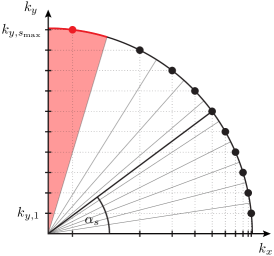
Figure 3: (Color online) Illustration of the discrete directions contributing to the random-wave model, Eq. (28), in $k$ space at energy $E_{\text{reg}}^{mn}$ (black quarter circle) with $m=10$ and $n=2$. While the wave numbers $k_{y,s}$ are equispaced, the wave numbers $k_{x,s}$ as well as the angles $\alpha_{s}$ are not equispaced. The angular regions around each $\alpha_{s}$ are marked by gray lines and the one for $\alpha_{s_{\text{max}}}$ is shaded.

Using Eq. (28) in Eq. (27) the $y$ integration over the two sine functions gives $\delta_{sm}h/2$ such that

$$v_{\text{ch},mn}=(-1)^{n}\frac{2}{\sqrt{wh}}\frac{n\pi}{w}\frac{h}{\sqrt{A}}c_{m}\sin(k_{x,m}w+\varphi_{m}).\;\;\;$$ (30)

We now determine the decay rates with Eq. (3) using an ensemble average of the modulus squared of the coupling matrix elements given by Eq. (30). This results in

$$\gamma_{mn}=\frac{\pi^{2}h}{w^{3}}n^{2}\sigma_{m}$$ (31)

which contains the weight $\sigma_{m}$. In order to find the weight $\sigma_{m}$ from Eq. (29) we have to evaluate $s_{\text{max}}$. One finds $s_{\text{max}}=m$ for small enough $n<\sqrt{2(m+1/2)}l/h$ following from $(h/\pi)\sqrt{E_{\text{reg}}^{mn}}<m+1$. We now perform a first-order expansion of the angles $\alpha_{m}$ in Eq. (29) for large $m$ and restrict to even smaller $n\ll\sqrt{m}$. We obtain

$$\sigma_{m}\approx\frac{\sqrt{2}}{\pi}\frac{1}{\sqrt{m}}$$ (32)

leading to our final result

$$\gamma_{mn}=\frac{\sqrt{2}\pi h}{w^{3}}\frac{n^{2}}{\sqrt{m}},$$ (33)

which predicts the decay rates of bouncing-ball modes characterized by the quantum numbers $m$ and $n$ to the chaotic sea for $n\ll\sqrt{m}$. For increasing $m$ the decay rates decrease like a square root while for increasing $n$ they increase quadratically.

The power-law decrease of the decay rates for constant $n$ and increasing $m$ is in contrast to the exponential decrease found for direct regular-to-chaotic tunneling rates in mixed systems, as in the mushroom billiard BarBet2007 ; BaeKetLoeRobVidHoeKuhSto2008 and in quantum maps HanOttAnt1984 ; PodNar2003 ; SheFisGuaReb2006 ; BaeKetLoeSch2008 . The decreasing decay rates for fixed $n$ lead to decreasing couplings $v_{\text{ch},mn}$, see Eq. (3), between the bouncing-ball modes and chaotic modes compared to the mean level spacing $\Delta$. This implies for large enough $m$ the semiclassical existence of the bouncing-ball mode $(m,n)$. Note that the prediction, Eq. (33), only depends on the rectangular bouncing-ball region but not on the other regions of the considered billiard. Hence, it is the same for each billiard studied in this paper. However, it can only be applied if the rectangle modes closely resemble the bouncing-ball modes. This is the case for the cosine billiard but not for the stadium billiard; see Sec. II.3 for the comparison of Eq. (33) to numerically determined rates.

II.3 Applications

We now evaluate Eqs. (11) and (33) for the decay rates of bouncing-ball modes, as discussed in Sec. II.2, and compare the results to numerically determined decay rates for specific example systems. We choose the desymmetrized cosine billiard with $w=1$, $h=0.6$, $b=0.2$, $h(x)=h\arccos(2(x-w)/b-1)/\pi$ for $x>w$, and label this billiard by $\mathcal{B}_{c}$. Furthermore we consider the desymmetrized stadium billiard with $w=1$, $h=0.6$, $h(x)=\sqrt{h^{2}-(x-w)^{2}}$ for $x>w$, and label this billiard by $\mathcal{B}_{s}$.

For the evaluation of Eq. (11) the energy interval $\Delta E$ has to be specified. We choose $\Delta E\approx 100\Delta$ with mean level spacing $\Delta$. Note that for small energy intervals $\Delta E<20\Delta$ the results of Eq. (11) show strong fluctuations, as the adiabatic states cannot be properly expanded in the eigenbasis of $H$. For $\Delta E>20\Delta$, however, the results show only small changes.

In order to calculate decay rates numerically we determine the spectrum of the stadium and the cosine billiard, using the improved method of particular solutions BetTre2005 , under variation of parts of the billiard boundary: For the cosine billiard we vary the width of the cosine part $b$ around $b=0.2$ and for the stadium we vary $w$ around $w=1$. For small variations of these parameters the eigenvalues of the bouncing-ball modes remain almost unaffected while the eigenvalues of the chaotic states show strong variations, due to the changing density of chaotic states. Analyzing up to $30$ avoided crossings $\Delta E_{\text{ch},mn}=2v_{\text{ch},mn}$ of a given bouncing-ball mode $\psi_{mn}$ with chaotic states we deduce the decay rate from Fermi’s golden rule BaeKetLoeRobVidHoeKuhSto2008 ; BaeKetLoe2010 ,

$$\gamma_{mn}=\frac{1}{8}\langle|\Delta E_{\text{ch},mn}|^{2}A\rangle.$$ (34)

Here we average over all numerically determined widths $\Delta E_{\text{ch},mn}$ and the corresponding billiard areas $A$.

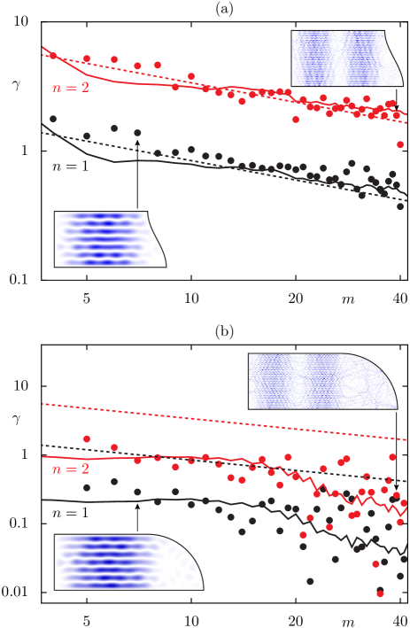
Figure 4: (Color online) Decay rates of bouncing-ball modes for (a) the cosine billiard $\mathcal{B}_{c}$ and (b) the stadium billiard $\mathcal{B}_{s}$. For the quantum numbers $n=1,2$ and increasing $m$ we compare numerical rates (dots) to the results of Eqs. (11) (solid lines) and (33) (dashed lines) on a double-logarithmic scale. The insets in (a) and (b) show the bouncing-ball modes of quantum number $(7,1)$ and $(39,2)$.

In Fig. 4(a) we show for the cosine billiard $\mathcal{B}_{c}$ numerical rates (dots) compared with the prediction of Eq. (11), using the adiabatic modes (solid lines), and Eq. (33), using the rectangle modes (dashed lines). We consider bouncing-ball modes with horizontal quantum number $n=1,2$ and increasing vertical quantum number $m$. We find very good agreement with deviations smaller than a factor of two for both predictions. The numerical rates and the results of Eq. (11) follow the power law $\gamma\sim m^{-1/2}$ predicted by Eq. (33). This confirms that for the cosine billiard the adiabatic modes as well as the rectangle modes sufficiently well approximate the bouncing-ball modes, as seen in Figs. 2(a), 2(c), and 2(e). Note that also for the desymmetrized Sinai billiard Sin1970 both predictions agree with numerical rates (not shown). It also has a corner of angle $\pi/2$ at $x=w$, such that the rectangle and the adiabatic modes closely resemble its bouncing-ball modes.

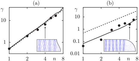
Figure 5: (Color online) Decay rates of bouncing-ball modes for (a) the cosine billiard $\mathcal{B}_{c}$ and (b) the stadium billiard $\mathcal{B}_{s}$. For the quantum numbers $m=30$ and $n=1,2,\dots$, we compare numerical rates (dots) to the results of Eqs. (11) (solid lines) and (33) (dashed lines) on a double-logarithmic scale. The insets show the bouncing-ball modes of quantum number (a) $(30,4)$ and (b) $(30,6)$.

Figure 4(b) shows the decay rates for the stadium billiard $\mathcal{B}_{s}$ for $n=1,2$ and increasing $m$. We compare the numerical rates (dots) to the prediction of Eq. (11) (solid lines), and Eq. (33) (dashed lines). Here, the average behavior of the fluctuating numerical rates agrees with the prediction of Eq. (11). As for the cosine billiard this prediction seems to follow a power-law for large $m$, however, with an exponent smaller than $-1/2$, close to $-1$. As expected, Eq. (33), based on the rectangle modes, does not reproduce the numerical rates, showing deviations by a factor of $10$. These deviations arise as the rectangle modes do not agree well enough with the bouncing-ball modes of the stadium billiard, in contrast to the adiabatic modes used in Eq. (11); see Figs. 2(b), 2(d), and 2(f). Note that the small fluctuations in the prediction arise due to the numerical evaluation of Eq. (11) and might be related to the chosen projector $P_{\text{ch},\Delta E}$. The large fluctuations in the numerically determined rates could be caused by additional couplings of the bouncing-ball modes to scars concentrating on unstable periodic orbits, which is left for future studies.

In Fig. 5 we show numerically determined decay rates and the two predictions, Eqs. (11) and (33), for bouncing-ball modes with fixed quantum number $m=30$ and increasing $n$. For both the cosine and the stadium billiard we find good agreement between the numerical rates and Eq. (11) using the adiabatic modes. Equation (33), based on the rectangle modes, is valid only for the cosine billiard as discussed before. For increasing $n$ the decay rates increase almost quadratically, $\gamma\sim n^{2}$, for both of the billiards, as found in Eq. (33).

III Counting bouncing-ball modes

We now study and predict the number of bouncing-ball modes $N_{\text{bb}}(E)$ up to energy $E$ for a billiard with a rectangular region. Due to the quantum ergodicity theorem Shn1974 in an ergodic billiard the ratio of $N_{\text{bb}}(E)$ to the total number of eigenstates $N(E)$ goes to zero in the semiclassical limit, $N_{\text{bb}}(E)/N(E)\to 0$. In addition the number of bouncing-ball modes should increase at least as $\sqrt{E}$, which gives the number of states concentrating on a one-dimensional line. Hence, one expects for the number of bouncing-ball modes

$$N_{\text{bb}}(E)=\alpha\cdot E^{\delta}+\dots\;$$ (35)

with exponent $1/2\leq\delta<1$ and prefactor $\alpha$. Here we neglect higher order terms which contain powers of the energy smaller than $\delta$.

Note that in Ref. BaeKetLoeSch2011 the boundary contribution $\sim$$\sqrt{E}$ of Eq. (35) has been determined for subsets of eigenstates in billiards. For the bouncing-ball modes in the billiards considered in this paper this boundary contribution suggests the additional term $-h/(4\pi)\sqrt{E}$. As we are not dealing with a regular region around a fixed point but an energy dependent region around the line of marginally stable bouncing-ball orbits, we expect the boundary contribution $-2h/(4\pi)\sqrt{E}$. However, it will not be considered in the following, as we are interested in the leading term only.

III.1 Counting using overlap with adiabatic modes

First we count the number of bouncing-ball modes $N_{\text{bb}}(E)$ in the cosine and the stadium billiard numerically. For this purpose we calculate their first $\approx$$3000$ eigenstates $|\psi_{l}\rangle$ and eigenvalues $E_{l}$ using the improved method of particular solutions BetTre2005 . We then determine the overlap

$$W=|\langle\psi_{l}|\psi_{\text{reg}}^{mn}\rangle|^{2}$$ (36)

of each eigenstate $|\psi_{l}\rangle$ with the adiabatic approximations $|\psi_{\text{reg}}^{mn}\rangle$ of the bouncing-ball modes. If $|\psi_{l}\rangle$ has an overlap $W>1/2$ with an adiabatic mode with $m\geq n$ we consider $|\psi_{l}\rangle$ as a bouncing-ball mode of the system. Counting the number of these modes gives a numerical estimate of $N_{\text{bb}}(E)$.

In Figs. 6(a) and 6(b) the results (black staircase functions) for the cosine and the stadium billiard are shown, respectively, on a double-logarithmic scale. For large energies the data follow in both cases a power law for the number of bouncing-ball modes, as expected from Eq. (35). Note that varying the cut off $W=1/2$ in $[0.5,0.6]$ changes the prefactors $\alpha$ but not the exponents $\delta$ (not shown).

Specifically for the stadium billiard one expects $\delta=3/4$ Tan1997 ; BaeSchSti1997 . In Fig. 6(b) we show the function $N_{\text{bb}}(E)=0.13\cdot E^{3/4}$ (red dashed line), which on a double-logarithmic scale has the same slope as the numerical data. In the inset we fit an exponent $\delta\approx 0.73$ to the data which is close to $\delta=3/4$.

For the cosine billiard $\delta=9/10$ was obtained as an upper bound and $\delta\approx 0.87$ was observed numerically BaeSchSti1997 . However, in Fig. 6(a) the data are best fitted by an exponent $\delta\approx 0.64$ (red dashed line in the inset). In order to resolve this contradiction we also studied the cosine billiard used in Ref. BaeSchSti1997 with parameters $h=1$, $w=2$, and $b=1$ (not shown). In Ref. BaeSchSti1997 numerical data for $N_{\text{bb}}(E)$ is presented which is well described by $N_{\text{bb}}(E)=\alpha E^{\delta}+\beta$ with an exponent $\delta\approx 0.87$ and a constant offset $\beta$. For the identification of the bouncing-ball modes a visual selection is performed and states up to energy $E=8400$ are considered. If we use the overlap criterion with $W>1/2$ for this cosine billiard and consider states up to energy $E=20000$ we obtain an exponent $\delta\approx 0.64$. Also a visual selection over this larger energy range gives an exponent $\delta\approx 0.7$. Hence, we conclude that the smaller energy interval used in Ref. BaeSchSti1997 is not sufficient to find the asymptotic scaling exponent.

III.2 Counting using decay rates

In Refs. BaeKetMon2005 ; BaeKetMon2007 the criterion $\gamma_{mn}<1/\tau_{H}$ has been found to describe the existence of regular states for systems with a mixed phase space. It compares the decay rates $\gamma_{mn}$ to the Heisenberg time $\tau_{H}=h/\Delta=2\pi/\Delta$. Here we apply a similar criterion to predict the number of bouncing-ball modes in a billiard, using the results (11) and (33) for the decay rates derived in Sec. II.

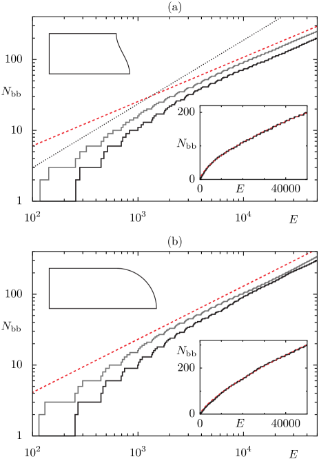
Figure 6: (Color online) Number of bouncing-ball modes $N_{\text{bb}}(E)$ for (a) the cosine billiard $\mathcal{B}_{c}$ and (b) the stadium billiard $\mathcal{B}_{s}$. We compare the results using the overlap criterion (black staircase functions) and the prediction using the decay rates (gray staircase functions) to power laws with exponent (a) $\delta=5/8$ and (b) $\delta=3/4$ (red dashed lines) on a double-logarithmic scale. In (a) we show in addition a power law with exponent $\delta=9/10$ (dotted line) BaeSchSti1997 . The insets show the results using the overlap criterion on a linear scale compared to Eq. (35) fitted for $E>10000$ (red dashed lines). We find $\delta=0.64$, $\alpha=0.196$ in (a) and $\delta=0.73$, $\alpha=0.112$ in (b).

From Eq. (3) we obtain the average coupling $\bar{v}_{mn}$ of a bouncing-ball mode to the chaotic sea,

$$\bar{v}_{mn}=\sqrt{\frac{\gamma_{mn}}{2\pi\rho_{\text{ch}}}}.$$ (37)

If this coupling $\bar{v}_{mn}$ is much smaller than $\Delta$, on average the bouncing-ball mode weakly couples to the chaotic modes such that it is visible. If the coupling is much larger than $\Delta$, on average the bouncing-ball mode couples strongly to many chaotic modes such that it is not visible. In between these two limiting cases there is a smooth transition, which was studied in Ref. BaeKetMon2007 for systems with a mixed phase space. In order to count the number of bouncing-ball modes we approximate this smooth transition by a sharp condition. The criterion $\gamma_{mn}<1/\tau_{H}$ would lead to the condition $\bar{v}_{mn}<\Delta/(2\pi)$. It is very strict in the sense that it only allows for very small couplings between the bouncing-ball modes and the chaotic modes. Approximately in the middle of the transition we find the condition

$$\bar{v}_{mn}<\frac{\Delta}{2}$$ (38)

which we use in the following for counting the number of bouncing-ball modes.

We now calculate the average coupling $\bar{v}_{mn}$ for all bouncing-ball modes up to energy $E$ with Eq. (37), using the decay rates $\gamma_{mn}$ from Eq. (11). We then count the number of those modes which fulfill the condition (38). The results are shown in Fig. 6(a) for the cosine billiard and in Fig. 6(b) for the stadium billiard as gray staircase functions. For the stadium billiard we obtain the exponent $\delta\approx 0.76$ close to $\delta=3/4$ Tan1997 ; BaeSchSti1997 and for the cosine billiard we find $\delta\approx 0.63$. Note that changing the condition (38) to $\bar{v}_{mn}<\Delta/(2\pi)$ changes the prefactor $\alpha$ but not the exponent $\delta$ for the examples we considered (not shown).

In order to obtain an analytical prediction of $N_{\text{bb}}(E)$ for the cosine billiard we use the result for the decay rates $\gamma_{mn}$, Eq. (33). Together with Eq. (37), condition (38) is fulfilled by all bouncing-ball modes with

$$n<\sqrt{\frac{\pi\Delta}{2}}\sqrt{\frac{w^{3}}{\sqrt{2}\pi h}}m^{\frac{1}{4}}.$$ (39)

For large $m$ this complies with the restriction $n\ll\sqrt{m}$ used in the derivation of Eq. (33). For the determination of $N_{\text{bb}}(E)$ one now has to count all states of quantum number $(m,n)$ for which Eq. (39) is fulfilled and $E_{\text{reg}}^{mn}=\pi^{2}m^{2}/h^{2}+\pi^{2}n^{2}/w^{2}<E$. This sum can be approximated by an integral, where we integrate the right-hand side of Eq. (39) over $m$ in the interval $[0,m_{\text{max}}]$ and approximate $m_{\text{max}}\approx\sqrt{E}h/\pi$. This finally gives for the number of bouncing-ball modes

$$N_{\text{bb}}(E)\approx\alpha\cdot E^{\frac{5}{8}}.$$ (40)

with the constant $\alpha=4w^{3/2}h^{3/4}\sqrt{\pi\Delta/2}/(5\cdot 2^{1/4}\pi^{7/4})$. Equation (40) gives the exponent $\delta=5/8$ [red dashed line in Fig. 6(a)]. It is close to the exponents $\delta\approx 0.64$ and $\delta\approx 0.63$ which were obtained using the overlap criterion and the decay rates from Eq. (11), respectively. Even the prefactor $\alpha\approx 0.34$ agrees roughly with the fitted value $\alpha\approx 0.2$. Note that Eq. (40) is only valid for billiards with a confining corner at $x=w$, as in the cosine billiard, because otherwise Eq. (33) for the decay rates cannot be applied, as in the case of the stadium billiard.

IV Summary

In this paper we study the couplings of bouncing-ball modes to chaotic modes in two-dimensional billiards and use these couplings to count the number of bouncing-ball modes. In Sec. II we apply the fictitious integrable system approach BaeKetLoeSch2008 ; BaeKetLoe2010 to predict decay rates $\gamma_{mn}$, which describe the initial decay of bouncing-ball modes into the chaotic sea. Using the adiabatic modes as approximate bouncing-ball modes we evaluate Eq. (11) and find agreement to numerical rates for the cosine and the stadium billiard. For the cosine billiard, which has a corner of angle $\pi/2$ at $x=w$, we evaluate the fictitious integrable system approach analytically using the eigenstates of the rectangular billiard as approximate bouncing-ball modes. This leads to Eq. (33) which shows excellent agreement with numerical rates. As a result we find that the decay rates of bouncing-ball modes of constant quantum number $n$ decrease as a power law with increasing energy.

In Sec. III we use the results on the decay rates in order to count the number of bouncing-ball modes $N_{\text{bb}}(E)\sim E^{\delta}$ up to energy $E$. For the stadium billiard we recover the exponent $\delta=3/4$ Tan1997 ; BaeSchSti1997 . For the cosine billiard we find $\delta\approx 0.64$. Using the analytical result Eq. (33) for the decay rates we derive $\delta=5/8$, which is in agreement with our numerics and well below the previously predicted upper bound $\delta=9/10$.

- (1) H.-J. Stöckmann, Quantum Chaos. An introduction (University Press, Cambridge, 1999).
- (2) J. U. Noeckel and A. D. Stone, Nature 385, 45 (1997).
- (3) N. Friedman, A. Kaplan, D. Carasso, and N. Davidson, Phys. Rev. Lett. 86, 1518 (2001).
- (4) C. Ellegaard, L. Schaadt, and P. Bertelsen, Physica Skripta T90, 223 (2001).
- (5) C. M. Marcus, A. J. Rimberg, R. M. Westervelt, P. F. Hopkins, and A. C. Gossard, Phys. Rev. Lett. 69, 506 (1992).
- (6) L. A. Bunimovich, Commun. Math. Phys. 65, 295 (1979).
- (7) Y. G. Sinai, Russ. Math. Surveys 25, 137 (1970).
- (8) P. Stifter, Ph.D. thesis, Universität Ulm (1996).
- (9) E. J. Heller, Phys. Rev. Lett. 53, 1515 (1984).
- (10) Y. Y. Bai, G. Hose, K. Stefański, and H. S. Taylor, Phys. Rev. A 31, 2821 (1985).
- (11) P. W. O’Connor and E. J. Heller, Phys. Rev. Lett. 61, 2288 (1988).
- (12) S. W. McDonald and A. N. Kaufman, Phys. Rev. A 37, 3067 (1988).
- (13) E. Bogomolny and C. Schmit, Phys. Rev. Lett. 92, 244102 (2004).
- (14) N. Burq and M. Zworski, SIAM Rev. 47, 43 (2005).
- (15) A. Hassel, Ann. Math. 171, 605 (2010).
- (16) A. I. Shnirelman, Usp. Mat. Nauk 29, 181 (1974).
- (17) Y. Colin de Verdière, Commun. Math. Phys. 102, 497 (1985).
- (18) S. Zelditch, Duke. Math. J. 55, 919 (1987).
- (19) P. Gérard and E. Leichtnam, Duke. Math. J. 71, 559 (1987).
- (20) S. Zelditch and M. Zworski, Comm. Math. Phys. 175, 673 (1996).
- (21) G. Tanner, J. Phys. A 30, 2863 (1997).
- (22) A. Bäcker, R. Schubert, and P. Stifter, J. Phys. A 30, 6783 (1997).
- (23) A. Bäcker, R. Ketzmerick, S. Löck, and L. Schilling, Phys. Rev. Lett. 100, 104101 (2008).
- (24) A. Bäcker, R. Ketzmerick, and S. Löck, Phys. Rev. E 82, 056208 (2010).
- (25) A. Bäcker, R. Ketzmerick, S. Löck, M. Robnik, G. Vidmar, R. Höhmann, U. Kuhl, and H.-J. Stöckmann, Phys. Rev. Lett. 100, 174103 (2008).
- (26) A. Bäcker, R. Ketzmerick, S. Löck, J. Wiersig, and M. Hentschel, Phys. Rev. A 79, 063804 (2009).
- (27) S. Löck, A. Bäcker, R. Ketzmerick, and P. Schlagheck, Phys. Rev. Lett. 104, 114101 (2010).
- (28) M. J. Davis and E. J. Heller, J. Chem. Phys. 75, 246 (1981).
- (29) M. V. Berry, J. Phys. A 10, 2083 (1977).
- (30) A. H. Barnett and T. Betcke, Chaos 17, 043125 (2007).
- (31) J. D. Hanson, E. Ott, and T. M. Antonsen, Phys. Rev. A 29, 819 (1984).
- (32) V. A. Podolskiy and E. E. Narimanov, Phys. Rev. Lett. 91, 263601 (2003).
- (33) M. Sheinman, S. Fishman, I. Guarneri, and L. Rebuzzini, Phys. Rev. A 73, 052110 (2006).
- (34) T. Betcke and L. N. Trefethen, SIAM Rev. 47, 469 (2005).
- (35) A. Bäcker, R. Ketzmerick, S. Löck, and H. Schanz, Europhys. Lett. 94, 30004 (2011).
- (36) A. Bäcker, R. Ketzmerick, and A. G. Monastra, Phys. Rev. Lett. 94, 054102 (2005).
- (37) A. Bäcker, R. Ketzmerick, and A. G. Monastra, Phys. Rev. E 75, 066204 (2007).