Joint Channel-Network Coding Strategies for Networks with Low Complexity Relays

Abstract

We investigate joint network and channel coding schemes for networks when relay nodes are not capable of performing channel coding operations. Rather, channel encoding is performed at the source node while channel decoding is done only at the destination nodes. We examine three different decoding strategies: independent network-then-channel decoding, serial network and channel decoding, and joint network and channel decoding. Furthermore, we describe how to implement such joint network and channel decoding using iteratively decodable error correction codes. Using simple networks as a model, we derive achievable rate regions and use simulations to demonstrate the effectiveness of the three decoders.

I Introduction

Classically, communication over a network involves network nodes whose sole function is the routing of packets. Recently, however, Ahlswelde et al. [1] observed that by allowing the intermediate network nodes to combine information, a greater network throughput can be obtained. This strategy is referred to as network coding.

In much of the literature on network coding, each link is assumed to have its own independent channel coding system and hence each link is assumed to be error-free. Indeed, for certain independent memoryless networks, separating the channel and network coding in this way guarantees asymptotically optimal error correction [2, 3]. However, for other networks, examples have been given showing that, in general, network and channel coding must be performed jointly to achieve the best performance [4].

Several authors have investigated this form of combining channel and network coding for the wireless relay channel. Use of iteratively decodable codes such as turbo codes [5], [6] and low-density parity-check (LDPC) codes [7], [8], [9], [10], [11] are also common. A common feature in all of these schemes is that the relay node decodes each packet prior to performing network coding. In addition, [6] and [12] include automatic repeat requests (ARQ) as another layer of error protection.

Recently, [13] and [14] have investigated networks where the network nodes have differing capabilities. In particular, [14] considers a hierarchical network where sensors have limited computing and communication capabilities and intermediate relay nodes, which communicate to a central server or access point, are more capable. On the other hand, [13] looks to minimize the capabilities required by network nodes, proposing networks where not all nodes necessarily perform coding functions.

In this paper we investigate the combination of channel and network coding in a simple cooperative network with noisy network links. Similar in spirit to [13] and [14], we assume the intermediate nodes have limited computing capabilities. In particular, we assume the intermediate nodes do not perform channel coding operations. Rather the nodes simply forward packets or perform the operation of XOR’ing two incoming packets. This differs from the traditional network coding strategy of decoding each packet at each node, XOR’ing the messages and then re-encoding the result. In our networks we only perform end-to-end channel coding, all channel encoding operations are performed at the source and all decoding operations are done at the destination. We model each link in the network as a binary symmetric channel as we assume each node makes a hard decision on its received signals.

We investigate three decoding strategies: independent network-then-channel decoding, serial network and channel decoding, and joint network and channel decoding and illustrate these strategies using LDPC codes. LDPC codes have been proposed for many network based applications including relay-networks [7], [15] and sensor networks [16]. Note that, unlike the schemes in [7] and [15], the messages in our networks are only encoded by the channel code once at the source(s) and decoded once at the destination node. Unlike the schemes in [16] the sources are not correlated.

In Section II we describe the three above-mentioned decoding strategies. In Section III we derive achievable rate regions for each decoding strategy on a simple network to demonstrate the advantage of joint decoding for cooperative networks with noisy network links and end-to-end channel coding. In Section IV we describe how iterative decoders for low-density parity-check (LDPC) can be constructed in practice for each decoding strategy and provide simulation results showing the benefits of the proposed joint network and channel decoding strategy.

II Independent, Serial, and Joint Decoding

Suppose the source(s) generate binary message vectors $\mathbf{u}_{1},\ldots,\mathbf{u}_{S}$ which are each encoded with the channel codes $\mathcal{C}_{1},\ldots,\mathcal{C}_{S}$, respectively (however the same code can be used for some or all of the messages). For simplicity, we will assume that all codes are of the same length and each packet contains a single codeword. The generator matrices for the codes $\mathcal{C}_{1},\ldots,\mathcal{C}_{S}$ are given by $G_{1},\ldots,G_{S}$ respectively and so the codewords for messages $\mathbf{u}_{1},\ldots,\mathbf{u}_{S}$ are thus $\mathbf{c}_{1}=\mathbf{u}_{1}G_{1},\ldots,\mathbf{c}_{S}=\mathbf{u}_{S}G_{S}$, respectively. The noisy versions of the codewords received at the destination(s) are labeled $\widetilde{\mathbf{c}_{1}},\ldots,\widetilde{\mathbf{c}_{S}}$, respectively and we will write $\widehat{\mathbf{c}_{1}},\ldots,\widehat{\mathbf{c}_{S}}$ for the decoded codewords. Packets which contain the modulo-2 sum of two or more (noise-corrupted) codewords are produced by the low-complexity intermediate network nodes which employ network coding to improve the throughput of the network. We will write $\mathbf{{c}}_{i,j}$ for $\mathbf{{c}}_{i}\oplus\mathbf{{c}}_{j}$, where $\oplus$ represents a bit-wise XOR (or bit-wise modulo-2 addition), and thus $\mathbf{\widetilde{c_{i,j}}}$ for the noisy received version of $\mathbf{{c}}_{i,j}$. We assume the destination(s) know which codebook $C_{1}$, …, $C_{S}$ generated the original codewords and how packets have been combined while traversing the network; e.g., via the use of a packet header attached to each packet.

The aim of this paper is to decode the messages $\mathbf{u}_{1},\ldots,\mathbf{u}_{S}$ when the destination has noisy versions of one or more of these combined packets and may also have noisy versions of one or more packets containing original codewords. The approaches we consider are independent network and channel coding, serial network and channel coding and joint network and channel coding.

II-A Independent network-then-channel decoding

The throughput benefit of the network code will be realized simply by performing network decoding at the destination to recover noisy versions of the transmitted codewords before independently decoding each codeword with its corresponding error correction code.

For example, a destination node which receives $\widetilde{\mathbf{c}_{1}}$, $\widetilde{\mathbf{c}_{2}}$ and $\widetilde{\mathbf{c}_{2,3}}$ on three incoming links will calculate $\widetilde{\mathbf{c}_{3}}=\widetilde{\mathbf{c}_{2}}\oplus\widetilde{\mathbf{c}_{2,3}}$. The original messages can then be found by using channel decoding on $\widetilde{\mathbf{c}_{1}}$ to obtain $\widehat{\mathbf{c}_{1}}$ and separately decoding $\widetilde{\mathbf{c}_{2}}$ to obtain $\widehat{\mathbf{c}_{2}}$ and $\widetilde{\mathbf{c}_{3}}$ to obtain $\widehat{\mathbf{c}_{3}}$. All three channel decoders can be run in parallel to improve the speed of the decoding at the destination. However, this strategy is clearly suboptimal as the noise in $\widetilde{\mathbf{c}_{2}}$ will be carried into the calculation of $\widetilde{\mathbf{c}_{3}}$.

II-B Serial network and channel decoding

A potential improvement over independent network and channel coding is to employ serial decoding, where decoding is performed on the packet received on one of the incoming links and the decoded information from this first link is shared with the decoders for the packets received on the remaining links. This is repeated one link at a time until the all of the packets are decoded.

The obvious strategy is that channel decoding is first performed on the packets corresponding to an original codeword. Network decoding is then applied using the decoded codewords and the received combined packets (i.e., network-coded packets) to obtain noisy versions of the remaining codewords. These are then decoded with their respective channel decoder.

For example, a destination which receives $\widetilde{\mathbf{c}_{1,2}}$, $\widetilde{\mathbf{c}_{2}}$ and $\widetilde{\mathbf{c}_{1,3}}$ will decode $\widetilde{\mathbf{c}_{2}}$ to obtain $\widehat{\mathbf{c}_{2}}$, then calculate $\widetilde{\mathbf{c}_{1}}=\widehat{\mathbf{c}_{2}}\oplus\widetilde{\mathbf{c}_{1,2}}$. Then $\widetilde{\mathbf{c}_{1}}$ is decoded by its channel decoder to obtain $\widehat{\mathbf{c}_{1}}$ and $\widetilde{\mathbf{c}_{3}}=\widehat{\mathbf{c}_{1}}\oplus\widetilde{\mathbf{c}_{1,3}}$. Finally $\widetilde{\mathbf{c}_{3}}$ is separately decoded by its channel decoder to obtain $\widehat{\mathbf{c}_{3}}$. This method can improve the performance of the channel decoding over independent schemes, as we will see in Sections V and III, but increases the decoding delay at the destination since the channel decoders are run serially. In this example three decoder applications are required in series but the extra delay will only grow as the principle is extended to more complex networks.

II-C Joint network and channel decoding by defining a joint code

In joint network and channel decoding we define a single error correction code which incorporates the structure in the individual channel codes and the structure in the network. In Section IV we will see two ways to achieve this using LDPC codes, by defining a code on the joint codeword consisting of all received packets, or the joint codeword consisting of all transmitted and all received packets.

III Capacity and Achievable Rate Regions

Figure 1: Channel inputs, channel outputs, and channel transition probabilities

In this section we analyze the achievable rates (in the Shannon sense) of the decoding strategies, without any assumption on the code structure, meaning that the channel codes are not necessarily LDPC. We consider the network depicted in Fig. 1 as the simplest network which combines both network and error correction coding. The technique presented in this section can be easily extended to more complex networks.

Each link $i\rightarrow j$ from node $i$ to node $j$, is a binary symmetric channel (BSC) with crossover probability $p_{i,j}$. The packet transmitted over link $i\rightarrow j$, is $\mathbf{X}_{i,j}$, and the received vector is denoted $\mathbf{Y}_{i,j}$. We assume that the channels for the links are independent, time invariant, and memoryless. For the BSC $i\rightarrow j$, the transition probability function is given by

$$\Pr\{Y_{i,j}=m|X_{i,j}=m\} =1-p_{i,j},\quad\quad m\in\{0,1\}$$ (1a)

$$\Pr\{Y_{i,j}=n|X_{i,j}=m\} =p_{i,j},\quad m,n\in\{0,1\},n\neq m.$$ (1b)

In words, with probability $p_{i,j}$ the input symbol is received in error. Equivalently, we can write

$$Y_{i,j}=X_{i,j}\oplus E_{i,j}$$ (2)

where $E_{i,j}\in\{0,1\}$ and $\Pr\{E_{i,j}=1\}=p_{i,j}$.

In this network, nodes 1 and 2 are sources for messages $A$ and $B$ respectively, but with the constraint that $X_{1,3}=X_{1,4}$. This captures the fact that all source messages are encoded only once, at their respective source nodes, and are not decoded (and re-encoded) except at the destination. We let $A$ and $B$ be independently, randomly, and uniformly chosen from the message alphabets $\{1,2,\dotsc,\lfloor 2^{nR_{A}}\rfloor\}$ and $\{1,2,\dotsc,\lfloor 2^{nR_{B}}\rfloor\}$ respectively, where $n$ is the block length of the channel codes for all channels. The aim is to send both $A$ and $B$ to node 4 in $n$ channel uses on each link. We use $\hat{A}$ and $\hat{B}$ to denote the estimates for $A$ and $B$ respectively at node 4. The rate pair $(R_{A},R_{B})$ is achievable if $\Pr\{(\hat{A},\hat{B})\neq(A,B)\}$ can be made arbitrarily small. Node 4 can reliably decode $A$ (or $B$) iff $R_{A}$ (or $R_{B}$) is achievable. The capacity is defined as the set of all achievable rates.

It can be easily shown that the capacity of the BSC $i\rightarrow j$ is

$$\mathbb{C}_{i,j}=1-H(p_{i,j}),$$ (3)

where $H(p_{i,j})=-p_{i,j}\log p_{i,j}-(1-p_{i,j})\log(1-p_{i,j})$. The capacity is achieved with an equiprobable channel input distribution $p(x_{i,j})$.

Transmission at sources: Nodes 1 and 2 send codewords for messages $A$ and $B$ respectively: node 1 sends $\mathbf{X}_{1,3}(A)\in\{0,1\}^{n}$ and $\mathbf{X}_{1,4}(A)\in\{0,1\}^{n}$ on links $1\rightarrow 3$ and $1\rightarrow 4$ respectively, where $\mathbf{X}_{1,3}(A)=\mathbf{X}_{1,4}(A)$; and node 2 sends $\mathbf{X}_{2,3}(B)\in\{0,1\}^{n}$ on link $2\rightarrow 3$.

Linear codes: We assume that linear codes are used. It has been shown by Elias [17] that the capacity of the BSC is achievable by linear codes.

III-A Independent Network-then-Channel Decoding

Strategy: Node 4 decodes $\mathbf{X}_{1,4}(A)$ from $\mathbf{Y}_{1,4}$. Independently on the other link, it subtracts $\mathbf{Y}_{1,4}$ from $\mathbf{Y}_{3,4}$ and then decodes $\mathbf{X}_{2,3}(B)$.

Theorem 1

The achievable rate region for independent network-then-channel decoding, $\Lambda_{\text{nc}}$, is the convex hull of all $(R_{A},R_{B})$ satisfying

$$R_{A} \leq\mathbb{C}_{1,4}$$ (4a)

$$R_{B} \leq\mathbb{C}^{\prime\prime}.$$ (4b)

Here, $\mathbb{C}_{1,4}=1-H(p_{1,4})$ is the capacity of link $2\rightarrow 6$, and $\mathbb{C}^{\prime\prime}=1-H(p^{\prime\prime})$ is the capacity of a BSC with cross-over probability $p^{\prime\prime}$ given in (6).

Proof: As message $A$ is decoded from $\mathbf{Y}_{1,4}$, we see a point-to-point BSC $X_{1,4}\rightarrow Y_{1,4}$. So, we have (4a).

By subtracting $\mathbf{Y}_{1,4}$ from $\mathbf{Y}_{3,4}$, we get

$$\mathbf{Y}_{3,4}\oplus\mathbf{Y}_{1,4}=\mathbf{X}_{2,3}(B)\oplus\mathbf{E}^{\prime\prime},$$ (5)

where $\mathbf{E}^{\prime\prime}=\mathbf{E}_{1,3}\oplus\mathbf{E}_{2,3}\oplus\mathbf{E}_{3,4}\oplus\mathbf{E}_{1,4}$. This can be viewed as an equivalent BSC $X_{2,3}\rightarrow Y$, where $Y=Y_{3,4}\oplus Y_{1,4}$, with cross-over probability $p^{\prime\prime}$, where

$$p^{\prime\prime}= \Pr\{E^{\prime\prime}=1\}$$

$$= p_{1,3}(1-p_{2,3})(1-p_{3,4})(1-p_{1,4})$$ (6)

$$+\ (1-p_{1,3})p_{2,3}(1-p_{3,4})(1-p_{1,4})$$

$$+\ (1-p_{1,3})(1-p_{2,3})p_{3,4}(1-p_{1,4})$$

$$+\ (1-p_{1,3})(1-p_{2,3})(1-p_{3,4})p_{1,4}$$

$$+\ (1-p_{1,3})p_{2,3}p_{3,4}p_{1,4}+p_{1,3}(1-p_{2,3})p_{3,4}p_{1,4}$$

$$+\ p_{1,3}p_{2,3}(1-p_{3,4})p_{1,4}+p_{1,3}p_{2,3}p_{3,4}(1-p_{1,4}).$$

So, node 4 can reliably decode message $B$ from $\mathbf{Y}_{3,4}\oplus\mathbf{Y}_{1,4}$ up to the rate in (4b).

Now, since the rate pair $(R_{A},R_{B})=(\mathbb{C}_{1,4},\mathbb{C}^{\prime\prime})$ is achievable, so are the rate pairs $(\mathbb{C}_{1,4},0)$ (by switching node 2 off), $(0,\mathbb{C}^{\prime\prime})$ (by switching node 1 off), and $(0,0)$ (by switching both nodes 1 and 2 off). By time sharing among any three of these rate pairs, any rate pair in the convex hull of $(R_{A},R_{B})$ satisfying (4a) and (4b) is achievable. $\hfill\hbox{}\blacksquare\hbox{}$

Remark 1

Note that the order of network and channel decoding can also be reversed to give an independent channel-then-network decoding. This strategy was considered in our previous work [20]. In channel-then-network decoding, node 4 first performs channel decoding independently on links $1\rightarrow 4$ and $3\rightarrow 4$ to obtain $\mathbf{X}_{1,4}(A)$ and $\mathbf{X}(A,B)$ respectively, where $\mathbf{X}(A,B)$ is a codeword that is a function of the messages $A$ and $B$, which is a result of the bit-wise XOR operation performed at node 3. Node 4 then performs network decoding to obtain message $B$ from $\mathbf{X}_{1,4}(A)$ and $\mathbf{X}(A,B)$. This strategy is not considered in this paper as the codebook $\{\mathbf{X}(A,B)\}$ defined for the combined messages $A$ and $B$ is, in general, not guaranteed to have the properties required for efficient decoding for the LDPC implementation in Section IV.

III-B Serial Network and Channel Decoding

Strategy: Node 4 first decodes message $A$ from link $1\rightarrow 4$. It then reconstructs $\mathbf{X}_{1,3}(A)$ and subtracts it from $\mathbf{Y}_{3,4}$ before decoding message $B$.

Theorem 2

The achievable rate region for serial decoding, $\Lambda_{\text{serial}}$, is the convex hull of all $(R_{A},R_{B})$ satisfying

$$R_{A} \leq\mathbb{C}_{1,4}$$ (7a)

$$R_{B} \leq\mathbb{C}^{\prime},$$ (7b)

where $\mathbb{C}^{\prime}=1-H(p^{\prime})$ is the capacity of a BSC with cross-over probability $p^{\prime}$ given in (9).

Proof: As message $A$ is first decoded from $\mathbf{Y}_{1,4}$, we get (7a).

By subtracting $\mathbf{X}_{1,3}(A)$ from $\mathbf{Y}_{3,4}$, we get

$$\mathbf{Y}_{3,4}\oplus\mathbf{X}_{1,3}(A)=\mathbf{X}_{2,3}(B)\oplus\mathbf{E}^{\prime},$$ (8)

where $\mathbf{E}^{\prime}=\mathbf{E}_{1,3}\oplus\mathbf{E}_{2,3}\oplus\mathbf{E}_{3,4}$. By doing this, we get an equivalent BSC with cross-over probability

$$\Pr\{E^{\prime}=1\}=p^{\prime}=[(1-p_{1,3})(1-p_{2,3})+p_{1,3}p_{2,3}](p_{3,4})\\ +[p_{1,3}(1-p_{2,3})+(1-p_{1,3})p_{2,3}](1-p_{3,4}).$$ (9)

So, node 4 can reliably decode message $B$ if (7b) is satisfied. $\hfill\hbox{}\blacksquare\hbox{}$

III-C Joint Network and Channel Decoding

Strategy: Messages $A$ and $B$ are jointly decoded from the received messages $\mathbf{Y}_{1,4}$ and $\mathbf{Y}_{3,4}$.

Theorem 3

The achievable rate region for joint decoding, $\Lambda_{\text{joint}}$, is the convex hull of all $(R_{A},R_{B})$ satisfying

$$R_{A} \leq\mathbb{C}_{1,4}+\mathbb{C}^{\prime}-\mathbb{C}^{\prime\prime}$$ (10a)

$$R_{B} \leq\mathbb{C}^{\prime}$$ (10b)

$$R_{A}+R_{B} \leq\mathbb{C}_{1,4}+\mathbb{C}^{\prime},$$ (10c)

where $\mathbb{C}^{\prime\prime}=1-H(p^{\prime\prime})$ is the capacity of a BSC with cross-over probability $p^{\prime\prime}$ given in (6), and $\mathbb{C}^{\prime}=1-H(p^{\prime})$ is the capacity of a BSC with cross-over probability $p^{\prime}$ given in (9).

Proof: By doing joint decoding, we see a multiple-access channel [18, 19] from $X_{1}$ and $X_{2,3}$ to $Y_{4}$, where $X_{1}=X_{1,3}=X_{1,4}$ and $Y_{4}=(Y_{1,4},Y_{3,4})$. Hence, we have the following capacity region:

$$R_{A} \leq I(X_{1};Y_{4}|X_{2,3})$$ (11a)

$$R_{B} \leq I(X_{2,3};Y_{4}|X_{1})$$ (11b)

$$R_{A}+R_{B} \leq I(X_{1},X_{2,3};Y_{4}),$$ (11c)

maximized over all possible $p(x_{1},x_{2,3})$. The capacity region can be attained by independent and equiprobable $X_{1}$ and $X_{2,3}$.

Evaluating the RHS of (11a) gives

$$I(X_{1,3},X_{1,4};Y_{1,4},Y_{3,4}|X_{2,3})$$

$$=H(Y_{1,4},Y_{3,4}|X_{2,3})-H(Y_{1,4},Y_{3,4}|X_{2,3},X_{1,3},X_{1,4})$$ (12a)

$$=(1+H(p^{\prime\prime}))-(H(p_{1,4})+H(p^{\prime}))$$ (12b)

$$=\mathbb{C}_{1,4}+\mathbb{C}^{\prime}-\mathbb{C}^{\prime\prime}$$ (12c)

where $p^{\prime\prime}$ is given in (6), and $p^{\prime}$ is given in (9).

Next, evaluating the RHS of (11b) gives

$$I(X_{2,3};Y_{3,4},Y_{1,4}|X_{1,3},X_{1,4})$$

$$=I(X_{2,3};Y_{3,4}|X_{1,3},X_{1,4})$$ (13a)

$$=I(X_{2,3};Y_{3,4}|X_{1,3})$$ (13b)

$$=\mathbb{C}^{\prime}.$$ (13c)

(13a) is because given $(X_{1,3},X_{1,4})$, $X_{2,3}$ and $Y_{1,4}$ are independent, as $Y_{1,4}-X_{1,4}-(X_{1,3},X_{2,3})$ forms a Markov chain. (13c) follows from (8) and (7b).

Finally, evaluating the RHS of (11c) gives

$$I(X_{1,4},X_{1,3},X_{2,3};Y_{1,4},Y_{3,4})$$

$$=H(Y_{1,4},Y_{3,4})-H(Y_{1,4},Y_{3,4}|X_{1,4},X_{1,3},X_{2,3})$$ (14a)

$$=2-(H(p_{1,4}+H(p^{\prime}))$$ (14b)

$$=\mathbb{C}_{1,4}+\mathbb{C}^{\prime}.$$ (14c)

$\hfill\hbox{}\blacksquare\hbox{}$

III-D Comparison

Theorem 4

The achievable rate regions satisfy

$$\Lambda_{\text{nc}} \subseteq\Lambda_{\text{serial}}\subseteq\Lambda_{\text{joint}}$$ (15a)

Proof: We can show that

$$p^{\prime\prime}-p^{\prime}=(1-2p_{1,3})(1-2p_{2,3})(1-2p_{3,4})p_{1,3}\geq 0.$$ (16)

The inequality above is because $0\leq p_{1,3},p_{2,3},p_{3,4}\leq\frac{1}{2}$. It can be shown by induction that $0\leq p^{\prime},p^{\prime\prime}\leq\frac{1}{2}$. This means $H(p^{\prime\prime})\leq H(p^{\prime})$ and $\mathbb{C}^{\prime\prime}\leq\mathbb{C}^{\prime}$. So, the constraint (4b) is at least as strict as the constraint (7b), and hence $\Lambda_{\text{nc}}\subseteq\Lambda_{\text{serial}}$.

Lastly, the constraint (7a) is at least as strict as the constraint (11a) because $\mathbb{C}^{\prime}\geq\mathbb{C}^{\prime\prime}$. Summing (7a) and (7b) gives (11c). So, $\Lambda_{\text{serial}}\subseteq\Lambda_{\text{joint}}$. $\hfill\hbox{}\blacksquare\hbox{}$

Figure 2: Achievable rate regions for different decoding schemes for BSC, $\rho_{i,j}=0.05$ for all links.

For example, Fig. 2 shows the achievable rates of the three decoding strategies when $p_{i,j}=0.05$ for all links.

In summary, we have the following comparison:

1. Serial decoding has the same rate region as network-then-channel decoding for $R_{A}$ because both decodes $A$ from $\mathbf{Y}_{1,4}$. But serial decoding can improve $R_{B}$ over network-then-channel decoding as it subtracts a clean (decoded) version of $\mathbf{X}_{1,3}(A)$ from the received message $\mathbf{Y}_{3,4}$, and thus cancels the interference from message $A$ before decoding message $B$. For network-then-channel decoding, a noisy version of $\mathbf{X}_{1,3}(A)$ is subtracted from $\mathbf{Y}_{3,4}$, and while the interference from message $A$ is removed, additional noise is also introduced at the same time.

2. Joint decoding can improve $R_{A}$ because node 4 decodes message $A$ from both $\mathbf{Y}_{1,4}$ and $\mathbf{Y}_{3,4}$ in joint decoding but solely from $\mathbf{Y}_{1,4}$ in all other schemes. Joint decoding does not improve $R_{B}$ over serial decoding as only $\mathbf{Y}_{3,4}$ carries information about $B$. Upon canceling the interference by $A$ when decoding $B$, serial decoding already obtains the best rate region for $B$.

The fact that serial decoding can improve $R_{B}$ over network-then-channel decoding, and that joint decoding can improve $R_{A}$ over both serial and network-then-channel decoding is also true for other channel models, for example the additive white Gaussian noise channel channel where each relay can only forward the summation of the signals it receives, scaled to account for constraint on the relay transmit power.

While it is not surprising that joint decoding performs better than serial decoding, which in turn outperforms independent decoding, the rate region characterization allows us to analyze the improvement of individual source data rates. It is interesting to see that serial decoding is actually able to achieve a segment on the capacity boundary in this example. This suggests that if a node in the network only needs to decode data from selected sources, it may not lose much performance, as far as achievable rate is concerned, by considering the links independently. However, if the node is to decode the data from all the sources, performing independent or serial decoding results in a significant performance loss.

IV Joint Network and Channel Coding Using Low-Density Parity-Check Codes

In this section we consider how to combine network and channel coding using low-density parity-check codes and joint iterative decoding. LDPC codes are block codes described by a sparse parity-check matrix [21, 22] first presented by Gallager in 1962. Gallager proposed an iterative decoding algorithm, now called sum-product decoding, which utilizes the sparsity of the parity-check matrix to decode iteratively with complexity linear in the code length. Using sum-product decoding, LDPC codes have been shown to perform remarkably close to the Shannon limit on many channels [23, 24].

A length $n$ LDPC code is designed by specifying a sparse $m\times n$ parity-check matrix $H$, and the code dimension is $k=n-\mathrm{rank}_{2}(H)$. In most cases $\mathrm{rank}_{2}(H)\approx m$ and $r=1-\frac{m}{n}$ is called the design rate. A generator matrix for the code can be found using Gauss-Jordan elimination on $H$ or encoding can be performed directly from $H$ in some cases.

An LDPC code is $(w_{c},w_{r})$-regular if all the columns of $H$ have $w_{c}$ non-zero entries and all of the rows of $H$ have $w_{r}$ non-zero entries. A Tanner graph, [25], displays the relationship between codeword bits and parity checks in $H$. Each of the $n$ code bits, and $m$ parity checks in $H$ are represented by a vertex in the graph. A graph edge joins a code bit vertex to the vertices of the parity checks that include it. A cycle in a Tanner graph is a sequence of connected code bits and parity checks which start and end at the same vertex in the graph and contain no other vertices more than once. The existence of cycles in the Tanner graph are well known to hinder the performance of the sum-product decoding algorithm (see e.g. [22]) and most LDPC codes are designed to avoid cycles of size-4 (called 4-cycles) or less.

We will propose two joint network and channel decoding strategies which combine the parallel decoding advantages of independent decoding and improve upon the error correction performance of serial decoding by sharing error correction information between the channel decoders.

In our first strategy we define a joint channel code which describes the mapping of each transmitted message $\mathbf{u}_{1},\ldots,\mathbf{u}_{S}$ into each of the packets which have been received by the destination. In effect we are incorporating the operations of the network code into an extended channel code.

For example, a destination which receives $\widetilde{\mathbf{c}_{1}}$ and $\widetilde{\mathbf{c}_{1,2}}$ (such as node 4 in the network depicted in Fig. 1) will define the generator matrix for the code which maps $\mathbf{u}_{1}$, and $\mathbf{u}_{2}$ to $\mathbf{c}_{1}$ and $\mathbf{c}_{1}\oplus\mathbf{c}_{2}$. For simplicity we will assume that the generator and parity-check matrices are in standard form; i.e. the first $k$ columns of $G$ (respectively last $m=n-k$ columns of $H$) form a $k\times k$ (respectively $m\times m$) identity matrix. However, the resulting joint matrices apply equally for the non-systematic parity-check matrices that are generally defined for LDPC codes.

Let

$$G_{1}=[I(k),\mathcal{G}_{1}]\;\;\;\;G_{2}=[I(k),\mathcal{G}_{2}],$$

$$H_{1}=[\mathcal{H}_{1},I(m)]\;\;\;\;H_{2}=[\mathcal{H}_{2},I(m)],$$

where $\mathcal{H}_{1}$ is the transpose of $\mathcal{G}_{1}$, $\mathcal{H}_{2}$ is the transpose of $\mathcal{G}_{2}$ and $I(k)$ is the $k\times k$ identity matrix, and both code rates are the same. Consider a generator matrix $G_{\mathrm{joint}}$ for a code which generates the codeword

$$\mathbf{c}_{\mathrm{joint}}=[\mathbf{c}_{1},\mathbf{c}_{1}\oplus\mathbf{c}_{2}].$$

The first $n$ bits in $\mathbf{c}_{\mathrm{joint}}$ are simply the codeword for $\mathbf{u}_{1}$ generated by $\mathbf{u}_{1}G_{1}$ and the second set of $n$ bits in $\mathbf{c}_{\mathrm{joint}}$ are $\mathbf{u}_{1}G_{1}\oplus\mathbf{u}_{2}G_{2}$. Putting these equations in matrix form gives the generator matrix:

$$G_{\mathrm{joint}} = \left[\begin{array}[]{cc}G_{1}&G_{1}\\ 0(k,n)&G_{2}\end{array}\right]$$

$$= \left[\begin{array}[]{cccc}I(k)&\mathcal{G}_{1}&I(k)&\mathcal{G}_{1}\\ 0(k,k)&0(k,m)&I(k)&\mathcal{G}_{2}\end{array}\right],$$

where $0(k,n)$ is the $k$ $\times$ $n$ all zeros matrix. We can then write

$$\mathbf{c}_{\mathrm{joint}}=[\mathbf{u}_{1},\mathbf{u}_{2}]G_{\mathrm{joint}}.$$

$G_{1}$ and $G_{2}$ are already in standard form so to put $G_{\mathrm{joint}}$ into standard form involves $k$ row operations where the $j$-th row of $G_{\mathrm{joint}}$, for $1\leq j\leq k$, is replaced by the modulo-2 sum of the $j$-th and $k+j$-th rows of $G_{\mathrm{joint}}$ resulting in the matrix

$$G^{\prime}_{\mathrm{joint}}=\left[\begin{array}[]{cccc}I(k)&\mathcal{G}_{1}&0(k,k)&\mathcal{G}_{1}\oplus\mathcal{G}_{2}\\ 0(k,k)&0(k,m)&I(k)&\mathcal{G}_{2}\end{array}\right].$$

We can then define a joint network / channel parity-check matrix for the network by

$$H_{\mathrm{joint}} = \left[\begin{array}[]{cccc}\mathcal{H}_{1}&I(m)&0(m,k)&0(m,m)\\ \mathcal{H}_{1}\oplus\mathcal{H}_{2}&0(m,m)&\mathcal{H}_{2}&I(m)\end{array}\right]$$

$$= \left[\begin{array}[]{cc}H_{1}&0(m,n)\\ H_{1}\oplus H_{2}&H_{2}\end{array}\right].$$

Then

$$\mathbf{c}_{\mathrm{joint}}H_{\mathrm{joint}}^{T}=0(1,2m),$$

and we can jointly decode $\widetilde{\mathbf{c}_{1}}$ and $\widetilde{\mathbf{c}_{1,2}}$ using $H_{\mathrm{joint}}$ to give $\widehat{\mathbf{c}_{1}}$ and $\widehat{\mathbf{c}_{1,2}}$. The decoded codeword for $\mathbf{u}_{2}$ is then simply

$$\widehat{\mathbf{c}_{2}}=\widehat{\mathbf{c}_{1}}\oplus\widehat{\mathbf{c}_{1,2}}.$$

Note that the generator matrix $G_{\mathrm{joint}}$ was defined only to motivate $H_{\mathrm{joint}}$, it will not be employed by the source node which encodes $\mathbf{u}_{1}$ and $\mathbf{u}_{2}$ traditionally using $G_{1}$ and $G_{2}$. Importantly, $H_{\mathrm{joint}}$ is sparse when $H_{1}$ and $H_{2}$ are sparse so $H_{\mathrm{joint}}$ describes an LDPC code. Unlike independent and serial decoding, joint decoding enables the decoder to use the information in $\widetilde{\mathbf{c}_{1,2}}$ to decode $\mathbf{c}_{1}$.

If $H_{1}$ and $H_{2}$ are independent sparse parity-check matrices the matrix $H_{1}\oplus H_{2}$ will have many entries in common with $H_{1}$ (and $H_{2}$). This will lead to a significant number of 4-cycles in the columns of $H_{\mathrm{joint}}$ which contain both $H_{1}\oplus H_{2}$ and $H_{1}$ (and the rows of $H_{\mathrm{joint}}$ which contain both $H_{1}\oplus H_{2}$ and $H_{2}$) and $4$-cycles are well known to hinder the performance of the sum-product decoding algorithm (see e.g. [22]).

To avoid these $4$-cycles we can design $H_{1}$ and $H_{2}$ so that the $i$th column of $H_{2}$ contains all but one of its entries in common with the $i$th column of $H_{1}$. However, this strategy is only practical for networks with a limited number of channel codes. An alternative strategy for joint decoding that avoids 4-cycles in the joint Tanner graph is defined below.

For the special case where both messages are encoded with the same code (i.e. $H_{2}=H_{1}$) the joint parity-check matrix is

$$H_{\mathrm{joint}}=\left[\begin{array}[]{cc}H_{1}&0(m,n)\\ 0(m,n)&H_{1}\end{array}\right].$$

The structure of $H_{\mathrm{joint}}$ reflects the fact that, since $\mathbf{c}_{1}$ and $\mathbf{c}_{2}$ are both codewords of the linear code represented by $H_{1}$, so too is $\mathbf{c}_{1}\oplus\mathbf{c}_{2}$. Thus, when the codes used for the messages are the same, decoding with $H_{\mathrm{joint}}$ is actually independent channel-then-network decoding rather than joint decoding.

IV-A Joint network and channel decoding on an extended Tanner graph

In this strategy a joint Tanner graph is defined for the channel and error correction codes. The network coding operations are simply modulo-2 sums of codewords and so can be considered as parity-check equations which constrain the bits in the combined packets. The extended Tanner graph includes the graphical representation of each of the parity-check matrices $H_{1},\ldots,H_{S}$ as well as bit nodes for each of the combined packets, and constraint nodes for each of the network coding operations.

For example, a destination which receives $\widetilde{\mathbf{c}_{1}}$, $\widetilde{\mathbf{c}_{1,2}}$ and $\widetilde{\mathbf{c}_{1,3}}$ will form a Tanner graph which describes each of the parity check matrices $H_{1}$, $H_{2}$ and $H_{3}$, includes bit nodes for all of the bits in $\mathbf{c}_{1,2}$ and $\mathbf{c}_{1,3}$ and parity-check nodes for each of the network coding operations

$$\mathbf{{c}}_{1,2}=\mathbf{{c}}_{1}\oplus\mathbf{{c}}_{2},$$

$$\mathbf{{c}}_{1,3}=\mathbf{{c}}_{1}\oplus\mathbf{{c}}_{3}.$$

Figure 3: An extended Tanner graph. Three length six codewords $\mathbf{c}_{1}$, $\mathbf{c}_{2}$, and $\mathbf{c}_{3}$ are generated by the source, and two combined packets $\mathbf{{c}}_{1,2}=\mathbf{{c}}_{1}\oplus\mathbf{{c}}_{2}$ and $\mathbf{{c}}_{1,3}=\mathbf{{c}}_{1}\oplus\mathbf{{c}}_{3}$ are generated by the network.

Fig. 3 shows an extended Tanner graph at the destination node which can be used to find $\mathbf{c}_{1}$, $\mathbf{c}_{2}$, and $\mathbf{c}_{3}$ when $\widetilde{\mathbf{c}_{1}}$, $\widetilde{\mathbf{c}_{1,2}}$ and $\widetilde{\mathbf{c}_{1,3}}$ are received. The a priori bit LLRs for the bits not received directly by the destination node are set to zero.

Different schedules can be used to decode the extended Tanner graph but we will use a schedule of message passing decoding where one iteration of the decoder corresponds to all of the bit nodes (for the codewords and combined packets) updated in parallel and all of the check nodes (for the channel codes and network codes) updated in parallel. Note that this method of joint decoding for the butterfly network was first presented in an earlier conference version of this paper [26] and independently, with slightly different scheduling, in [27].

V An Example - The Butterfly Network

Figure 4: The butterfly network

In this example we will consider the butterfly network of Fig. 4 (see, e.g. [1]). Each link $i\rightarrow j$ from node $i$ to node $j$, is a binary symmetric channel with crossover probability $p_{i,j}$. The source, node $1$, generates two binary messages $\mathbf{u}_{A}$ and $\mathbf{u}_{B}$. The codewords for messages $\mathbf{u}_{A}$ and $\mathbf{u}_{B}$ are $\mathbf{c}_{A}=\mathbf{u}_{A}G_{A}$ and $\mathbf{c}_{B}=\mathbf{u}_{B}G_{B}$, respectively. We also define a code $\mathcal{C}_{AB}$ which consists of the set of codewords

$$\mathbf{c}_{AB}=\mathbf{c}_{A}\oplus\mathbf{c}_{B}\;\;\;\;\forall\;\mathbf{c}_{A},\mathbf{c}_{B}.$$

The codeword $\mathbf{c}_{A}$ is transmitted over link $1\rightarrow 2$, i.e. $\mathbf{X}_{1,2}=\mathbf{c}_{A}$ and the codeword $\mathbf{c}_{B}$ is transmitted over link $1\rightarrow 3$, i.e. $\mathbf{X}_{1,3}=\mathbf{c}_{B}$. Each of the nodes 2, 3, and 5 simply forward on the vector they receive, no processing is done of any kind; i.e. $\mathbf{X}_{2,6}=\mathbf{X}_{2,4}=\mathbf{Y}_{1,2}$ etc. Node 4 performs network coding by combining the packets at its input

$$\mathbf{X}_{4,5} = \mathbf{Y}_{2,4}\oplus\mathbf{Y}_{3,4}$$

$$= \mathbf{c}_{A}\oplus\mathbf{E}_{1,2}\oplus\mathbf{E}_{2,4}\oplus\mathbf{c}_{B}\oplus\mathbf{E}_{1,3}\oplus\mathbf{E}_{3,4}.$$

No channel decoding is performed so $\mathbf{X}_{4,5}$ can be thought of as a noisy version of the codeword $\mathbf{c}_{AB}$.

The destination, node $6$, knows which channel codes have been used and has available $\mathbf{Y}_{2,6}=\widetilde{\mathbf{c}_{A}}$, a noisy version of $\mathbf{c}_{A}$, and $\mathbf{Y}_{5,6}=\widetilde{\mathbf{c}_{AB}}$, a noisy version of the codeword $\mathbf{c}_{AB}$. (Although we only consider node $6$, an identical argument applies to the node $7$.) As the nodes can only re-transmit the binary vector detected at their input (or XOR two such binary vectors) errors added by the links will occur as flipped bits. Thus for networks which transmit over more general memoryless channels the network can still be modeled using binary symmetric channels for the links.

We can define a joint network / channel parity-check matrix for the butterfly network between nodes $1$ and $6$ by

$$H_{\mathrm{joint}} = \left[\begin{array}[]{cc}H_{A}&0(m,n)\\ H_{A}\oplus H_{B}&H_{B}\end{array}\right],$$

and so we can jointly decode $\widetilde{\mathbf{c}_{A}}$ and $\widetilde{\mathbf{c}_{AB}}$ using $H_{\mathrm{joint}}$ to give $\widehat{\mathbf{c}_{A}}$ and $\widehat{\mathbf{c}_{AB}}$. The decoded codeword is then simply

$$\widehat{\mathbf{c}_{B}}=\widehat{\mathbf{c}_{A}}\oplus\widehat{\mathbf{c}_{AB}}.$$ (22)

For the extended joint network and channel coding we define the extended codeword as the concatenation of the codewords $\mathbf{c}_{A}$, $\mathbf{c}_{B}$, and $\mathbf{c}_{AB}$:

$$\mathbf{c}_{\text{extn}}=[\mathbf{c}_{A},\mathbf{c}_{B},\mathbf{c}_{A}\oplus\mathbf{c}_{B}].$$

It is easy to see that such codewords must satisfy the parity-check matrix

$$H_{\text{extn}}=\left[\begin{array}[]{ccc}H_{A}&0(m,n)&0(m,n)\\ 0(m,n)&H_{B}&0(m,n)\\ I(n)&I(n)&I(n)\end{array}\right].$$

The relationship $\mathbf{c}_{AB}=\mathbf{c}_{A}\oplus\mathbf{c}_{B}$ is represented by the last $n$ parity-check constraints in $H_{\text{extn}}$. $H_{\text{extn}}$ will be $4$-cycle free whenever $H_{A}$ and $H_{B}$ are designed to be $4$-cycle free. Of course, the decoder at node $6$ does not have values for a priori input probabilities for $\mathbf{c}_{B}$ with which to perform decoding using $H_{\text{extn}}$. This can be easily remedied by passing in a priori probabilities $p(c_{B}(i)=1)=p(c_{B}(i)=0)=0.5$ for these received bits.

Then

$$\mathbf{c}_{\text{extn}}H_{\text{extn}}^{T}=0(1,2m+n),$$

and so we can jointly decode $\widetilde{\mathbf{c}_{A}}$ and $\widetilde{\mathbf{c}_{AB}}$ using $H_{\text{extn}}$ to give $\widehat{\mathbf{c}_{A}}$ and $\widehat{\mathbf{c}_{B}}$; i.e. with this scheme the decoded packets $\mathbf{c}_{A}$ and $\mathbf{c}_{B}$ are returned directly by the joint decoder.

V-A Simulation results

Different randomly constructed ($3,6$)-regular rate-1/2 LDPC codes free of 4-cycles (see e.g. [22], and code from [28]) are used for the channel codes $\mathcal{C}_{A}$ and $\mathcal{C}_{B}$ as they have a sparse parity-check matrix representation with good sum-product decoding performances. Random codes are chosen to focus on the decoding strategies rather than any effects of a particular code design. We use codewords of length 500 bits and apply standard sum-product decoding with a maximum of 20 decoder iterations. For the independent and serial decoding schemes this means a maximum of 20 iterations for each channel decoder, but for the joint decoding schemes the single joint decoder uses a maximum of 20 iterations. So that each path is subject to roughly the same level of noise, the links each have crossover probability $p$ except for link $2\rightarrow 6$ which has crossover probability $3p$.

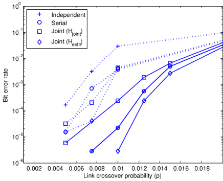
Figure 5: Different length-500, rate-1/2, LDPC codes are used to encode $\mathbf{u}_{A}$ and $\mathbf{u}_{B}$ which are transmitted over the network in Fig. 4. Shown is the bit error rate performance of packet $A$ (solid curves) and packet $B$ (dotted curves) using the four different decoding schemes. The link crossover probabilities are $p$ with the exception of link $2\rightarrow 6$ which has crossover probability $3p$.

Fig. 5 shows the error correction performance of the various decoding methods when $\mathbf{u}_{A}$ and $\mathbf{u}_{B}$ are encoded with different randomly chosen LDPC codes. We can see that independently decoding with the network and then channel codes performs as expected, returning poor performances for the decoding of $\mathbf{u}_{B}$, since it is corrupted by both the errors on $\widetilde{\mathbf{c}_{A}}$ and those on $\widetilde{\mathbf{c}_{AB}}$. Also as expected, using serial decoding or either version of joint decoding, $\widetilde{\mathbf{c}_{B}}$ is only corrupted by the errors from $\widehat{\mathbf{c}_{A}}$ that remained after decoding and so the decoding performance of $\mathbf{u}_{B}$ is significantly improved.

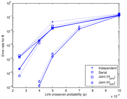
Figure 6: Different length-500, rate-1/2, LDPC codes are used to encode $\mathbf{u}_{A}$ and $\mathbf{u}_{B}$ which are transmitted over the network in Fig. 4. Shown is the bit error rate performance of packet $A$ (solid curves) and packet $B$ (dotted curves) using the four different decoding schemes. The link crossover probabilities are $p$ with the exception of link $2\rightarrow 6$ which now has crossover probability $12p$.

Fig. 6 emphasizes the benefit that joint decoding, by using the network code as part of a larger error correction code, can provide to $\mathbf{u}_{A}$ over decoding with the channel code alone. In this simulation the network is modified to increase the crossover probability on link $2\rightarrow 6$ to be $12p$.

Overall, serial decoding performs equally as well as independent network-then-channel decoding for $A$ but improves the performance of $B$. The error rate of the first joint decoding scheme however, is poorer than that of serial decoding for $A$ as it is hampered by the 4-cycles in the parity-check matrix $H_{AB}$. The extended joint decoding scheme, which is able to jointly decode $A$ and $B$ using a cycle free Tanner graph, outperforms all the other schemes for both $A$ and $B$.

The network coding performed at node 4 to improve the throughput of the network has the unavoidable effect of reducing the BER performance of packet $B$ (when compared to a network which uses two channel transmissions at node 4 to send $A$ and $B$ separately to node 5). However, by using joint decoding, this loss in performance can be significantly reduced and, furthermore, the network coding can even be used to improve the BER performance of packet $A$ (compared to the network without network coding).

Although joint decoding can not improve the rate region (in the Shannon sense, i.e., rates with error probability approaching zero using infinitely long code length) for $B$ over that of serial decoding, simulation results show a bit error rate performance improvement for $B$ when joint decoding with $H_{\text{extn}}$ is used, showing that by jointly decoding $A$ and $B$ the convergence performance of $B$ can be improved. Or put another way, if $\mathbf{c}_{A}$ is received without error there will be no improvement in the performance of joint over serial decoding of $\mathbf{c}_{B}$. However, using a finite code length, where errors occur in $\mathbf{c}_{A}$, joint decoding can remove more errors from $\mathbf{c}_{A}$ so fewer errors remain to corrupt $\mathbf{c}_{B}$. Furthermore, the decoding of $A$ and $B$ can be successively improved iteratively using a better estimate of $A$ to improve the decoding of $B$ and vice versa.

V-B Complexity

The decoding schemes proposed here do not employ channel codes in the intermediary network nodes, so the network complexity remains the same for all decoding schemes. Sources $A$ and $B$ are encoded independently by the encoder in the same way for each scheme and so the source node complexity also does not change. The only increase in complexity for the joint decoding schemes occurs for the decoder at the destination node.

In general, the complexity of the sum-product decoding algorithm is a linear function of the number of non-zero entries in the parity-check matrix. For $(3,6)$-regular length $n$ LDPC codes the total number of non-zero parity-check matrix entries in $H_{A}$ and $H_{B}$ is $3n$ each. Thus, the independent and serial decoding schemes have a total of $6n$ non-zero parity-check matrix entries (over both matrices), while the joint network / channel decoding matrix can have up to $6n$ additional non-zero entries (if there are no entries overlapped in $H_{A}$ and $H_{B}$), and the extended joint decoding matrix has $3n$ additional non-zero entries. Thus, using rate half codes the number of non-zero parity-check matrix entries is $6n$ for independent decoding, between $6n$ (common channel codes) and $12n$ (completely disjoint parity-check matrices) for joint decoding and $9n$ for extended joint decoding. For all the schemes, decoding complexity remains linear in the block length, and while the joint decoding schemes have a slightly higher decoding complexity per iteration, their improved performance means that fewer decoder iterations are actually required.

VI Conclusion

In this paper we have considered decoding schemes for low complexity networks, where a message is encoded at the source node and decoded at the destination node, and intermediate nodes perform network coding operations, in our case modulo-2 addition, but no channel coding. We have investigated three potential decoding schemes for the destination: (1) independent decoding where the destination decodes data from each link independently, (2) serial decoding where the destination decodes data from each link independently, but in series and by using the knowledge of previously decoded links, and (3) joint decoding where the destination jointly decodes all data from all the links simultaneously.

In networks with noisy links and low-complexity intermediary nodes it can still be of benefit to perform a simple network coding strategy, involving the XOR of (noise-corrupted) codewords rather than messages, and use joint decoding at the destination to retrieve the transmitted codewords. We saw that our proposed decoding scheme improves the error correction performance of the network over the independent and the serial decoding schemes, and does so without adding network complexity. This is achieved by describing a joint network code / channel code at the destination node and decoding with iterative sum-product decoding. The new schemes require no channel coding at the intermediary network nodes and only a small amount of additional decoding complexity at the destination node. The joint decoding produces improved error correction performances and can significantly improve decoder speed.

References

- [1] Ahlswede R, Cai N, Li SY, Yeung RW. Network information flow. IEEE Transactions on Information Theory July 2000; 46(4):1204–1216.
- [2] Song L, Yeung RW, Cai N. A separation theorem for single-source network coding. IEEE Transactions on Information Theory May 2006; 52(5):1861–1871.
- [3] Borade S. Network information flow: Limits and achievability. Proceedings of IEEE International Symposium on Information Theory, Lausanne, Switzerland, 2002; 661–666.
- [4] Effros M, Medard M, Ho T, Ray S, Karger D, Koetter R, Hassibi B. Linear network codes: A unified framework for source, channel, and network coding. DIMACS Series in Discrete Mathematics and Theoretical Computer Science, vol. 66, Rutgers University, Piscataway, NJ, USA, 2003; 197–216.
- [5] Hausl C. Joint network-channel coding for the multiple-access relay channel based on turbo codes. European Transactions on Telecommunications 2009; 20:175–181.
- [6] Hausl C, Hagenauer J. Iterative network and channel decoding for the two-way relay channel. Proceedings of the 2006 IEEE International Conference on Communications, vol. 4, 2006; 1568–1573.
- [7] Hausl C, Schreckenbach F, Oikonomidis I, Bauch G. Iterative network and channel decoding on a Tanner graph. Proceedings of the 43rd Annual Allertion Conference on Communication, Control, and Computing, Monticello, Illinois, USA, 2005.
- [8] Chakrabarti A, de Baynast A, Sabharwal A, Aazhang B. Low density parity check codes for the relay channel. IEEE Journal on Selected Areas in Communications February 2007; 25(2).
- [9] Hu J, Duman TM. Low density parity check codes over wireless relay channels. IEEE Transactions on Wireless Communications September 2007; 6(9):3384–3394.
- [10] Razaghi P, Yu W. Bilayer low-density parity-check codes for decode-and-forward in relay channels. IEEE Transactions on Information Theory October 2007; 53(10):3723–3739.
- [11] Bao X, Li J. A unified channel-network coding treatment for user cooperation in wireless ad-hoc networks. Proceedings of the IEEE International Symposium on Information Theory, Seattle, Washington, USA, 2006; 202–206.
- [12] Tran T, Nguyen T, Bose B. A joint network-channel coding technique for single-hop wireless networks. Proceedings of the Fourth Workshop on Network Coding, Theory and Applications (NETCOD), 2008; 1–6.
- [13] Langberg M, Sprintson A, Bruck J. Network coding: a computational perspective. IEEE Transactions on Information Theory January 2009; 55(1):147–157.
- [14] Sankaranarayanan L, Kramer G, Mandayam NB. Hierarchical sensor networks: Capacity bounds and cooperative strategies using the multiple-access relay channel model. Proceedings of the First Annual IEEE Communications Society Conference on Sensor and Ad Hoc Communications and Networks (IEEE SECON), 2004; 191–199.
- [15] Yang S, Koetter R. Network coding over a noisy relay: a belief propogation approach. Proceedings of the IEEE International Symposium on Information Theory, Nice, France, 2007; 801–804.
- [16] Yang Z, Tong L. On the error exponent and the use of LDPC codes for cooperative sensor networks with misinformed nodes. Information Theory, IEEE Transactions on Sept 2007; 53(9):3265–3274, doi:10.1109/TIT.2007.903116.
- [17] Elias P. Coding for noisy channels. IRE Conv. Rec. Mar 1955; 4:37–46.
- [18] Liao H. Multiple access channel. PhD Thesis, Univ. Hawaii Honolulu, HI 1972.
- [19] Ahlswede R. The capacity of a channel with two senders and two receivers. Ann. Probab. Oct 1974; 2:805–814.
- [20] Ong L, Johnson SJ, Kellett CM. Achievable rate regions of the butterfly network with noisy links and end-to-end error correction. Proc. IEEE Inf. Theory Workshop (ITW), Taormina, Italy, 2009; 554–558.
- [21] Gallager RG. Low-Density Parity-Check Codes. MIT Press: Cambridge, MA, 1963.
- [22] MacKay DJC. Good error-correcting codes based on very sparse matrices. IEEE Trans. Inform. Theory March 1999; 45(2):399–431.
- [23] Chung SY, Forney GD Jr, Richardson TJ, Urbanke RL. On the design of low-density parity-check codes within dB of the Shannon limit. IEEE Commun. Letters February 2001; 5(2):58–60.
- [24] MacKay DJC, Neal RM. Near Shannon limit performance of low density parity check codes. Electron. Lett. March 1996; 32(18):1645–1646. Reprinted Electron. Lett, vol. 33(6), pp. 457–458, March 1997.
- [25] Tanner RM. A recursive approach to low complexity codes. IEEE Trans. Inform. Theory September 1981; IT-27(5):533–547.
- [26] Johnson SJ, Kellett CM. Joint network and channel coding for cooperative networks. Proceedings of the Australasian Telecommunication Networks and Applications Conference, Christchurch, New Zealand, 2007.
- [27] Kang J, Zhou B, Ding Z, Lin S. LDPC coding schemes for error control in a multicast network. Proceedings of the IEEE International Symposium on Information Theory, Toronto, Canada, 2008; 822–826.
- [28] Neal RM. www.cs.toronto.edu/radford/.