Effectiveness and detection of
denial of service attacks in Tor

Abstract.

Tor is one of the more popular systems for anonymizing near real-time communications on the Internet. Borisov et al. proposed a denial of service based attack on Tor (and related systems) that significantly increases the probability of compromising the anonymity provided. In this paper, we analyze the effectiveness of the attack using both an analytic model and simulation. We also describe two algorithms for detecting such attacks, one deterministic and proved correct, the other probabilistic and verified in simulation.

Copyright ACM, 2013. This is the author’s version of the work. It is posted here by permission of ACM for your personal use. Not for redistribution. The definitive version was published in Transactions on Information and System Security, Volume 11 (2013), http://dx.doi.org/10.1145/2382448.2382449.

1. Introduction

A low-latency anonymous communication system attempts to allow near-real-time communication between hosts while hiding the identity of these hosts from various types of observers (including each other). Such a system is useful whenever communication privacy is desirable — personal, medical, legal, governmental, or financial applications all may require some degree of privacy. Dingledine, Mathewson, and Syverson (2004a) developed the Onion Routing network Tor for such communication. Tor anonymizes communication by sending it along paths of anonymizing proxies, encrypting messages in layers so that each proxy only knows its neighbors in the path.

Syverson et al. (2000) showed that such systems are vulnerable to a passive adversary (one who does not modify traffic in any way) who controls the first and last proxies along such a path; roughly speaking, the attack involves a cross-correlation of timing data. Active attacks, and in particular, denial of service (DoS) attacks, can increase the power of an otherwise limited attacker. For example, Dingledine, Shmatikov, and Syverson (2004b) analyzed the impact of DoS on different configurations of mix networks. The Crowds design paper Reiter and Rubin (1998) examined the impact of circuit interruptions on anonymity. And the original Tor design paper describes various denial of service attacks. More recently, Borisov et al. (2007) showed that an adversary willing to engage in denial of service (DoS) could increase her probability of compromising anonymity. When a path is reconstructed after a denial of service, new proxies are chosen, and thus the adversary has another chance to be on the endpoints of the path.

In this paper we analyze the denial-of-service attack in detail and propose two detection algorithms. In Section 2 we give a careful description of the attack in terms of a number of parameters that the attacker might vary to avoid detection (our model includes Borisov et al.’s attacker and the passive attacker as special cases). In Section 3 we assess the effectiveness of the attacker as a function of these parameters. We compare our analytic results to a simulation of the attacker based on replaying data collected from the deployed Tor network. In Section 4 we prove that an adversary engaging in the DoS attack in an idealized Tor-like system can be detected by probing at most $3n$ paths in the system, where $n$ is the number of proxies in the system. We give a more practical algorithm in Section 5, implement it in simulation, and show that it detects DoS attackers with low error rate. In Section 6 we discuss attackers that do not fit our model perfectly and show how our detection algorithms might cope with such attackers. In Section 7 we discuss issues related to deploying the detection algorithms we describe. Finally, attacking and defending anonymity networks is an arms race; in Section 8 we discuss other attempts to detect and defend against various kinds of attacks. In particular, we compare our more practical detection algorithm to the “client-level” algorithm for avoiding compromised tunnels described by Das and Borisov (2011) in that section.

2. The Denial of Service Attack

We model the Tor network with a fully connected undirected graph. The vertices of the graph represent the Tor nodes (or relays), and the edges represent network connections between nodes. We define $n$ to be the number of vertices. For a DoS attack, we assume that the attacker controls some subset of the relays; we may also use the term compromised to describe such relays.

A Tor client creates circuits (also referred to as paths or tunnels) consisting of three nodes; in our model, this equates to a path containing three vertices (in order) and the corresponding edges between them. The first node is referred to as the entry node and the last as the exit node. Application level communications between an initiator and a responder are then passed through the circuit. We assume that if the adversary controls the entry and exit nodes on a circuit, then she can in fact determine whether or not the traffic passing through the entry node is the same as the traffic passing through the exit node (and hence she can match the initiator with the recipient of the traffic). An early version of such an attack is given by Levine et al. (2004) and a more sophisticated version by Murdoch and Zieliński (2007). A circuit is compromised if at least one node on the circuit is compromised and the circuit is controlled if both the entry and exit nodes are compromised.

Syverson et al. (2000) observe that if all nodes may act as exit nodes, then a passive adversary controls a circuit with probability $\frac{c^{2}}{n^{2}}$, where $c$ is the number of nodes controlled by the attacker. Since controlling middle nodes is of little use, we might also consider an attacker who selectively compromises exit nodes. In this case the probability of control is $\frac{c^{2}}{nc^{\prime}}$, where $c^{\prime}$ is the number of compromised exit nodes. Levine et al. (2004) observe that if long-lived connections between an initiator and responder are reset at a reasonable rate then such an attack will be able to compromise anonymity with high probability within $O(\frac{n^{2}}{c^{2}}\ln n)$ resets.

But Tor’s node-selection algorithm is more sophisticated than portrayed in these models. Nodes are assigned flags by directory servers, and among these flags are “Guard” and “Exit.” Entry and exit nodes will only be chosen from nodes that are flagged Guard and Exit, respectively, and a given guard, middle, or exit node is chosen with probability proportional to its contribution to the total guard, network, or exit bandwidth. Furthermore, unless the total bandwidth contributed by exit nodes is greater than $1/3$ of the total network bandwidth, exit nodes will not be chosen for any other position on a circuit. If the contribution is $t>1/3$, then the probability with which an exit node will be chosen for a non-exit position is weighted by $t-1/3$, so $t$ must be significantly greater than $1/3$ for an exit node to be chosen in a non-exit position with any non-trivial probability. The same applies to guard nodes.

Even further, guard nodes are not chosen each time a circuit is built by a client. Instead, a client constructs a list of guard nodes (currently of length $3$) chosen by the above algorithm when first started, and thereafter always choses entry nodes uniformly at random from that list when constructing circuits (guard nodes were first described by Wright et al. (2003)). New nodes are added to the list only if there are fewer than three reachable nodes in the list, and a node is removed from the list only if it has not been reachable for some time. This protocol is intended to reduce the likelihood that a client eventually constructs a circuit that is controlled by an attacker. If new entry nodes were chosen for every circuit, then the probability that a compromised entry node is chosen converges to $1.0$. The guard node list changes the calculus a bit: the probability of choosing a compromised node to put into the list is (hopefully) low, and if there are no such nodes in the list, then the client will never be subject to a traffic confirmation attack of the sort referenced earlier. However, if there is a compromised node in the list, then any circuit created by the client will have a compromised entry node with fairly high probability.

In order to further improve the chances of controlling a circuit, a number of researchers Overlier and Syverson (2006); Bauer et al. (2007); Borisov et al. (2007) have suggested that compromised nodes that occur on paths in which they are not the first or last node artificially create a reset event by dropping the connection. Borisov et al. (2007) analyze the following version of this attack on Tor. If the attacker controls one of the relays of a given circuit, she can use various timing techniques to determine if she controls both endpoints. If she does not, she kills the circuit, forcing the client to build another. In the terminology we introduce below, Borisov et al.’s attacker can be described as killing circuits that are compromised but not controlled in an effort to increase the number of circuits that she controls.

Killing a large number of circuits may make an attacker’s nodes stand out from other nodes on the network, so the attacker may try to “fit in” by not always killing compromised but uncontrolled circuits. In the notation introduced below, the attacker may have $p_{\mathrm{kill}}<1.0$. At the same time, nodes on the Tor network do fail, for example because they have reached bandwidth limits or because of network failures. So an attacker might also occasionally kill circuits that she controls in an attempt to look “more realistic.” In the notation below, the attacker may have $p_{\mathrm{permit}}<1.0$.

So some relevant parameters for a denial-of-service attacker are the bandwidth contributed by attacker nodes (as this determines the probability with which her nodes are chosen as part of a circuit) and the probabilities of killing compromised uncontrolled circuits and permitting controlled circuits. More specifically, we identify the following partial list of parameters necessary to model the attacker:

1. $g$, the ratio of compromised guard bandwidth to total guard bandwidth.

2. $e$, the ratio of compromised exit bandwidth to total exit bandwidth.

3. $p_{\mathrm{kill}}$, the probability that the attacker kills a compromised but uncontrolled circuit.

4. $p_{\mathrm{permit}}$, the probability that the attacker permits a circuit that she controls to be used.

We make the following assumptions about the attacker:

1. $g>0$, $e>0$, and $p_{\mathrm{permit}}>0$ (otherwise the attacker can never control a circuit, or always kills any circuit she controls).

2. The attacker only controls nodes with the Guard or Exit flags (or both) set.

3. The attacker is local—i.e., the attacker can observe and modify traffic passing through nodes she controls, but not other traffic.

So the attacker described by Borisov et al. has $(p_{\mathrm{kill}},p_{\mathrm{permit}})=(1.0,1.0)$ and the passive attacker who never kills any circuits has $(p_{\mathrm{kill}},p_{\mathrm{permit}})=(0.0,1.0)$.

Parameters describing the attacker
$g$/$e$/$z$	The ratio of compromised guard/exit/guard-exit bandwidth to total guard bandwidth.
$p_{\mathrm{kill}}$	The probability that the attacker kills a compromised but uncontrolled circuit.
$p_{\mathrm{permit}}$	The probability that the attacker permits (does not kill) a controlled circuit.
Parameters describing the network
$n$	The number of relays in the Tor network.
$\gamma$/$\eta$/$\zeta$	The ratio of guard/exit/guard-exit bandwidth to total bandwidth.
Other quantities and terms
$K$	The number of circuit-creation attempts a client makes before giving up.
Compromised circuit	The attacker controls at least one relay on the circuit.
Controlled circuit	The attacker controls the entry and exit relays of the circuit.

Table 1. Notation and terminology used in Section 2.

We also make the following assumptions about the Tor network:

1. The only reason for relay failure is a compromised relay killing a circuit.

2. Paths are chosen with replacement.

Of course, the first assumption is unreasonable, and the second is false: not only are paths chosen without replacement, but in fact no two nodes on a path can belong to the same /16 subnetwork. We make these assumptions about the network because modeling the actual behavior in our analytic model of the attacker is extremely difficult. We assess the impact of these two assumptions on our analytic model in Section 3.2.

Tor’s modified bandwidth-weighting algorithm chooses each relay with probability proportional to its weighted bandwidth, where the weight assigned to a relay depends on the position being selected for (guard, middle, or exit) and the flags of the relay. To fully describe the attacker, we need to compute these probabilities. A guard-only relay is one with the Guard flag set and the Exit flag not set; this is in distinction to a guard relay, which is one in which the Guard flag is set, irrespective of the Exit flag. We define exit-only and exit relays similarly. A guard-exit relay is one with both flags set. The bandwidth weights are defined in terms of the following values:

• $G$, $E$, and $T$, the guard-, exit-, and total bandwidth of the network, respectively;

• $\gamma=G/T$; $\eta=E/T$.

• $w_{G_{0}}=1-1/3\gamma$; $w_{E_{0}}=1-1/3\eta$; and $w_{Z}=w_{G_{0}}w_{E_{0}}=(1-1/3\gamma)(1-1/3\eta)$.

The various weights are given in Table 2.

		Flags
		Guard-only	Exit-only	Guard-exit	None
	Guard	1.0	0.0	$w_{E_{0}}$	0.0
Position	Middle	$w_{G_{0}}$	$w_{E_{0}}$	$w_{Z}$	1.0
	Exit	0.0	1.0	$w_{G_{0}}$	0.0

Table 2. Bandwidth weights assigned by Tor based on position and flags.

A node $R$ is chosen for a given position with probability $b^{\prime}/T^{\prime}$, where $b^{\prime}$ is the weighted bandwidth of $R$ and $T^{\prime}$ is the total bandwidth of all nodes weighted for that position. So to compute the probability that a compromised node is chosen in any position, we have to consider the possible combination of flags of that node. To that end, define

• $G_{0}$, $E_{0}$, and $Z$ to be the guard-only, exit-only, and guard-exit bandwidth, respectively;

• $\gamma_{0}=G_{0}/T$; $\eta_{0}=E_{0}/T$; $\zeta=Z/T$.

• $G_{0}^{\prime}$, $E_{0}^{\prime}$, and $Z^{\prime}$ to be the compromised guard-only, exit-only, and guard-exit bandwidth, respectively;

• $\gamma_{0}^{\prime}=G_{0}^{\prime}/T$; $\eta_{0}^{\prime}=E_{0}^{\prime}/T$; $\zeta^{\prime}=Z^{\prime}/T$.

• $z=Z^{\prime}/Z$; this give a parameter for compromised guard-exit bandwidth corresponding to $g$ and $e$.

Some of these parameters are defined in terms of the others:

• $\gamma_{0}=\gamma-\zeta$ and $\eta_{0}=\eta-\zeta$.

• $\zeta^{\prime}=z\zeta$.

• $\gamma_{0}^{\prime}=g\gamma-z\zeta$ and $\eta_{0}^{\prime}=e\eta-z\zeta$. We can see this by noting that $\gamma_{0}^{\prime}T=G_{0}^{\prime}=gG-zZ$, from which the expression for $\gamma_{0}^{\prime}$ follows. The expression for $\eta_{0}^{\prime}$ is derived similarly.

Thus the bandwidth contributed by guards and exits is $G+E-Z=G_{0}+E_{0}+Z$. We use these parameters to describe the probability of choosing compromised relays as follows:

• A compromised guard node is chosen with probability

  $$g^{*}=\frac{G_{0}^{\prime}+Z^{\prime}w_{E_{0}}}{G_{0}+Zw_{E_{0}}}=\frac{\gamma_{0}^{\prime}+\zeta^{\prime}w_{E_{0}}}{\gamma_{0}+\zeta w_{E_{0}}}=\frac{g\gamma-z\zeta(1-w_{E_{0}})}{\gamma-\zeta(1-w_{E_{0}})}.$$

  The first equality follows by dividing numerator and denominator by $T$.

• A compromised middle node is chosen with probability

  $$m =\frac{G_{0}^{\prime}w_{G_{0}}+E_{0}^{\prime}w_{E_{0}}+Z^{\prime}w_{Z}}{G_{0}w_{G_{0}}+E_{0}w_{E_{0}}+Zw_{Z}+(T-G_{0}+E_{0}+Z)}$$

  $$=\frac{G_{0}^{\prime}w_{G_{0}}+E_{0}^{\prime}w_{E_{0}}+Z^{\prime}w_{Z}}{T-(G_{0}(1-w_{G_{0}})+E_{0}(1-w_{E_{0}})+Z(1-w_{Z})}$$

  $$=\frac{\gamma_{0}^{\prime}w_{G_{0}}+\eta_{0}^{\prime}w_{E_{0}}+\zeta^{\prime}w_{Z}}{1-(\gamma_{0}(1-w_{G_{0}})+\eta_{0}(1-w_{E_{0}})+\zeta(1-w_{Z}))}$$

  $$=\frac{(g\gamma-z\zeta)w_{G_{0}}+(e\eta-z\zeta)w_{E_{0}}+z\zeta w_{Z}}{1-\bigl{(}(\gamma-\zeta)(1-w_{G_{0}})+(\eta-\zeta)(1-w_{E_{0}})+\zeta(1-w_{Z})\bigr{)}}$$

• A compromised exit node is chosen with probability

  $$e^{*}=\frac{E_{0}^{\prime}+Z^{\prime}w_{G_{0}}}{E_{0}+Zw_{G_{0}}}=\frac{\eta_{0}^{\prime}+\zeta^{\prime}w_{G_{0}}}{\eta_{0}+\zeta w_{G_{0}}}=\frac{e\eta-z\zeta(1-w_{G_{0}})}{\eta-\zeta(1-w_{G_{0}})}.$$

Taking into account the fact that the bandwidth weighting factors are defined in terms of the other parameters, a full specification of the attacker for the purposes of our model consists of:

1. $g$, $e$, and $z$, the guard-, exit-, and guard-exit bandwidth contributed by compromised nodes;

2. $\gamma$, $\eta$, and $\zeta$, the ratios of guard-, exit-, and guard-exit bandwidth to total bandwidth of the network;

3. $p_{\mathrm{kill}}$ and $p_{\mathrm{permit}}$, the kill- and permit- probabilities of the attacker.

This completes our description of the attacker.

3. Effectiveness of the attack

3.1. Theoretical results

We give a theoretical assessment of the effectiveness of the denial-of-service attack in this section. To do so, we fix the parameters describing the attacker and consider the following experiment conducted by an imaginary client:

1. The client repeatedly chooses a path according to the path-selection algorithm described earlier until he choses a successful path.

   • The path is unsuccessful if it is killed by the attacker (such a circuit must be compromised or controlled).

   • The path is successful otherwise.

2. If the client chooses $K$ unsuccessful paths for some fixed $K$, then he gives up.

We say that the attacker eventually controls the client’s path if the client chooses a successful path that is controlled by the attacker. We can then ask what the probability is that the attacker eventually controls the client’s path.

We wish to focus on the parameters $g$, $e$, $p_{\mathrm{permit}}$, and $p_{\mathrm{kill}}$. To do so, we fix $\gamma=.70$, $\eta=.40$, and $\zeta=.30$, values that we measured on the deployed Tor network in mid June 2011 (so we assume that the attacker’s nodes do not have a significant impact on the total guard or exit bandwidth fraction).

The values of $g$, $e$, and $z$ are not independent, because compromised guard-exit bandwidth (as described by $z$) imposes a lower bound on compromised guard bandwidth and exit bandwidth. To achieve some desired values of $g$ and $e$, the attacker can compromise relays with a strategy that ranges the spectrum from compromising no guard-exit relays to compromising as many as possible. Although the flags are assigned by Tor’s directory authorities, it does not seem difficult to configure a relay and behave in such a way that either or both flags will be assigned. For now, we focus on the “prefer guard-exit” strategy, returning to the “avoid guard-exit” strategy later. To achieve target compromise ratios $g$ and $e$, the attacker compromises guard-exit relays until the compromised guard or exit bandwidth ratio is either $g$ or $e$, respectively. She then compromises/runs relays of the other type until that desired bandwidth ratio is achieved. In this case, $z$ is an “observed” value, which our analytic model does not handle directly. Based on simulations of this strategy (see Section 3.2), we have observed that this approach typically results in $z\approx 1.5g$ when $g=e$ and $g\geq.05$ (the ratio is larger for smaller values of $g$, reaching about $2.5$ for $g=.01$). So for our analytic evaluation, we will take $z=1.5g$.

The appropriate value of $K$ depends on the typical length of time it takes for a circuit-creation attempt to fail and the time it would normally take a client application to time out waiting for a connection and hence give up. In our measurements, a failed circuit-creation attempt either takes very little time (around $.5$ seconds) or a very long time (around $60$ seconds). Thus if there are attacks currently running, we can model the attacker by taking $K$ between $2$ and $120$. Since killing uncontrolled circuits quickly gives the attacker more chances to control the client’s circuit, we choose $K=120$. Of course, this represents a very efficient attacker; we return to this choice at the end of Section 3.2.

We now determine the probability that the attacker eventually controls the client’s path. If there are $0$ attackers in the client’s guard-node list, then the probability of eventual control is $0$. Since the attacker eventually controls the client’s circuit if there is some $i<K$ such that the client chooses $i$ unsuccessful paths followed by a path that is controlled by the attacker, the probability of eventual control with $j\geq 1$ attackers in the guard-node list is

$$\Pr[\text{even.\ ctrl., $j$ attackers}]=\sum_{i=0}^{K-1}u_{j}^{i}\left(p_{\mathrm{permit}}\cdot\frac{j}{3}\cdot e^{*}\right)=\left(p_{\mathrm{permit}}\cdot\frac{j}{3}\cdot e^{*}\right)\left(\frac{u_{j}^{K}-1}{u_{j}-1}\right)$$

where $u_{j}=u_{j}(C)$ is the probability that the path $C$ is unsuccessful when the client has $j$ attacker nodes in his guard node list. We compute $u_{j}(C)$ as follows:

$$u_{j}(C) =(1-p_{\mathrm{permit}})\cdot\Pr[\text{$C$ controlled}]+p_{\mathrm{kill}}\cdot\Pr[\text{$C$ compr., uncontr.}]$$

$$=(1-p_{\mathrm{permit}})\left(\frac{j}{3}e^{*}\right)+p_{\mathrm{kill}}\cdot\left(\frac{j}{3}\Bigl{(}1-e^{*}\Bigr{)}+\Bigl{(}1-\frac{j}{3}\Bigr{)}e^{*}+\Bigl{(}1-\frac{j}{3}\Bigr{)}(1-e^{*})m\right).$$

This is derived as follows. $C$ is controlled if the client chooses a compromised guard node (probability $j/3$) and a compromised exit node (probability $e^{*}$). $C$ is compromised and uncontrolled if either the client chooses a compromised guard node and an uncompromised exit node (probability $(j/3)(1-e^{*})$), an uncompromised guard node and a compromised exit node (probability $(1-j/3)(e^{*})$), or uncompromised guard and exit nodes and a compromised middle node (probability $(1-j/3)(1-e^{*})m$).

Taking into account the probability of having $j$ attackers in the client’s guard-node list,

$$\Pr[\text{even.\ ctrl.}]=\sum_{j=1}^{3}{3\choose j}(1-g^{*})^{3-j}(g^{*})^{j}\left(p_{\mathrm{permit}}\cdot\frac{j}{3}\cdot e^{*}\right)\left(\frac{u_{j}^{K}-1}{u_{j}-1}\right).$$

Figure 1 shows the contour plot of the eventual control probability for the naive denial-of-service attacker ($(p_{\mathrm{permit}},p_{\mathrm{kill}})=(1.0,1.0)$) and the passive attacker ($(p_{\mathrm{permit}},p_{\mathrm{kill}})=(1.0,0.0)$) in terms of $g$ and $e$, with the other parameters fixed as described above. As expected, the naive attacker controls significantly more circuits than the passive attacker, consistently about $2.5$ times as many, regardless of $g$ and $e$. Perhaps something that is not so obvious without this analysis is that for high compromise ratios, the attacker gets more bang for her buck by compromising additional exit bandwidth rather than guard bandwidth.

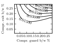
(a) Naive attacker

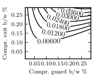
(b) Passive attacker

Figure 1. Eventual control probability for the naive ($(p_{\mathrm{permit}},p_{\mathrm{kill}})=(1.0,1.0)$) and passive ($(p_{\mathrm{permit}},p_{\mathrm{kill}})=(1.0,0.0)$) attackers in terms of guard and exit node bandwidth contributed by the attacker.

We can also vary $p_{\mathrm{kill}}$ and $p_{\mathrm{permit}}$ while keeping $g$ and $e$ constant. Figure 2 shows the contour plot of the eventual control probability for a low-resource attacker ($g=e=.01$) and a high-resource attacker $(g=e=.10$).

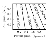
(a) Low-resource attacker

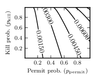
(b) High-resource attacker

Figure 2. Eventual control probability for low resource ($g=e=.01$) and high-resource ($g=e=.1$) attackers.

We see that the low-resource attacker with $(p_{\mathrm{permit}},p_{\mathrm{kill}})=(1.0,1.0)$ eventually controls about $.007\%$ of circuits, whereas the comparable high-resource attacker eventually controls about $.9\%$ of circuits. Increasing compromised guard and exit bandwidth by a factor of $10$ increases the number of eventually-controlled circuits by a factor of more than $100$.

So what are the resources required by our high-resource attacker? At the time of our measurements, the guard-only, exit-only, and guard-exit bandwidths of the deployed network were about $1100$ MB/s, $251$ MB/s, and $751$ MB/s, respectively, so our attacker would have to provide about $185$ MB/s with guards and $100$ MB/s with exits. An attacker following our strategy of preferring guard-exit relays would therefore have to provide about $100$ MB/s of guard-exit bandwidth and $85$ MB/s of guard-only bandwidth. If she tries to keep a low profile by running her nodes at the median bandwidth for each type (about $435$ KB/s and $455$ KB/s for guard-exit and guard-only, respectively), she would have to run about $235$ guard-exits and $191$ guard-only relays. If instead she runs nodes in the $90$-th percentile by bandwidth (about $10$ MB/s and $9.5$ MB/s for guard-exit and guard-only, respectively), she would need to run about $10$ guard-exits and $8$ guard-only relays, which certainly seems well within reason. Our low-resource attacker really is low-resource, provided she has sufficient bandwidth to run nodes in the $90$-th percentile: she need only run one guard-exit and one guard-only relay.

However, these very low numbers of relays are misleading, because in practice no relay can appear twice in a single circuit. If the attacker has very few nodes, then choosing paths without replacement could have an adverse effect on the attacker. For example, if the chosen guard makes up a significant contribution to the attacker’s guard-exit bandwidth, then the probability of choosing a compromised exit may be much lower than that predicted by this model. This is a general problem for the attacker who has any guard-exit relays; if one of them is chosen as a guard relay, then that decreases the attacker’s available exit bandwidth, thereby reducing the probability that the client’s circuit is eventually controlled. The reduction in effectiveness is significant in this analytic model. We have performed the same analyses with an attacker who compromises no guard-exit relays, and she is predicted to be $5$–$8$ times more effective, depending on the specific choices of the various parameters. However, this is almost certainly an over-estimate, because our analytic model assumes that there is enough bandwidth to meet the attacker’s goals. This is not the case; for example, in the data we use for our replay simulation in the next section, exit-only relays with bandwidth in the $90$-th percentile and below yield just $3.5\%$ of total exit bandwidth, so our attacker would not be able to have $e>.035$ with this strategy.

3.2. Simulation results

As we have already mentioned, our model makes a number of unrealistic assumptions. It does not take into account the fact that relays fail for reasons unrelated to an attacker; for example, there may be transient network failures, a relay may have reached its bandwidth cap, etc. It assumes that paths are chosen with replacement, whereas Tor circuits are chosen without replacement. And it assumes that there is sufficient bandwidth for the attacker to compromise her desired ratios with any combination of guard-only, exit-only, and guard-exit relays. To assess the quality of our analytic model in light of these assumptions, we implement a replay simulation as described below and compare the proportion of eventually-controlled circuits predicted by the analytic model to the proportion that are eventually controlled in the simulation.

Define a lifecycle for a relay $R$ to be a function $\ell_{R}:\{0,1,\dotsc\}\to\{-1,0,1\}$. The idea is that we “probe” $R$ some number of times, and $\ell_{R}(t)$ is the result of the $t$-th probe. A probe consists of constructing a circuit of the form $(G,R,E)$ and downloading a small file through the circuit, where $G$ and $E$ are relays that we control. Probe $t$ succeeds ($\ell_{R}(t)=1$) if the file is successfully downloaded and otherwise the probe fails. A probe may fail because $R$ is not in the consensus at time $t$ ($\ell_{R}(t)=-1$) or for some other reason such as a transient network failure, bandwidth limiting, etc. ($\ell_{R}(t)=0$). A trial consists of probing each relay in the network—i.e., $\{\ell_{R}(t)\mid\text{$R$ a relay}\}$ for some fixed $t$. We collect lifecycle data on each relay in the deployed network by conducting some number of trials; for the results reported here, we conducted $100$ trials over a period of about $48$ hours.

With this lifecycle data in hand, we can simulate the denial-of-service attack as follows:

1. Mark some number of the relays that are in the consensus in the first trial as attackers; these relays are chosen according to requested values of the parameters $g_{0}$, $e_{0}$, and $z$ as described in our model of the attacker. Because relays have discrete bandwidths, the actual ratio of compromised bandwidth will differ somewhat from these requested values. We compromise relays starting at the top $90$-th percentile of bandwidth without regard to actual reliability.

2. Attempt to build a circuit as follows:

   1. Select $3$ guard relays from those relays $R$ that have the Guard flag set in trial $0$.

   2. Choose a trial $t$ at random and try to build a circuit up to some maximum number of times (corresponding to the parameter $K$ in our analytic model).

      1. Select an entry relay uniformly at random from the $3$ guard relays.

      2. Select middle node and exit relays from those relays $R$ such that $\ell_{R}(t)\not=-1$ (exit relays must have the Exit flag set). Choose these two relays so that all three relays are distinct.

      3. If any of the relays $R$ has $\ell_{R}(t)=0$, the build attempt fails; try again.

      4. If the circuit is compromised but not controlled, the attacker kills it with probability $p_{\mathrm{kill}}$; if it is killed, try again.

      5. If the circuit is controlled, the attacker kills it with probability $1-p_{\mathrm{permit}}$; if it is killed, try again.

      6. Otherwise, the build attempt is successful.

We can then analyze how many of the circuit construction attempts result in circuits that are eventually controlled by the attacker.

We show one such comparison in Figure 3. For this analysis we consider compromise ratios $r\in[0.0,.10]$. We simulate the construction of many circuits with $g=e=r$ and an attacker who prefers guard-exit relays to guard-only or exit-only as described in the previous section. We then set $g^{\prime}$, $e^{\prime}$ and $z^{\prime}$ to be the actual compromised bandwidth ratios in the simulation and compute the analytically-predicted compromise ratio with these values (network parameters such as $\gamma$, etc. are taken to be the corresponding values in the first trial of the replay data). As we can see, the analytic model matches the simulation quite closely. In particular, our unrealistic assumptions about the Tor network do not appear to significantly impact the quality of the analytic model of the denial-of-service attacker. We have performed a similar analysis with the attacker who compromises no guard-exit relays. The simulated attacker achieves an eventually-controlled rate of about $.02$ for $r=.10$. As discussed in the previous section, this increase is not as dramatic as that predicted by the analytic model, because our simulated attacker is restricted by the actually-available bandwidth, and hence can compromise at most $3.5\%$ of the total exit bandwidth. As expected, the analytic model more consistently over-estimates the effectiveness of the attacker.

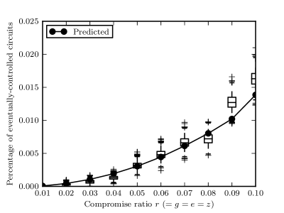
Figure 3. Comparison of analytic model and simulation. The boxes show the interquartile range and median value of the percentage of eventually-controlled circuits. See Appendix A for details.

Returning to the choice of $K$, it turns out that the value (in the range $[2,120]$) has little impact on the effectiveness of the attacker as predicted by the analytic model. The plots corresponding to Figures 1 and 2 are almost unchanged when we set $K=2$; the greatest change is in Figure 1(a), which has the same general contours, but starting with the lowest contour at $.01$ and the highest at $.06$. We might expect that the assumption in the model that circuits only fail because they are killed by the attacker to have more impact with lower values of $K$, since now it seems much more likely that the client would give up before the attacker could control a circuit. This is indeed the case; with $K=2$ the analytic model consistently over-estimates the effectiveness of the attack as implemented in simulation. However, the over-estimation is by a relatively small amount. Analyzing the simulated model with $K=120$, we also see that almost all attempts to build a successful circuit (controlled or not) produce one in $\leq 15$ attempts. Comparing the analytic model to simulation with $K=15$ yields a comparison very close to that shown in Figure 3.

3.3. How much is enough?

It is natural to ask at this point whether any version of the attack is “effective.” In other words: how high must the eventual control probability be for the attack to be considered to be a success? We do not give a specific answer to this question, because it seems that it depends on the goals of the attacker, but we can consider a couple of scenarios.

Suppose a “script-kiddie” just wishes to make some connections between clients and servers, uninterested in the specific identity of either. Then practically any eventual-control probability will do the job. In this case, of course, a passive attack is the route to take.

Suppose a crime-fighting unit or a repressive regime wishes to identify some (initially unknown) users of a specific service. At first blush, it is not clear that denial-of-service is of any great help here, because the users are likely to have no compromised guard nodes; though such users will have a harder time connecting to the service, they will be no more easily identified. But if the goal is to make high-profile “examples” of just a few users, then even a modest success rate could be sufficient, provided it is high enough to identify users within the regime’s jurisdiction. We address the scenario of deploying denial-of-service against a targeted individual in Section 6; such an attacker is likely to have more global resources at her disposal than we are considering here.

4. Detecting the Attack

In this section we show how to detect a DoS attack as described in the previous section. Briefly, the detection algorithm makes $O(n)$ probes of the network, where a probe consists of setting up a circuit and passing data through it. By analyzing the successful and failed probes, we can identify nodes involved in such an attack if they exist. We make the following assumptions about the Tor network and the attacker:

1. The length of the paths used by the Tor implementation under attack is fixed independent of (and strictly less than) $n$ and that paths consist of distinct nodes.

2. The attacker is described by $(p_{\mathrm{kill}},p_{\mathrm{permit}})=(1.0,1.0)$ (the other parameters are unknown).

3. The number of compromised nodes is at least $2$ but less than $n$. Both bounds are reasonable, since at least two compromised nodes are required to perform the underlying traffic confirmation attack on typical circuits, and an anonymity network composed entirely of compromised nodes is of no value to an honest user. We address this assumption further after the proof of the theorem.

4. The only reason a probe fails (i.e., the circuit setup fails or the circuit dies while data is being passed through it) is because it is killed by an attacker on the circuit. Of course, this ignores the fact that honest nodes may also fail, whether due to traffic overload, intentional shutdown, etc.; we discuss how to handle this after the proof of the theorem.

Theorem 4.1.

Under the above assumptions we can detect all of the compromised nodes of the Tor network in $O(n)$ probes. For the case of paths of length $3$ the number of probes required is at most $3n$.

Proof.

Let $k$ be the length of the paths used by the Tor implementation under consideration. We denote the probe consisting of the path of length $k$ starting with $u_{1}$ and ending with $u_{k}$ with edges between $u_{i}$ and $u_{i+1}$ for $i=1,\ldots,u_{k-1}$ by $(u_{1},\ldots,u_{k})$. We say a probe succeeds if the circuit is not killed, otherwise it fails.

Choose a set $X=\{x_{1},\ldots,x_{k-1}\}$ of $k-1$ distinct nodes, arbitrarily. Perform the following set of probes: $(x_{1},y,x_{2},\ldots,x_{k-1})$ for each $y$ not in $X$. One of three cases results.

Case 1: All $n-k+1$ probes succeed

In this case both $x_{1}$ and $x_{k-1}$ must be compromised (if one is, then every probe is compromised but uncontrolled; if neither is, then at least one probe is compromised but uncontrolled; in either case, not all probes succeed). For any node $y\notin X$, $y$ is compromised if and only if the probe $(x_{1},\ldots,x_{k-1},y)$ is successful. To test nodes in $X$, fix any $x\notin X$ and consider probes of the form $(x_{1},\dots,x_{i-1},x,x_{i+1},\dots,x_{k-1},x_{i})$ for each $x_{i}\in X$, $2\leq i<k-1$; again, $x_{i}$ is compromised if and only if this probe is successful.

Case 2: Among the $n-k+1$ probes, at least one succeeds and at least one fails

If either endpoint were compromised, then either all probes would succeed (if the other endpoint were compromised) or all probes would fail (if the other endpoint were uncompromised). Thus neither endpoint is compromised. But then if any of $x_{2},\dots,x_{k-2}$ were compromised every probe would fail. Thus in this case all of the nodes in $X$ are uncompromised, any $y$ for which the probe failed is compromised, and any $y$ for which the probe succeeded is uncompromised.

Case 3: All $n-k+1$ probes fail

In this case we can conclude that either all nodes in $X$ are uncompromised and all nodes not in $X$ are compromised, or at least one of the nodes in $X$ is compromised (otherwise all nodes in $X$ and some node not in $X$ are uncompromised, so at least one probe succeeds). For each pair of nodes $x_{i},x_{j}\in X$ consider probes of length $k$ of the form $(x_{i},y,\dots,x_{j})$, where positions $3$ through $k-1$ consist of $X\setminus\{x_{i},x_{j}\}$ in an arbitrary fixed order and $y$ ranges over nodes not in $X$. Suppose that for some pair $x_{i},x_{j}\in X$ all probes succeed. This second round of probes is the same as the first, but with a different arrangement of the nodes in $X$. Thus the same reasoning as in Case 1 lets us conclude that $x_{i}$ and $x_{j}$ are compromised and we proceed as in that case to determine the status of the remaining nodes. Otherwise, for each pair $x_{i},x_{j}\in X$ there is $y\notin X$ such that the probe $(x_{i},y,\dots,x_{j})$ fails. In this case, if there is at least one uncompromised node in $X$, then there is exactly one uncompromised node in $X$. Now we consider probes of length $k$ of the form $(x,\dots,y)$, where $x\in X$, positions $2$ through $k-1$ consist of $X\setminus\{x\}$ in an arbitrary fixed order, and $y$ ranges over nodes not in $X$. Suppose every probe of the form $(x,\dots,y)$ fails. If there were exactly one compromised node in $X$, then necessarily every node not in $X$ is uncompromised, which means that there is exactly one compromised node in the entire network, violating our assumption that there are at least two such nodes. Thus we conclude that if all probes $(x,\dots,y)$ fail, then no nodes in $X$ are compromised and all nodes not in $X$ are compromised. Otherwise there are $x\in X$ and $y\notin X$ such that $(x,\dots,y)$ succeeds. Suppose $x$ were not compromised. Then there would be a compromised node in $X\setminus\{x\}$ or $y$ would be compromised; in either case the probe $(x,\dots,y)$ would fail, a contradiction. So $x$ is compromised and hence $x$ is the only compromised node in $X$. Furthermore, the compromised nodes not in $X$ are precisely those $y$ such that the probe $(x,\dots,y)$ succeeds.

Analysis

The worst case number of probes occurs in Case $3$ in which we do at most $({k-1\choose 2}+k-1)(n-k+1)$ probes beyond the initial $n-k+1$ probes that define the cases. As $k$ is assumed to be fixed independent of $n$ this is clearly $O(n)$. For the case $k=3$ (the default for Tor), we notice that the initial set of probes and the first set of probes in Case $3$ are the same, so we conclude that the total number of probes is $\leq 3n$. ∎

What happens if we apply this algorithm, but there are no compromised nodes? Case 1 of the proof applies, and since every probe described in that case would succeed, we would conclude that every relay in the network is compromised. In fact, the same applies if all nodes are compromised. At this point, presumably a human would step in to determine whether it is more likely that no relays are compromised or the entire network is, and take action accordingly.

A concern with this detection algorithm is that if $x_{1}$ is a compromised relay, then the attacker likely notices that she is the entry guard in a sequence of circuits in which the middle nodes traverse the entire network. Presumably the attacker stops killing circuits, so we follow Case 2; we end up concluding that $x_{1}$ is uncompromised, and a further side-effect is that $x_{1}$ effectively ends up framing other (uncompromised) nodes. But how likely is this scenario? The probability that $x_{1}$ is compromised is the fraction of compromised guard nodes (by number, not bandwidth). Assuming some degree of human intervention, and assuming that a relay must be identified as compromised multiple times, the attacker escapes detection only if we repeatedly choose her nodes in the set $X$, which happens with low probability.

Now we discuss how to handle the situation in which a probe may fail for reasons unrelated to an attacker (e.g., an honest node may fail, or there may be a transient network failure on one of the links). The problem is that the detection algorithm cannot tell what the source of the failure is. We now define a probe to consist of $r$ attempts to create the specified circuit, where $r$ depends on the failure rate of circuits (compromised or not) and the probability of error in the algorithm we find acceptable. We report that the probe fails if all $r$ of the attempts fail, and otherwise that it succeeds.

We say that a probe is wrong if it fails but either the circuit is uncompromised or it is controlled. Since $(p_{\mathrm{kill}},p_{\mathrm{permit}})=(1.0,1.0)$, a probe consisting of $r$ independent trials can be wrong only if (a) an honest circuit fails $r$ times in a row or (b) a circuit with both end points compromised fails $r$ times in a row. Assume that any given circuit fails due to unreliable nodes or edges with probability $f$. Then, under the independence assumption, (a) or (b) occur with probability at most $f^{r}$, i.e., the probability that a probe consisting of $r$ independent trials is correct is at least $1-f^{r}$. If the algorithm performs $m$ such probes (i.e., probes $m$ circuits overall) the probability they are all correct is greater than $(1-f^{r})^{m}$. Assume we require that our algorithm correctly identifies all nodes as either honest or compromised with probability at least $1-\epsilon$. Then it is easy to see (using standard approximations) that choosing

$$r>\frac{\ln\ln(\frac{1}{1-\epsilon})-\ln m}{\ln f}$$

is sufficient.

We can use our replay data to gain some insight into an appropriate value for $f$. In Figure 4, we show the failure rate for circuit construction. For each trial we constructed a number of circuits by choosing three relays at random (respecting Guard and Exit flags as appropriate) and declaring the circuit a success if all three relays were successfully probed, and a failure otherwise. We choose the relays uniformly at random (i.e., without bandwidth-weighting), because the detection algorithm does not use bandwidth weighting to construct its circuits. For the purpose of choosing a lower bound on $r$, it suffices to find a reasonable upper bound on $f$; from our data, taking $f=.45$ suffices. If we also take $m=7500$ (the worst-case number of probes for a $2500$-node Tor network) and $\epsilon=.0004$ (so that we expect less than one misidentification) we see that $r=21$ is sufficient. So on the deployed network, this modified algorithm would perform $\leq 3rn=63n$ probes.

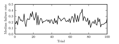
Figure 4. Median circuit failure rates from replay data. For details, see Appendix A.

Of course, we require that the above repeated attempts be independent which is unlikely to be the case. But by spreading the repetitions out over time we can increase our confidence that observed failures are not caused by randomly-occurring transient network failures, bandwidth limits on relays, etc.

5. Detection in Practice

5.1. A “bad-relay, good-relay” detection algorithm

The detection algorithm described in Section 4 along with the measurements made above provide a reasonably practical method for detecting the DoS attack in progress. We can handle non-naive attackers and reduce the number of probes of the network significantly if we are willing to accept probabilistic detection and assume the existence of a single honest router under our control. This single honest router is a trustworthy guard node Wright et al. (2003). This trust is important: Borisov et al. (2007) note that the use of (untrusted) guard nodes in general may make the adversary more powerful when performing the predecessor attack Wright et al. (2002), but the assumption of a trusted guard node avoids this problem entirely. By “trusted” we mean that the node itself is not under the control of an attacker. This can be arranged by installing one’s own router and using it as the guard node. The adversary must not be able to distinguish this node from other guard nodes on the network, for otherwise she can choose to not attack connections from the trusted node and remain hidden. Although this assumption is unrealistic with respect to a global adversary that can observe all network traffic (because of the very specific traffic patterns coming out of this node), we are assuming that our adversary is local. Furthermore, we are not arguing that every user should have a trusted guard node, but rather just the user or organization running the detection algorithm we describe here (see Section 7 for more discussion).

The simplified detection algorithm works as follows. First, query the Tor directory servers for a list of exit nodes, possibly restricted by requiring some degree of stability according to the various flags associated to each node. Call this list of nodes the candidate exits. Then, repeat the following steps $l$ times for some value of $l$: for each candidate node, create a circuit where the first node is our trusted node and the second is a candidate. Retrieve a file through this circuit, and log the results. Each such test either succeeds completely, or fails at some point, either during circuit creation or other initialization, or during the retrieval itself. Either failure mode could be the result of a natural failure (e.g., network outages, overloaded nodes), or an attacker implementing the DoS attack. A candidate node with a high failure rate is a suspect exit; this failure rate can be tuned with the usual trade-off between false positives and negatives. Repeat an analogous process to create a list of suspect guard nodes; this time the circuit starts at a guard node chosen at random and exits at our trusted node.

Once the lists of suspect guards and exits are generated, the following steps are repeated $l^{\prime}$ times for an appropriately chosen $l^{\prime}$. Each possible pairing of a suspect guard and suspect exit is used to create a circuit of length two. As above, the circuits thus created are used to perform a retrieval, and the successes and failures are logged. In this set of trials, we are looking for paths with low failure rates over the $l^{\prime}$ trials. Nodes on such paths could be under control of the adversary, and are termed guilty.

This detection algorithm performs at most $ln+l^{\prime}n^{2}$ probes of the network. From the simulation results described next, we can take $l=l^{\prime}\leq 15$. Furthermore, the number of suspects is usually much less than $n$; we will see that it is typically about $n/10$. Finally, we have also determined that instead of considering every pairing of a suspect guard and exit, for each suspect we can choose $20$ relays of the complementary type at random and consider the $20$ corresponding pairs. Putting all this together results in a detection algorithm that performs $\leq 17n$ probes of the network, as compared to the $63n$ probes required by the algorithm of the previous section.

5.2. The algorithm in simulation

We implement this detection algorithm against our simulation of the denial-of-service attack described in Section 3.2. Our implementation is as follows:

1. Mark some number of relays as attackers as described in Section 3.2, choosing as many guard-exit relays as possible.

2. Choose a suspect cutoff rate ($\mathit{scr}$) and a guilty cutoff rate ($\mathit{gcr}$).

3. Perform suspect-node detection:

   1. Choose $l$ equally-spaced trials $t_{s,0},\dotsc,t_{s,l-1}$ for some $l$.

   2. For each relay $R$ with either the Guard or Exit flag set in at least one of the $t_{s,i}$ and such that $\ell_{R}(t_{s,i})\not=-1$ for some $i$, define the failure rate for $R$ to be $1-m/n$, where $m$ is the number of times $\ell_{R}(t_{s,i})=1$ and $n$ is the number of times $\ell_{R}(t_{s,i})\geq 0$. Mark $R$ as a suspect if its failure rate is $\geq\mathit{scr}$.

4. Perform guilty-node detection:

   1. Choose $l^{\prime}$ equally-spaced trials $t_{g,0},\dotsc,t_{g,l^{\prime}-1}$ for some $l^{\prime}$ with $t_{s,l-1}<t_{g,0}$.

   2. For each pair of suspect relays $R$ and $R^{\prime}$ such that $R$ is a guard and $R^{\prime}$ an exit in trial $0$, define the failure rate for the pair $(R,R^{\prime})$ to be $1-m/n$, where $m$ is the number of times both relays are in the consensus and $(R,R^{\prime})$ is successful and $n$ is the number of times both relays are in the consensus. A pair is successful if both relays were successfully probed and $(R,M,R^{\prime})$ is not killed by the attacker, where $M$ is a relay that we control (and hence is always up and not an attacker). The pair $(R,R^{\prime})$ is guilty if its failure rate is $\leq\mathit{gcr}$.

   3. Label the relay $R$ as guilty if there is a guilty pair $(R,R^{\prime})$ or $(R^{\prime},R)$ for some $R^{\prime}$.

We choose different trials for suspect and guilty node detection, because the latter must be started after the former has completed. We choose a starting trial so that all suspect and guilty node detection trials can be completed before the end of the replay data. In our implementation, we take $t_{s,i+1}=t_{s,i}+1$, $t_{g,i+1}=t_{g,i}$, and $t_{g,0}=t_{s,l-1}+1$ and choose $t_{s,0}$ so that $t_{s,0}+l+l^{\prime}$ is less than the total number of trials in our data.

In either phase, a false positive is an honest relay that is labeled a suspect or guilty, and a false negative is a compromised relay that is not so labeled. A higher suspect cutoff rate reduces the number of relays marked as suspects, whereas a higher guilty cutoff rate increases the number of relays marked as guilty. Therefore increasing $\mathit{scr}$ decreases the false-positive rate and increases the false-negative rate, whereas increasing $\mathit{gcr}$ increases the false-positive rate and decreases the false-negative rate. If we assume that the attacker operates naively (i.e., $(p_{\mathrm{kill}},p_{\mathrm{permit}})=(1.0,1.0)$) and that her relays are perfect (always in the consensus and never fail), then setting $\mathit{scr}=1.0$ will minimize the number of false positives without admitting any false negatives. This is because compromised relays will always fail, whereas an innocent relay has to succeed just once to not be marked as a suspect. Perfection seems unlikely, so instead we will consider an attacker whose relays are reliable, in that they are simultaneously in the top $75$% of relays ranked by bandwidth and by number of times in the consensus (in our simulations, the attacker compromises reliable relays starting at the $90$-th percentile of bandwidth). Although this does not seem like a strong restriction for reliability, in fact it turns out that we have no false-negative suspects if the attacker meets this condition even when $\mathit{scr}=1.0$. Thus the attacker must either run relays that are rarely in the consensus (of dubious value for the attacker) or our algorithm will label all attacking relays as suspects.

There will still be false positives in the suspect labeling; these are relays that are honest but unreliable, and hence have a high “natural” failure rate. These will be filtered out during guilty-node detection, which we can see as follows. Let $R$ be such an unreliable honest relay. Consider any pair of suspects $(R,R^{\prime})$. Since $R$ is unreliable, this pair will almost never succeed, either because $R$ is out of the consensus, or $R$ is in the consensus but fails (it does not matter whether $R^{\prime}$ is honest or compromised). Thus $(R,R^{\prime})$ has a high failure rate, so is unlikely to be labeled as guilty. Since this is the case for every pair $(R,R^{\prime})$ or $(R^{\prime},R)$, $R$ itself is unlikely to be labeled as guilty. Thus for a perfect attacker, setting $\mathit{gcr}=0.0$ will ensure that we have no false negatives during guilt detection while minimizing the number of false positives. It turns out that this holds also for a merely reliable attacker, presumably because her relays are in the consensus frequently enough that they will participate in at least one circuit with average failure-rate $0.0$.

It is still possible to have false-positives when detecting guilty relays. For example, such relays could be in the consensus at least once during suspect-detection and fail in every such trial, but then in the consensus at least once during guilt-detection and succeed in every such trial. There are such relays in our replay data. In Figure 5 we show the false-positive rate as a function of the number of trials during suspect and guilt detection. As we can see, there is a slight increase in the rate as the number of trials increases. This is because a false-positive is typically an unreliable relay; increasing the number of trials during suspect detection gives such a relay a chance to be seen by the detection algorithm, but since it is likely to fail, it will be labeled as a suspect. Likewise, during guilt detection, it is more likely to be seen with more trials; if it is only in the consensus once, then it only needs to be part of a single successful circuit to be labeled guilty, as the failure rate of that circuit is computed with respect to the number of times that circuit can be formed.

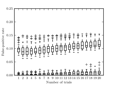
Figure 5. False-positive rates for suspect and guilty detection with the reliable naive attacker. The suspect rates are in the $10$–$15$% range and the guilty rates are in the $0$–$1$% range. For details, see Appendix A.

Next we consider a non-naive attacker. As an example, consider an attacker with $(p_{\mathrm{kill}},p_{\mathrm{permit}})=(0.8,0.8)$ (so, as per the results in Section 3.1, compromises about $70$–$80$% as many circuits as the naive attacker). Setting $\mathit{scr}=1.0$ leads to an unacceptably high false negative rate during suspect detection ($.50$–$1.0$, increasing as we increase the number of trials), as the attacker will rarely have a perfect success rate, even if she only has reliable relays. The false-positive rate is comparable to that when detecting the naive attacker, as the attacker strategy does not affect the behavior of non-attacking relays during suspect detection. Figure 6 shows the false-positive and -negative rates as $\mathit{scr}$ is varied (in all such figures, solid lines indicate false-positive rates, dashed lines false-negative rates). As we can see, provided we are willing to run suspect detection for $10$ trials, we can take $\mathit{scr}=.4$ and have no false-negatives with an acceptable false-positive rate.

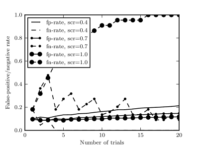
Figure 6. False-positive and -negative rates for suspect detection with the reliable tuned attacker with $(p_{\mathrm{kill}},p_{\mathrm{permit}})=(.8,.8)$. See Appendix A for details, including an explanation of the “zig-zag pattern” for $\mathit{scr}=0.7$.

Figure 7 shows the false-positive and -negative rates for guilty detection as $\mathit{gcr}$ is varied, keeping $\mathit{scr}=.4$. Again we see that we can reduce the false-negative rate to $0.0$, while maintaining a false-positive rate of approximately $2.5$% by running the guilty detection phase for $8$–$10$ trials and taking $\mathit{gcr}=.30$.

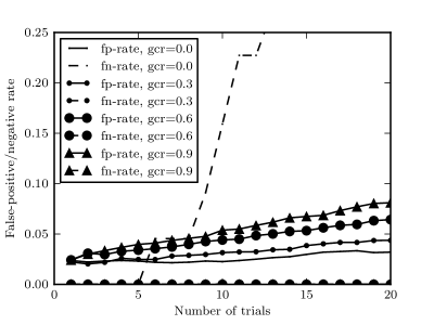
Figure 7. False-positive and -negative rates for guilty detection with the reliable tuned attacker with $(p_{\mathrm{kill}},p_{\mathrm{permit}})=(.8,.8)$. See Appendix A for details.

Finally we consider how well our detection algorithm works as the attacker reduces her kill probability from $1.0$ (the naive attacker) to $0.0$ (the passive attacker), keeping her permit probability at $1.0$. Of course, if $p_{\mathrm{kill}}=0.0$, then the attacker cannot be detected; our interest here is how quickly our algorithm loses effectiveness. Figure 8 shows the suspect false-positive and -negative rates for various values of $\mathit{scr}$; here we have run suspect detection for $15$ trials.

Figure 8. False-negative rates for suspect detection with the reliable attacker with varying kill probabilities and $\mathit{scr}$ values. See Appendix A for details.

As we can see, even if the attacker lowers her kill probability to $.5$ in order to escape detection, we will still have a nearly $0$% false-negative rate during suspect detection, provided we lower $\mathit{scr}$ to $.25$. Of course, lowering $\mathit{scr}$ increases the false-positive rate; in this case, lowering to $.25$ from $1.0$ increases the false-positive rate from about $10$% to about $25$% (this is independent of the attacker’s kill probability, since this does not affect the behavior of non-attackers during suspect detection). This rather high false-positive rate is only an issue if it persists through guilt detection. In Figure 9 we show the false-positive and -negative rates for guilt detection as $\mathit{gcr}$ and the kill probability are varied, where we fix $\mathit{scr}$ at $.25$ and run both suspect and guilt detection for $15$ trials.

Figure 9. False-negative rates for guilty detection with the reliable attacker with varying kill probabilities and $\mathit{gcr}$ values. See Appendix A for details.

Clearly, just about any value of $\mathit{gcr}>0.0$ suffices to reduce the false-negative rate to essentially $0$%, even when the attacker’s kill-probability is $.5$. And provided $\mathit{gcr}<1.0$, the false-positive rate is about $5$%. This seems like a reasonable compromise if the primary goal is to identify compromised relays.

5.3. How good is good enough?

Just as we can ask how effective the denial-of-service attack must be, we can also ask how effective any detection algorithm must be. For example, is a false-positive rate of $5$% acceptable? Again, we do not answer this directly, because this seems to be more of a matter for policy (of course, if the false-positive rate were $90$%, the policy would be easy to settle). We assume that any automated algorithm would really flag “guilty” relays as being relays that deserve further inspection. Probably such inspection would be carried out by humans. The goal of algorithms such as those presented here is to reduce the workload of humans to a manageable level by clearing many relays of suspicion automatically.

6. Variants of the attack

The attacker we have described in Section 2, and on which our detection algorithms are based, kills circuits unconditionally according to the parameters $p_{\mathrm{kill}}$ and $p_{\mathrm{permit}}$. However, an attacker may be interested in a contextual attack, for example only attacking connections to particular hosts or traffic of a certain type. Our analytic model and detection algorithms handle contextual attacks more-or-less well depending on the specifics of the context.

On one end of the spectrum are contexts in which circuit membership can be determined by a relay in any position on the circuit. An example such context is bulk-download traffic. In this case, $p_{\mathrm{kill}}$ and $p_{\mathrm{permit}}$ are the probabilities of killing and permitting circuits that satisfy the context, respectively. The analytic model is unchanged. The only change to the detection algorithm is what constitutes a “probe” of a relay; now it is a circuit that satisfies the context.

Somewhat more challenging are contexts in which circuit membership can only be determined by relays in certain positions. An example is circuits that connect to a specific host; only the exit relay can determine whether the context is satisfied or not. This means that if a guard or middle node determines that it is the only attacker node in the circuit, it does not have enough information to determine whether the circuit satisfies the attack context. Our analytic model can be adapted to handle this attacker by adjusting the calculation of $u_{j}(C)$, the probability that the attempt to build circuit $C$ is unsuccessful when the client has $j$ attacker nodes in his guard node list. Recall that

$$u_{j}(C)=(1-p_{\mathrm{permit}})\cdot\Pr[\text{$C$ controlled}]+p_{\mathrm{kill}}\cdot\Pr[\text{$C$ compr., uncontr.}].$$

What we need to do is to define two kill probabilities: $p_{\mathrm{kill,aware}}$ and $p_{\mathrm{kill,unaware}}$. The former is the kill probability for relays that can determine whether or not the context is satisfied; the latter is for relays that cannot. We can then rewrite the term $p_{\mathrm{kill}}\cdot\Pr[\text{$C$ compr., uncontr.}]$ to take into account both kinds of relays. For the example at hand, this term would be

$$p_{\mathrm{kill,aware}}\Bigl{(}1-\frac{j}{3}\Bigr{)}e^{*}+p_{\mathrm{kill,unaware}}\left(\frac{j}{3}\Bigl{(}1-e^{*}\Bigr{)}+\Bigl{(}1-\frac{j}{3}\Bigr{)}(1-e^{*})m\right).$$

Note that we only need one value for $p_{\mathrm{permit}}$, because if the relays can communicate enough to determine that they are all on the same circuit, then presumably any context-aware relay can convey the context information to the other relays as well. How the “bad-relay, good-relay” detection algorithm fares depends on the relation between $p_{\mathrm{kill,aware}}$ and $p_{\mathrm{kill,unaware}}$. If they are equal, then no change is needed (this is unsurprising, since in this case, the analytic model is also unchanged). But suppose that $p_{\mathrm{kill,unaware}}=0.0$—i.e., an uncontrolled circuit is only killed by an exit relay that observes a connection to the desired host. As described, the first phase of our detection algorithm will have an unacceptable false-negative rate for guards, as they will never kill circuits. It is possible to adapt the algorithm so that all guards are initially labeled as suspects. This increases the cost of the second phase. However, our preliminary experiments indicate that the false-positive and -negative rates for guilt detection are essentially unchanged from those shown in Figure 7. And there is a trade-off for the attacker here. By setting $p_{\mathrm{kill,unaware}}=0.0$, her guards are not suspiciously killing circuits which, in all likelihood, are not even connecting to the targeted endpoint, and this makes our detection algorithm more time-consuming to run. On the other hand, her attack is less effective: our analytic model predicts that she eventually controls about half as many circuits as for the context-independent attack.

An attack targeted at an individual user is much more difficult for our model and detection algorithms. It is unlikely that such an attack would be launched using only relays; it seems much more likely that the attacker controls the user’s ISP and performs denial-of-service in order to control the exit relay. There is no need to control the entry node in this case, as the ISP can view the traffic between the client and entry relay, and that is sufficient. Obviously a centralized authority running our detection algorithm would not see the attack, since it would not be attacked at all. And the ISP could easily see if the individual user were running the algorithm and react accordingly. This highlights the restrictions of the locality assumption of Section 2: we consider denial-of-service attacks that are run from individual Tor relays, not from more powerful attackers who may have more global resources (such as an ISP). We also note that such an attacker might have sufficiently global resources as to be able to launch a purely passive (and hence undetectable) attack using timing analysis techniques such as those described by Murdoch and Zieliński (2007).

In order to reduce the effectiveness of the detection algorithms, an attacker may “frame” honest nodes, under the reasonable assumption that the information content provided by a detection algorithm that produces too many false positives would be too low to be useful. One approach is to kill circuits in an attempt to frame the honest nodes that are on those circuits, but it is not clear that such framing would be effective with the “bad-relay, good-relay” algorithm. In the first phase (suspect detection), only one “wild” node is probed at a time; thus no framing is possible in this phase, and the only false positives are unreliable relays. In the second phase (guilt detection), relays are paired up, and so an attacker might try to frame honest nodes. However, in this phase, a relay is labeled as guilty if it is “too reliable;” since the only honest nodes to make it into this phase are unreliable, and nothing an attacker can do will make them more reliable, it seems difficult to frame any nodes during this phase either. Another approach is to employ denial-of-service attacks to flood an honest relay with traffic, thereby making it a suspect in the first phase of the detection, then stopping the denial-of-service in order to make it guilty in the second. This would require the attacker to know when the detection algorithm is being run, and it is unclear whether one can reasonably defend against an attacker with this level of knowledge.

7. Running the detection algorithms

The algorithms we have proposed here are not intended to be run by individual Tor users (in contrast to the algorithm described by Das and Borisov (2011)). Thus there is legitimate concern as to how these algorithms can be employed in a way that does not fundamentally alter the decentralized nature of Tor. This decentralization is important. If it is known that the detection algorithms are run by a small, specific set of relays, then the attacker can easily avoid detection by simply permitting connections to/from those relays. It would be very interesting to see if a distributed version of these algorithms could be implemented. One possible version would have a large percentage of relays involved in running the detection algorithm, with each relay testing a small portion of the network. Relays would then vote on the results in a manner analogous to how the directory authorities currently vote on flags, etc.

A certain amount of centralization is almost certainly lost though in the final stages. It is problematic at best to allow a fully automated process to block operators from participating in Tor. If a group of relays is deemed by these algorithms to be launching DoS attacks, it seems almost necessary that humans ultimately step in to determine an appropriate course of action.

8. Related work

The arms race between attackers and defenders in anonymity systems has a long history. System designers aim to prevent attacks, or failing that, to detect and respond to them. In turn, attackers attempt to evade or bypass prevention and detection mechanisms. Here, we briefly survey some related work in this arms race.

The MorphMix system Rennhard and Plattner (2002), like Tor, is a peer-to-peer system for low-latency anonymous communication on the Internet. The system’s design includes a collusion detection mechanism. Later, Tabriz and Borisov (2006) showed that local knowledge of the network does not suffice to detect colluding adversaries.

Danezis and Sassaman (2003) propose a detection algorithm for active attacks in mixes, based upon self-addressed heartbeat messages sent through the mix itself. This algorithm is concerned with an $(n-1)$ attack, where an attacker floods an honest node with fake messages to enable the linking of the sender and receiver of a single message; a heartbeat is used to attempt detection of such attacks. The heartbeat mechanism has some parallels to our probing mechanisms, though the attacker models are quite different.

Murdoch (2006; 2007) examines the use and detection of various covert channels in attacks on anonymity systems. The types of attack algorithms and corresponding detection mechanisms again illustrate the arms race, though they do not map to the attacker model we examine.

Das and Borisov (2011) propose a detection algorithm intended to be used by individual Tor users in order to avoid circuits compromised by a DoS attacker; this work is the closest to ours. The algorithm itself is similar to our “bad relay-good relay” detection algorithm (though their algorithm might be described as “good relay-bad relay”). Their goal is to allow clients to identify (potentially) compromised circuits over a short timeframe in order to avoid using them, rather than to identify specific nodes implementing a DoS attack over a longer timeframe. Their approach can be used to mitigate the risk to a user from an ISP-level attacker which, as we discuss in Section 6, our algorithm cannot do (although as we also note there, such an attacker might very well gain enough information from a passive attack). The cost of running their algorithm (in terms of number of circuits created) appears lower than that of our algorithms. However, it is not clear that the overhead on the entire network would actually be lower if all clients were to implement their algorithm.

9. Conclusion

The denial of service attack on Tor-like networks is potentially quite powerful, allowing an adversary to break the anonymity of users at a rate much higher than when passively listening. We have provided a careful analysis of the parameters that define such an attack, as well as an analytic model of the attacker’s effectiveness. We have tested this model against a simulation based on replaying data collected from the deployed Tor network and seen that it is accurate. We have also shown that the power of the denial-of-service attack comes at a price by giving two algorithms that detect any such attacker by constructing a number of circuits that is linear in the number of relays in the network. One such algorithm is deterministic and proved correct given a set of assumptions about the network and attacker, and the other probabilistic and shown to be effective using our replay simulation technique. We finish by discussing how these algorithms fare in the face of attackers who deviate from our model.

Appendix A About the data

All of the data described in this paper, as well as the programs used to collect and analyze it, are publicly available at Wesleyan University’s WesScholar site at http://wesscholar.wesleyan.edu/compfacpub, in the section for this paper. When specific numbers are indicated, they refer to data collected approximately $10$–$11$ June 2011 (timestamps are included in the data). This dataset consists of $100$ trials. Following are some notes on how specific figures were produced:

Figure 3 (Comparison of theoretical model to simulation)

For each $r\in\{.01,.02,\dots,.10\}$, relays in the replay data were compromised according to the algorithm described in Section 3.1 to reach the target goal of $g=e=r$. Then $10,000$ circuits were constructed and $1,000$ bootstraps are performed. Each bootstrap consists of selecting $10,000$ circuits from the population, sampling with replacement, and recording the percentage of selected circuits that are controlled by the attacker. The median and interquartile range of the $1,000$ bootstraps is shown. Then the analytically-predicted value is computed, using the actual guard, exit, and guard-exit compromise ratios and the actual values of $\gamma$, $\eta$, and $\zeta$ as in the collected data.

Figure 4 (Circuit construction failure rate)

For each trial in the replay data, we constructed $100$ circuits and noted whether each was successful or not. We then sampled these circuits with replacement $100$ times and noted the proportion of failed circuits. We do the sampling $10$ times per trial and show the median failure rate.

Figure 5 (Suspect and guilty false-positive rates for the reliable naive attacker)

For each number of trials $n$, we run the suspect detection phase $100$ times. Each time we choose a starting trial at random, run the algorithm over $n$ trials, and record the false-positive rate. We display the median rate and the inter-quartile ranges. Taking $5$ trials as our best number of trials for suspect detection, for each $n$ we run the suspect and guilty detection phases together $100$ times. Each time we choose a starting trial at random, run the suspect phase for $5$ trials, the guilty phase for $n$ trials, and record the false-positive rate for guilt detection. We display the median rate and inter-quartile ranges.

Figure 6 (False-positive and -negative suspect rates for reliable tuned attacker)

For each number of trials $n$ and value of $\mathit{scr}$, we run the suspect detection phase for $n$ trials with the given value of $\mathit{scr}$. Then we compute the false-positive and -negative rates for suspect detection. This is repeated $100$ times, each time choosing a starting trial at random. We plot the median false-positive and false-negative rate for each combination of $n$ and $\mathit{scr}$. The “zig-zag” pattern for the false-negative rate when $\mathit{scr}=0.7$ is an artifact of how the number of trials that a guilty relay must pass to avoid detection changes as the total number of trials increases. This number is $1$ for $1$–$3$ trials; $2$ for $4$–$6$ trials; $3$ for $7$–$9$ trials; etc. If the number of trials to pass to avoid detection does not increase, then the false-negative rate will increase. As $\mathit{scr}$ decreases, the number of trials to pass jumps less frequently, and the false-negative rate is already relatively low, so the pattern is not as obvious at lower values.

Figure 7 (False-positive and -negative guilty rates for reliable tuned attacker)

For each number of trials $n$ and value of $\mathit{gcr}$, we run the suspect detection phase for $10$ trials with $\mathit{scr}=.4$, followed by guilty detection for $n$ trials with the given value of $\mathit{gcr}$. Then we compute the false-positive and -negative rates for guilty detection. This is repeated $100$ times, each time choosing a starting trial at random. We plot the median false-positive and false-negative rate for each combination of $n$ and $\mathit{gcr}$.

Figure 8 (False-negative suspect rates for varying kill probability)

For each value of $\mathit{scr}$ and $p_{\mathrm{kill}}$, suspect detection is run for $15$ trials and the false-negative rate is recorded. This is repeated $100$ times, each time choosing a starting trial at random. The median false-negative rate is plotted for each value.

Figure 9 (False-positive/negative rates for varying kill probability)

For each value of $\mathit{gcr}$ and $p_{\mathrm{kill}}$, suspect detection is run for $15$ trials with $\mathit{scr}$ fixed at $.25$. Then guilt detection is run for $15$ trials with the given value of $\mathit{gcr}$ and the false-positive and -negative rates are recorded. This is repeated $100$ times, each time choosing a starting trial for suspect detection at random. The median rate is plotted for each pair of values.

References

- Bauer et al. [2007] Kevin Bauer, Damon McCoy, Dirk Grunwald, Tadayoshi Kohno, and Douglas Sicker. Low-resource routing attacks against Tor. In Proceedings of the 2007 ACM Workshop on Privacy in Electronic Society (WPES 2007), pages 11–20. Association for Computing Machinery, October 2007.
- Borisov et al. [2007] Nikita Borisov, George Danezis, Prateek Mittal, and Parisa Tabriz. Denial of service or denial of security? How attacks on reliability can compromise anonymity. In Proceedings of the 14th ACM Conference on Computer and Communications Security (CCS 2007), pages 92–102. Association for Computing Machinery, October 2007.