Freeze-out yields of radioactivities in core-collapse supernovae

Abstract

We explore the nucleosynthesis trends from two mechanisms during freeze-out expansions in core-collapse supernovae. The first mechanism is related to the convection and instabilities within homogeneous stellar progenitor matter that is accreted through the supernova shock. The second mechanism is related to the impact of the supersonic wind termination shock (reverse shock) within the tumultuous inner regions of the ejecta above the proto-neutron star. Our results suggest that isotopes in the mass range $12\leqslant A\leqslant 122$ which are produced during the freeze-out expansions may be classified in two families. The isotopes of the first family manifest a common mass fraction evolutionary profile, whose specific shape per isotope depends on the characteristic transition between two equilibrium states (equilibrium state transition) during each type of freeze-out expansion. The first family includes the majority of isotopes in this mass range. The second family is limited to magic nuclei and isotopes in their locality which do not sustain any transition, become nuclear flow hubs, and dominate the final composition. We use exponential and power-law adiabatic profiles to identify dynamic large-scale and small-scale equilibrium patterns among nuclear reactions. A reaction rate sensitivity study identifies those reactions which are crucial to the synthesis of radioactivities in the mass range of interest. In addition, we introduce non-monotonic parameterized profiles to probe the impact of the reverse shock and multi-dimensional explosion asymmetries on nucleosynthesis. Cases are shown where the non-monotonic profiles favor the production of radioactivities. Non-monotonic freeze-out profiles involve longer non-equilibrium nucleosynthesis intervals compared to the exponential and power-law profiles, resulting in mass fraction trends and yield distributions which may not be achieved by the monotonic freeze-out profiles.

1 INTRODUCTION

Despite the progress in core-collapse supernova theory during the past 20 years, the details of a fully self-consistent explosion and the nucleosynthesis are not yet fully understood. Three-dimensional supernova simulations with energy-dependent neutrino transport are necessary to clarify the growth of convective and Rayleigh–Taylor instabilities, the possibility of non-radial, non-axisymmetric instability modes, and the development of local fluid vortices (Janka et al., 2007). Further mixing processes near the proto-neutron star surface that could enhance the neutrino heating behind the shock include doubly diffusive instabilities (Bruenn et al., 2004), neutrino-bubble instabilities (Socrates et al., 2005), and magnetic buoyancy instabilities (Wilson et al., 2005). The neutrino heating results in the outflow of baryonic matter (wind) from the surface of the proto-neutron star (Duncan et al., 1986). This neutrino-driven wind interacts with the more slowly moving, earlier supernova ejecta forming a wind termination shock, which is also termed as reverse shock (Burrows et al., 1995; Janka & Müller, 1995). The position of the reverse shock depends on the wind velocity and the thermodynamic conditions of the supernova ejecta which the wind collides with (Arcones et al., 2007), while its boundary is strongly deformed to a non-spherical shape in multi-dimensional simulations (Arcones & Janka, 2011).

The interaction of the supernova shock with the stellar progenitor layers and the reverse shock with the mass layers above the proto-neutron star results in sudden entropy increases which trigger nucleosynthesis in the ashes of pre-collapse nuclear burning. The expanding material then cools down until nuclear reactions freeze-out. The temperature and density trajectories of the expanding ejecta located initially outside the range of convective and mixing processes are monotonically decreasing. However, certain thermodynamic trajectories may be non-monotonic and can affect the abundances’ evolution in non-trivial ways. Possible factors to result in non-monotonic trajectories include the explosion energetics (Nakamura et al., 2001), explosion asymmetries in multi-dimensional simulations (Nagataki et al., 1997, 1998), rotating progenitors (Fryer & Heger, 2000), double explosion scenaria (Fryer et al., 2006), and the effect of the reverse shock (Arcones et al., 2007; Arcones & Janka, 2011). The yields from non-monotonic trajectories are usually different compared to compositions from monotonic trajectories.

Certain studies have explored the impact of the supernova shock and the reverse shock on nucleosynthesis processes such as the $\alpha$-rich and neutron-rich freeze-out (Woosley & Hoffman, 1992; Witti et al., 1994), the $\nu$$p$-process (Fröhlich et al., 2006; Pruet et al., 2006), the $rp$-process (Wanajo, 2006), and the $r$-process (Takahashi et al., 1994). For the $r$-process specifically, the impact of the reverse shock has been studied under various wind schemes which include subsonic “breeze” solutions with constant pressure boundaries (Terasawa et al., 2002), supersonic winds with fixed asymptotic temperature (Wanajo et al., 2002), and two-phase outflow models (Kuroda et al., 2008), including reverse shock temperature ranges which could trigger the “cold” $r$-process (Wanajo, 2007) or the classical $r$-process (Kratz et al., 2007). However, integrated nucleosynthesis based on those simulations shows that no heavy $r$-process elements can be produced (Arcones & Montes, 2011). In addition, reaction rate sensitivity studies have been performed to constrain uncertainties related to the $p$-process (Rapp et al., 2006), $\nu$$p$-process (Wanajo et al., 2011), freeze-out expansions from nuclear statistical equilibrium (henceforth NSE) or quasi-static equilibrium (henceforth QSE) in The et al. (1998); Hoffman et al. (2010); Magkotsios et al. (2010), and hydrostatic burning (Tur et al., 2010). Sensitivity studies add detail to the understanding of the microscopic mechanisms which drive the related processes, because these mechanisms may not be easily identified for nominal values of the reaction rates or other related parameters.

Yields of radioactivities as inferred from observations and presolar signatures (calcium and aluminum-rich inclusions, inter-planetary dust particles, and stellar grains) add complexity and raise new challenges for the explosion mechanism. Isotopic anomalies in presolar signatures indicate discrepancies between measured or inferred isotopic ratios and current supernova theory. The gamma-ray diffusive emission pattern of $\mathrm{{}^{26}Al}$ indicates that massive stars are its most probable source (Leising & Diehl, 2009; Limongi & Chieffi, 2006b; Tur et al., 2010), given its correlation to $\mathrm{{}^{60}Fe}$ (Timmes et al., 1995; Limongi & Chieffi, 2006a). Yet, the synthesis of $\mathrm{{}^{60}Fe}$ is largely dependent on the reaction rates producing it (Leising & Diehl, 2009). $\mathrm{{}^{41}Ca}$ found in SiC grains is likely to have common origin with $\mathrm{{}^{26}Al}$ (Sahijpal et al., 1998), with a small fraction of $\mathrm{{}^{41}Ca}$ possibly originating from supernova explosions (Nittler et al., 2008). It is argued that $\mathrm{{}^{53}Mn}$ was uniformly distributed in the early solar nebula (Yamashita et al., 2010). Although $\mathrm{{}^{53}Mn}$ is produced in significant amount in core-collapse supernovae, it does not emit $\gamma$-rays which would be easily detectable, but only X-rays which require significant accumulation in the interstellar medium for successful detection (Leising & Diehl, 2009). $\mathrm{{}^{79}Se}$ also lacks a decay scheme by $\gamma$-rays, although its detection in presolar grains is possible. Heavier isotopes such as $\mathrm{{}^{93}Zr}$ (Lugaro et al., 2003), $\mathrm{{}^{92}Nb}$, and $\mathrm{{}^{97}Tc}$ are believed to be produced primarily in asymptotic giant branch (AGB) stars, although we demonstrate cases where they may be produced in significant amounts during supernova explosions.

In this study, we use monotonic adiabatic profiles to quantify nucleosynthesis trends caused by equilibrium patterns among nuclear reactions. In addition, we introduce non-monotonic parameterized expansion profiles to simulate the impact of two mechanisms which may result in non-monotonic evolution for the local temperature and density evolution. The first mechanism involves multi-dimensional effects of the explosion following the passage of the supernova shock through the homogeneous layers of progenitor gas, and the second mechanism involves the impact of the abrupt deceleration by the reverse shock to the supersonic wind originating from the surface of the proto-neutron star. The mechanisms are independent of each other, because a contact discontinuity prevents mixing between the accumulated wind matter and the dense layer of shock-accelerated progenitor gas (Arcones et al., 2007). The non-monotonic profiles result in yield profiles which may not be achieved by the monotonic expansions. These results indicate the importance of multi-dimensional supernova simulations on nucleosynthesis within the tumultuous stellar mass layers. We demonstrate cases where the non-monotonic profiles favor the production of radioactivities, and conclude that under certain circumstances non-monotonic profiles may increase the likelihood of detecting radioactivities in observed supernovae.

Section 2 is a summary of our previous work (Magkotsios et al., 2010). In Section 3 we present the formalism of the parameterized thermodynamic trajectories. Section 4 considers general trends of isotopes in the mass range $12\leqslant A\leqslant 122$ from our exponential and power-law trajectories. Sensitivities to reaction rate values related to the synthesis of radioactivities are discussed in Section 5. The impact of non-monotonic profiles on nucleosynthesis is discussed in Section 6. We conclude our discussion with a summary of our new results in Section 7.

Our nomenclature is based on the following conventions. The temperature of the material is expressed by the pure number $T_{9}=T/(10^{9}\ {\rm K})$. The electron fraction, or the total proton to nucleon ratio is $Y_{e}=\sum_{i}Z_{i}Y_{i}=\sum_{i}{Z_{i}}/{A_{i}}\ X_{i}$. We define “nuclear flow” to mean the instantaneous rate of change of isotope $i$’s molar abundance with time ($dY_{i}/dt$) due to a given nuclear reaction (Iliadis, 2007). For any single reaction linking isotope $i$ with isotope $j$ there is a forward flow, a reverse flow, and a relative net flow $\phi_{i}$=(forward $-$ reverse)/max(forward,reverse) that measures the equilibrium state of the reaction.

2 SYNOPSIS OF PREVIOUS WORK

The current work is a continuation of Magkotsios et al. (2010). We provide a synopsis of key notions and results presented in our previous work which are relevant to our new results. Magkotsios et al. (2010) used two parameterized expansion profiles within a parameter space of peak temperatures, peak densities, and initial electron fraction values, to discuss nucleosynthesis trends related to $\mathrm{{}^{44}Ti}$ and $\mathrm{{}^{56}Ni}$ during freeze-out expansions from core-collapse supernovae. The initial composition was dominated by $\mathrm{{}^{28}Si}$, with neutrons or protons added to configure the value of the initial electron fraction $Y_{e}$. Setting the initial composition in this manner was not restrictive for the largest part of our parameter space. The peak conditions established a large-scale structure composed by nuclear reactions in equilibrium and the mass fractions within this structure were rearranged to their equilibrium values early during the evolution. Large-scale equilibrium structures involve either nuclear statistical equilibrium (NSE), or global quasi-static equilibrium (global QSE). During NSE every reaction within a network is in equilibrium, while a small subset of them may be off equilibrium during QSE. For decreasing temperature and density values during the expansion the large-scale QSE cluster dissolves in multiple small-scale QSE clusters, where each cluster encompasses only a small number of nuclei with similar masses (local QSE). Further decrease in the temperature and density results in the cease of nuclear reactions (freeze-out stage).

Multiple types of freeze-out expansions were identified and discussed within the parameter space used, such as the normal freeze-out (Woosley et al., 1973; Meyer, 1994; Meyer et al., 1998; Hix & Thielemann, 1999), the $\alpha$-rich freeze-out (Woosley et al., 1973), the $\alpha$-rich and proton-rich freeze-out ($\alpha$$p$-rich), the incomplete silicon burning regime,, the photodisintegration regime the $\mathrm{(p,\gamma)}$-leakage regime for $Y_{e}>0.5$, the $\alpha$-rich and neutron-rich freeze-out for $Y_{e}<0.5$ ($\alpha$$n$-rich), and the depletion region of yields which separates the incomplete silicon burning and normal freeze-out regions from the $\alpha$-rich freeze-out (chasm).

Each type of freeze-out is related to distinct transitions between two very different equilibrium states. In this work we refer them as “equilibrium state transitions” and we abbreviate them as EST. These transitions between equilibrium states involve multiple reactions within the QSE cluster which break equilibrium, resulting in changes to the QSE cluster’s size and shape. The scale of the transitions during freeze-out expansions may be global, such as the division of a large QSE cluster encompassing almost every isotope in the network into two large QSE clusters localized within the silicon and iron groups respectively. Alternatively, the scale of the transitions may be local, involving only a small set of nuclear reactions which form small-scale clusters such as equilibrium chains of $\mathrm{(p,\gamma)}$ or $\mathrm{(n,\gamma)}$ reactions interacting with $\alpha$-captures or $\mathrm{(p,n)}$ reactions, respectively. ESTs are entropy driven, where the temperature sets an approximate threshold for a transition, while the density at the threshold temperature determines whether the transition takes place or not. Electron fraction variations, the expansion timescale, and key reaction rates control the local equilibrium patterns which shape the locus of each region.

3 PARAMETERIZED PROFILES

The nucleosynthesis calculations implement mature reaction network solvers (Timmes, 1999; Fryxell et al., 2000) and utilize the 489 and 3304 isotope networks described in Magkotsios et al. (2010). The 489 isotope network has been expanded to 553 isotopes to include a sufficient amount of isotopes near the magic number 50, and is listed in Table 1. The 553 isotope network includes two separate isomers for $\mathrm{{}^{26}Al}$, $\mathrm{{}^{26}Al}$_g for the ground state and $\mathrm{{}^{26}Al}$_m for the first excited metastable state. We use three parameterized profiles to model the freeze-out expansions. All profiles assume that a passing supernova shock wave heats material to a peak temperature $T_{0}$ and compresses the material to a peak density $\rho_{0}$. This material then expands and cools down (freezes out) until the temperature and density are reduced to the extent that nuclear reactions cease.

The first two parameterized profiles involve monotonic temperature and density decrease, following a constant $T^{3}/\rho$ evolution which implies constant radiation entropy in suitable limits. The first profile is the exponential expansion (Hoyle et al., 1964; Fowler & Hoyle, 1964)

$$T(t)=T_{0}\exp(-t/3\tau)\quad\rho(t)=\rho_{0}\exp(-t/\tau)$$ (1)

with a static free-fall timescale for the expanding ejecta

$$\tau=(24\pi G\rho_{0})^{-1/2}\approx 446/\rho_{0}^{1/2}\ {\rm s.}$$ (2)

The exponential profile has been used extensively in the past to explore yield trends and their sensitivity to reaction rates or electron fraction values (Woosley et al., 1973; Woosley & Hoffman, 1992; The et al., 1998; Hoffman et al., 2010; Magkotsios et al., 2010). The second profile is a power-law based on homologous expansion introduced by Magkotsios et al. (2008, 2010)

$$T(t)=\frac{T_{0}}{ct+1}\quad\rho(t)=\frac{\rho_{0}}{(ct+1)^{3}}\enskip,$$ (3)

where the coefficient $c=2$ s^-1 is chosen to mimic trajectories taken from core-collapse simulations.

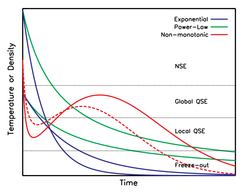
Figure 1: Schematic temperature or density evolution for the exponential, power-law and non-monotonic profiles. Passages through different burning regimes for various peak conditions are indicated. The dashed red curve illustrates the impact of variations to the values of the local extremum points for the same peak conditions.

Figure 1 compares the general properties of the exponential and power-law profiles. For a given initial condition, the power-law evolution is always slower than the exponential one. Moreover, the power-law evolution becomes slower for increasing peak temperature and density values. The differences in these two profiles affect the final yields as material traverses different burning regimes on different timescales. The figure also depicts the NSE, global QSE, local QSE, and final freeze-out burning regimes. The exponential and power-law trajectories are chosen so that they generally bound the temperature and density trajectories of hydrodynamic particles from spherically symmetric and two-dimensional explosion models.

We introduce non-monotonic profiles to simulate possible thermodynamic conditions in the ejecta from different mass layers within the star. Non-monotonic temperature and density evolution may arise due to convection and instabilities following the heating of homogeneous progenitor mass by the supernova shock, or by the termination shock to the supersonic wind within the inner mass layers above the proto-neutron star. Our profiles involve three stages to model such possible effects (Figure 1). During the first stage, the supernova shock rises the temperature and density values of the material traversed, and the material is allowed to expand while it cools and rarefies. During the second stage we introduce a simplified approach to model the effect of multi-dimensional asymmetries to the explosion or the reverse shock within a parameterized expansion profile. This stage involves a contraction phase which rises the temperature and density linearly in time to a local maximum. The third stage involves an exponential freeze-out, because the material is assumed to be part of the ejecta and eventually escape from the star. Contrary to the exponential and power-law cases, no explicit assumption is made about holding $T^{3}/\rho$ constant.

Each temperature and density trajectory has a peak value followed by a local minimum and then a local maximum. The local minimum and maximum values for the case of the reverse shock depend on the wind velocity and the deformed boundary of the shock near the supernova ejecta which the wind collides with (Arcones et al., 2007; Arcones & Janka, 2011). For the case of our parameterized expansion profiles, we choose the local extremum values for temperature and density randomly from a uniform distribution. Each value of a local extremum point is considered to be independent and identically distributed. This is a reasonable approach, because we aim to study the key nucleosynthesis trends within the tumultuous inner layers of the ejecta, and we attempt to simplify the hydrodynamic evolution for this purpose.

The differential equations for the non-monotonic temperature and density trajectories are

$$\frac{dT}{dt} =-T_{0}\exp(-k_{{}_{T}}t)\biggl{[}k_{{}_{T}}b_{{}_{T}}t+\frac{k_{{}_{T}}}{1+a_{{}_{T}}t}+\frac{a_{{}_{T}}}{(1+a_{{}_{T}}t)^{2}}-b_{{}_{T}}\biggr{]}$$ (4)

$$\frac{d\rho}{dt} =-\rho_{0}\exp(-k_{\rho}t)\biggl{[}k_{\rho}b_{\rho}t+\frac{k_{\rho}}{1+a_{\rho}t}+\frac{a_{\rho}}{(1+a_{\rho}t)^{2}}-b_{\rho}\biggr{]}$$ (5)

and their solutions are

$$T(t) =T_{0}\exp(-k_{{}_{T}}t)\biggl{[}\frac{1}{1+a_{{}_{T}}t}+b_{{}_{T}}t\biggr{]}$$ (6)

$$\rho(t) =\rho_{0}\exp(-k_{\rho}t)\biggl{[}\frac{1}{1+a_{\rho}t}+b_{\rho}t\biggr{]}\enskip,$$ (7)

where the parameters $a_{i}$, $b_{i}$ and $k_{i}$ may be chosen to control the local extremum points. For instance, the density minimum is given approximately by $\rho_{min}=\rho_{0}(2\sqrt{a_{\rho}b_{\rho}}-b_{\rho})/a_{\rho}$ at time $t_{min}=(\sqrt{a_{\rho}}-\sqrt{b_{\rho}})/(a_{\rho}\sqrt{b_{\rho}})$, while the maximum is given by $\rho_{max}=\rho_{0}/(e\;k_{\rho})$ at time $t_{max}=1/k_{\rho}$. The red curves of Figure 1 show the profile’s general trends compared to the exponential and power-law expansions. The ascending trajectory is focused on QSE and local equilibrium stages. We ensure that the local maximum for the temperature does not exceed the NSE threshold, otherwise the preceding part of the trajectory would not impact the evolution. The local minimum for the temperature ranges from the freeze-out temperature $T_{9}=0.01$ until the peak temperature. The subsequent local maximum for the temperature ranges from the value of the local minimum until the value $T_{9}=4$. Thus, a non-monotonic evolution is guaranteed without the re-establishment of NSE. The range of the extremum point values for the density profile is less constrained and even monotonic profiles may arise. The minimum spans the range $10^{5}$ g cm^-3 $<\rho_{min}<\rho_{0}$ and the range for the maximum is $10^{6}$ g cm^-3 $<\rho_{max}<10^{9}$ g cm^-3.

4 YIELDS FROM THE EXPONENTIAL AND POWER-LAW PROFILES

The exponential and the power-law expansion profiles used in this work set the basis for quantifying the details of nucleosynthesis mechanisms. Their low computational cost allows the monitoring of large-scale and small-scale equilibrium patterns among nuclear reactions in time, which is a powerful tool for identifying microscopic components that affect the composition of the ejecta.

Monotonic profiles are probes for multiple burning regimes. For instance, during subsonic outflows (neutrino-driven “breezes”) from the proto-neutron star, the flow merges smoothly with the denser shell of ejecta behind the outgoing supernova shock resulting in monotonic evolution for both the temperature and density of the ejecta (Otsuki et al., 2000; Terasawa et al., 2002; Arcones et al., 2007). For cases where the temperature increase imparted by the reverse shock during supersonic winds is above the NSE threshold $T_{9}\sim 5$, the nuclear abundances acquire NSE values and the previous thermodynamic history of the ejecta is irrelevant to the nucleosynthesis evolution following the temperature jump. Temperature increases above the NSE threshold may also occur when the homogeneous progenitor matter is traversed by the supernova shock. Monotonic profiles are suitable probes for cases where mixing processes below the NSE threshold are either absent or negligible.

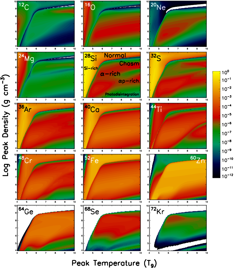
Figure 2: Final mass fractions of the $\alpha$-chain isotopes ($\mathrm{{}^{56}Ni}$ omitted) in the peak temperature–density plane for the exponential profile at $Y_{e}=0.5$. The white colored space corresponds to values below the color scale shown. From left to right, the first row corresponds to $\mathrm{{}^{12}C}$, $\mathrm{{}^{16}O}$ and $\mathrm{{}^{20}Ne}$, the second row corresponds to $\mathrm{{}^{24}Mg}$, $\mathrm{{}^{28}Si}$ and $\mathrm{{}^{32}S}$, the third row corresponds to $\mathrm{{}^{36}Ar}$, $\mathrm{{}^{40}Ca}$ and $\mathrm{{}^{44}Ti}$, the fourth row corresponds to $\mathrm{{}^{48}Cr}$, $\mathrm{{}^{52}Fe}$ and $\mathrm{{}^{60}Zn}$, and the fifth row corresponds to $\mathrm{{}^{64}Ge}$, $\mathrm{{}^{68}Se}$ and $\mathrm{{}^{72}Kr}$.

Figure 2 shows the final mass fractions of isotopes along the $\alpha$-chain for initially symmetric matter ($Y_{e}=0.5$). The temperature–density planes include the full range of peak conditions within our parameter space. With the exception of $\mathrm{{}^{56}Ni}$ (not shown), the topological structure of all planes is similar, and is marked by distinct regions. These regions are labeled in the $\mathrm{{}^{28}Si}$ contour plot for the symmetric case, each region corresponding to a type of freeze-out expansion. Further types of freeze-out expansions are manifested for initial electron fraction $Y_{e}\neq 0.5$ (see analysis below). The aggregate range of isotopes produced by all identified freeze-out types is in the mass range $12\leqslant A\leqslant 122$, including in addition the free neutrons, protons, and $\alpha$-particles. The structure of the temperature–density plane is very similar among the majority of the isotopes in this mass range. We classify into a family the isotopes within the mass range $12\leqslant A\leqslant 122$ whose temperature–density plane features a region-divided structure (henceforth the “first family” of isotopes) and explore the common features that these isotopes share. The $\alpha$-chain isotopes shown in Figure 2 belong to the first family.

The mass fraction profiles per region for the isotopes in Figure 2 and the first family overall are similar, indicating that within a region the isotopes of this family are produced by the same mechanism. The mass fraction profile similarities arise from the initial formation of a large-scale QSE cluster during the freeze-out processes. Within the cluster all nuclei are interconnected with reactions in equilibrium, and mass fraction values are determined by the temperature, density and electron fraction variations based on minimization principles of the Helmholtz free energy (Seitenzahl et al., 2008). Subsequent ESTs alter the shape of the QSE cluster and eventually the cluster dissolves. The precise locus of the regions in the temperature–density plane for an isotope of the first family depends on the local equilibrium patterns near the isotope while the large QSE cluster dissolves.

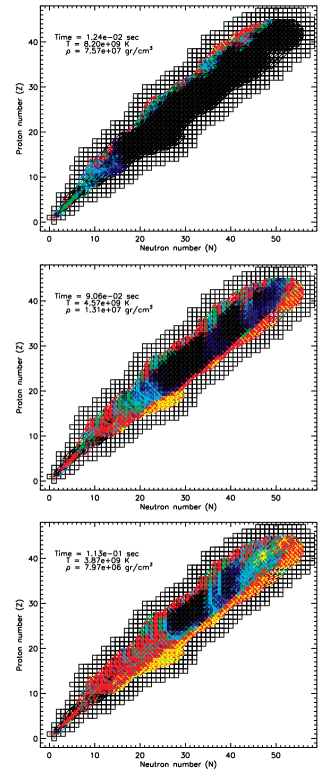
Figure 3: QSE cluster motion in the chart of nuclides for an $\alpha$-rich freeze-out. The QSE cluster remnant condenses near the magic number 28. Each colored line corresponds to a nuclear reaction and indicates the level of nuclear flow transferred between the isotopes connected. Normalized flows $\phi$ are colored black for $0\leq\phi<0.01$, navy for $0.01\leq\phi<0.05$, blue for $0.05\leq\phi<0.1$, cyan for $0.1\leq\phi<0.4$, green for $0.4\leq\phi<0.8$, red for $0.8\leq\phi<1.0$, and yellow for $\phi$=1.0. Small $\phi$ values indicate reactions in equilibrium, while $\phi$=1.0 implies pure one-way nuclear flow transfer.

Figure 3 illustrates the upward shifting in mass of the QSE cluster (Meyer et al., 1998). The QSE cluster remnant condenses around the magic number 28, and nuclei in this small group tend to dominate the final composition. The isotopes of the first family which are gradually left outside the QSE cluster form chains of $\mathrm{(p,\gamma)}$ reactions in equilibrium along the isotone lines. The first EST related to these isotopes’ exit from the QSE cluster is signaled at the microscopic level by the equilibrium break of the $\alpha$-capture reactions linking the $\mathrm{(p,\gamma)}$ equilibrium chains. During the $\alpha$$p$-rich freeze-out, isotopes of the first family sustain a second EST when certain $\mathrm{(p,\gamma)}$ reactions in the isotone chain break equilibrium. These small-scale equilibrium patterns are responsible for producing eventually the isotopes of the first family from $\mathrm{{}^{12}C}$ to the iron peak. On the contrary, the formation of the chasm for each isotope of the first family results from the dissolution of the large-scale QSE cluster to two smaller ones. The first cluster encompasses the silicon group elements and the second cluster encompasses the iron group elements. The cluster breakage results in massive flow transfer from the silicon and most of the iron group isotopes toward a small group of nuclides near the magic number 28. The flow transfer proceeds until all mass fractions are depleted, excluding the mass fractions of nuclei around the magic number 28. These nuclei are produced in large amounts and dominate the final composition.

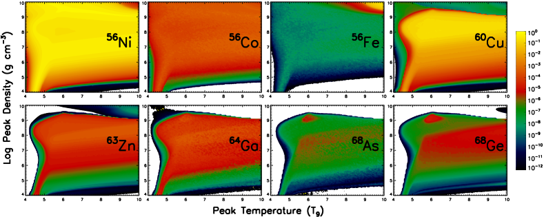
Figure 4: Final mass fractions of isotopes with protons and neutrons near the magic number 28 (second family) in the peak temperature–density plane for the power-law profile at $Y_{e}=0.52$. The white colored space corresponds to values below the color scale shown. From left to right, the first row corresponds to $\mathrm{{}^{56}Ni}$, $\mathrm{{}^{56}Co}$, $\mathrm{{}^{56}Fe}$ and $\mathrm{{}^{60}Cu}$, and the second row corresponds to $\mathrm{{}^{63}Zn}$, $\mathrm{{}^{64}Ga}$, $\mathrm{{}^{68}As}$ and $\mathrm{{}^{68}Ge}$.

The types of freeze-out discussed so far (normal, $\alpha$-rich, $\alpha$$p$-rich, and the chasm) tend to favor the production of nuclei with proton and neutron numbers in the locality of the magic number 28. Figure 4 shows a sample of such nuclei, and Table 2 provides the complete list. These isotopes tend to dominate the final composition for most initial electron fraction values. The final mass fractions in Figure 4 demonstrate homogeneous structures within the temperature–density plane, implying that these isotopes do not sustain any EST during the evolution. The restriction of the remnant QSE cluster and the accumulation of nuclear flow among these isotopes are responsible for the absence of ESTs. The accumulation of flow stems from the fact that nuclei with proton or neutron numbers near the magic number 28 tend to maximize their binding energy per nucleon. As a result, such nuclei are relatively more bound compared to nuclei with nucleon numbers far from the magic number values, and their production within a network of reactions is favored. We classify isotopes which do not sustain any EST during freeze-out expansions and tend to dominate the final composition into a “second family” of isotopes. We have demonstrated that nuclei whose neutron or proton number is near the magic number 28 belong to the second family. Below, we show that nuclei with neutron numbers near the magic numbers 50 and 82 also belong to the second family.

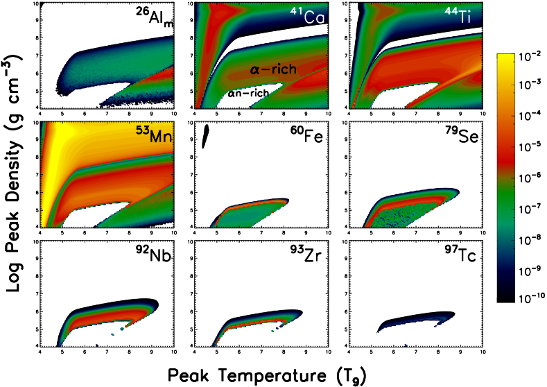
Figure 5: Final mass fractions of select radioactivities in the peak temperature -density plane for the exponential profile at $Y_{e}=0.48$. The white colored space corresponds to values below the color scale shown. From left to right, the first row corresponds to $\mathrm{{}^{26}Al}$_m, $\mathrm{{}^{41}Ca}$, and $\mathrm{{}^{44}Ti}$, the second row corresponds to $\mathrm{{}^{53}Mn}$, $\mathrm{{}^{60}Fe}$, and $\mathrm{{}^{79}Se}$, and the third row corresponds to $\mathrm{{}^{92}Nb}$, $\mathrm{{}^{93}Zr}$, and $\mathrm{{}^{97}Tc}$. The $\alpha$-rich and $\alpha$$n$-rich freeze-out regions are labeled on the temperature–density plane for $\mathrm{{}^{41}Ca}$.

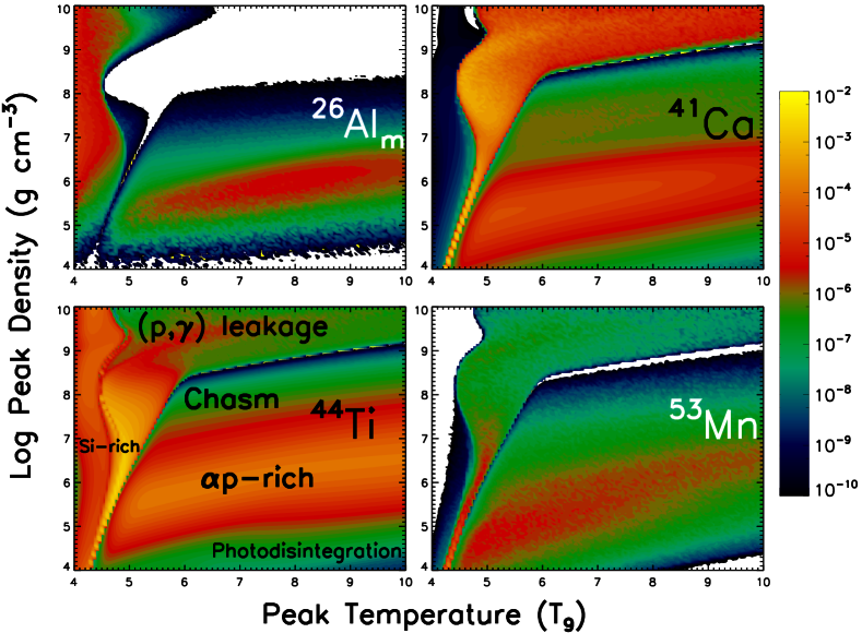
Figure 6: Final mass fractions of select radioactivities in the peak temperature -density plane for the exponential profile at $Y_{e}=0.52$. The white colored space corresponds to values below the color scale shown. From left to right, the first row corresponds to $\mathrm{{}^{26}Al}$_m, and $\mathrm{{}^{41}Ca}$, and the second row corresponds to $\mathrm{{}^{44}Ti}$ and $\mathrm{{}^{53}Mn}$.

Figures 5 and 6 show the temperature–density planes of select radioactivities up to mass $A=97$ which have non-negligible yields for the corresponding initial $Y_{e}$ values. The regions of the $\alpha$$n$-rich freeze-out and $\mathrm{(p,\gamma)}$-leakage regime are labeled. These two types of freeze-out expansions are not manifested for initially symmetric matter. The temperature–density planes depict a region-divided structure, indicating that these radioactivities belong to the first family of isotopes. The decay timescale of $\mathrm{{}^{26}Al}$_m is approximately 2 s. Consequently, yield values are seen only for the exponential profile where the expansion timescale is less than a second, while for the power-law it decays prior to complete freeze-out. On the contrary, $\mathrm{{}^{26}Al}$_g is mostly produced during the power-law expansion for $Y_{e}\geqslant 0.5$. $\mathrm{{}^{41}Ca}$ is produced during the $\alpha$-rich and $\alpha$$p$-rich freeze-outs for the full range of our initial electron fraction values, and also during the $\mathrm{(p,\gamma)}$-leakage regime (Figure 6) for the exponential profile and $Y_{e}>0.5$. The $\mathrm{(\alpha,\gamma)}$ and $\mathrm{(\alpha,p)}$ channels control its production for $Y_{e}=0.48$, while the $\mathrm{(p,\gamma)}$ and the weak reactions impact its synthesis for $Y_{e}\geqslant 0.5$. In addition, the $\mathrm{(\alpha,p)}$ channels shape the locus of the borderline between the $\mathrm{(p,\gamma)}$-leakage and Si-rich regimes in the contour plot for $Y_{e}>0.5$. $\mathrm{{}^{53}Mn}$ is produced mostly during the normal freeze-out for $Y_{e}\leqslant 0.5$, although it has significant yields from the $\alpha$-rich and $\alpha$$p$-rich freeze-outs for the power-law expansion. It is relatively insensitive to reaction rates for $Y_{e}<0.5$, while the $\mathrm{(p,\gamma)}$ and weak reactions have significant impact for $Y_{e}\geqslant 0.5$. The $\mathrm{(\alpha,p)}$ and $\mathrm{(p,\gamma)}$ channels affect the borderline between the $\mathrm{(p,\gamma)}$-leakage and Si-rich regimes.

Radioactivities heavier than mass $A=60$ are produced primarily in neutron-rich environments for the exponential and power-law profiles. Specifically, they may either be produced during an $\alpha$$n$-rich freeze-out (Woosley & Hoffman, 1992) or by a process that combines features between the $\alpha$-rich and $\alpha$$n$-rich freeze-outs (Figure 5). The $\alpha$$n$-rich freeze-out occurs for relatively low initial electron fraction values and its locus is constrained to regions of low peak densities in the contour plots. The combination of high peak temperatures and low peak densities allows the establishment of a photodisintegration regime early in the evolution. The balance between the $\mathrm{p(e^{-},\nu_{e})n}$ and $\mathrm{n(e^{+},\overline{\nu_{e}})p}$ reactions maintains the electron fraction values below 0.5, which favor an overproduction of neutrons against protons. Such values for $Y_{e}$ allow the major nuclear flows to bypass the doubly magic nucleus $\mathrm{{}^{56}Ni}$ and heavier elements are produced (Hartmann et al., 1985; Woosley & Hoffman, 1992; Magkotsios et al., 2010). The QSE cluster shifts upward in mass, but it is not localized solely around the magic number 28. Instead, neutron capture reactions shift the cluster to heavier masses and pile up nuclear flow in the locality of nuclei with neutron magic numbers 50 and 82. The concentration of nuclear flow around these nuclei maintains the equilibrium structure in their locality and prevents them from sustaining ESTs. Once again, the flow concentration near nuclei with magic numbers 50 and 82 is a nuclear structure effect. These nuclei maximize locally the nuclear binding energy per nucleon and are relatively more bound compared to other nuclei with nucleon numbers away from the magic number series. Consequently, isotopes such as $\mathrm{{}^{86}Kr}$, $\mathrm{{}^{87}Rb}$, $\mathrm{{}^{88}Sr}$, and $\mathrm{{}^{122}Zr}$ belong to the second family of isotopes and dominate the final composition along with free $\alpha$-particles and neutrons. During the evolution, the excess of free neutrons guarantees a large-scale equilibrium structure maintained primarily by chains of $\mathrm{(n,\gamma)}$ and $\mathrm{(p,n)}$ reactions in equilibrium. Isotopes of the first family with mass $A\gtrsim 60$ including the radioactivities $\mathrm{{}^{60}Fe}$ and $\mathrm{{}^{79}Se}$ sustain an EST when $\mathrm{(p,n)}$ reactions in their locality break equilibrium.

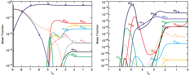
Figure 7: Mass fraction evolution of dominant yields (left panel) and radioactivities (right panel) for the transition region between the $\alpha$-rich and $\alpha$$n$-rich freeze-outs. Initial conditions are $T_{9}=9$, $\rho=5\times 10^{7}$ g cm^-3, and $Y_{e}=0.48$ for the power-law profile (3304 isotope network).

The production of radioactivities such as $\mathrm{{}^{92}Nb}$, $\mathrm{{}^{93}Zr}$, and $\mathrm{{}^{97}Tc}$ by the exponential and power-law expansions is favored only within the narrow transition region between the $\alpha$-rich and $\alpha$$n$-rich freeze-outs. Figure 7 shows the mass fraction evolution of dominant elements and radioactivities within this region. The free neutrons are depleted below the NSE threshold and do not allow the neutron capture reactions to shift the QSE cluster until the magic number 82. The flows are blocked around the magic number 50. This effect is illustrated in Figure 8. The yields of $\mathrm{{}^{86}Kr}$, $\mathrm{{}^{87}Rb}$, and $\mathrm{{}^{88}Sr}$ still dominate the final composition, but are slightly enhanced compared to the region of the $\alpha$$n$-rich freeze-out. The constraint of nuclear flow near $\mathrm{{}^{86}Kr}$ maximizes the yields of $\mathrm{{}^{60}Fe}$ and $\mathrm{{}^{79}Se}$, and allows the production of $\mathrm{{}^{92}Nb}$, $\mathrm{{}^{93}Zr}$, and $\mathrm{{}^{97}Tc}$ (Figure 5).

5 REACTION RATE SENSITIVITY STUDY FOR SELECT RADIOACTIVITIES

We perform a sensitivity study on reaction rates related to the synthesis of radioactivities for the exponential and power-law expansions, to identify the reactions which are primarily responsible for their production in core-collapse supernovae. These critical reactions determine whether an EST takes place or not. Reaction channels and individual rates are either multiplied by a factor or removed from the network. Strong reaction rates are multiplied by factors of 100 or 0.01, while the corresponding factors for the weak reactions are 1000 or 0.001. These factors are adequate to facilitate the identification of trends in the yields, although they exceed experimental uncertainties in most cases. Sensitivity studies where reactions were varied within experimental uncertainty ranges have been performed by Hoffman et al. (2010) and Tur et al. (2010). Our calculations include rates for weak interactions (Fuller et al., 1980, 1982b, 1982a; Oda et al., 1994; Langanke & Martínez-Pinedo, 2001), the theoretical rates of Rauscher & Thielemann (2000), and select experimental rates for capture and photodisintegration reactions.

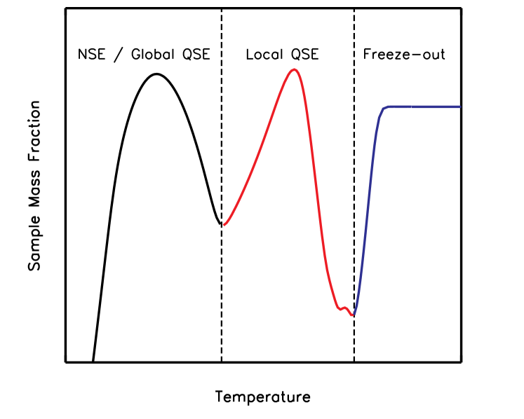
Figure 9: Mass fraction schematic for decreasing temperature, where the arc structure is illustrated. Such mass fraction profiles are representative of the chasm, $\alpha$-rich, $\alpha$$p$-rich, and $\alpha$$n$-rich freeze-outs. The first arc (black) describes the mass fraction trend during a large-scale QSE state. The second arc (red) describes the mass fraction trend once the isotope is outside the large equilibrium cluster, and its trends may be explained by local equilibrium states (local QSE). The blue ascending track is denoted as third arc, and is related to a mixture of local QSE and non-equilibrium nucleosynthesis. Mass fractions during an $\alpha$-rich freeze-out have only an ascending track past the first arc, while for the chasm region the mass fractions have only one arc.

The structure of the temperature–density plane for isotopes of the first family is affected by certain key reactions per isotope, in combination with the expansion timescale. Specific reactions such as the 3$\alpha$, $\alpha\alpha n$, $\mathrm{p(e^{-},\nu_{e})n}$, $\mathrm{n(e^{+},\overline{\nu_{e}})p}$, and combinations of a large number of weak reactions impact all mass fractions simultaneously either by transferring nuclear flow to the QSE cluster, or by contributing to electron fraction variations (Fuller & Meyer, 1995; McLaughlin & Fuller, 1995; McLaughlin et al., 1996; Aprahamian et al., 2005; Surman & McLaughlin, 2005; Liebendörfer et al., 2008). However, the local equilibrium patterns are controlled by reactions in the locality of each isotope. Table 3 lists the reactions that impact the synthesis of radioactivities in the mass range $12\leqslant A\leqslant 122$ produced during freeze-out expansions. In Table 3 the contribution of a reaction is focused on specific parts of the isotope’s mass fraction curve. Below we use the term “arc” frequently, so it is convenient to provide a visualization of this structure. Figure 9 shows a sample mass fraction evolution of an isotope for decreasing temperature. Two local minimum points of the mass fraction curve are identified. These points separate the curve in three parts (arcs). The first part (black arc) is related to the mass fraction evolution when the isotope participates in a large-scale QSE cluster (global QSE). The second and third parts (red and blue arcs respectively) are related to mass fraction trends when the isotope either participates in small-scale equilibrium clusters (local QSE) or does not belong to any cluster at all (non-equilibrium nucleosynthesis). Since the third arc is not a full arc, it is also mentioned as “ascending track”. Note that the mass fraction curve may be limited to two arcs, i.e. the first arc and the ascending track until freeze-out (for instance, see Figure 7).

The $\mathrm{{}^{26}Al}$ yield has an average value $X(\mathrm{{}^{26}Al})\sim 10^{-7}$ within the $\alpha$-rich and $\alpha$$p$-rich freeze-out regimes for the exponential profile only, where the metastable state $\mathrm{{}^{26}Al}$_m has significant yield (Figures 5 and 6). $\mathrm{\mathrm{{}^{26}Al}_{g}(p,\gamma)\mathrm{{}^{27}Si}}$ and $\mathrm{\mathrm{{}^{26}Al}_{g}(\alpha,p)\mathrm{{}^{29}Si}}$ configure the chasm features and the characteristic arcs in the mass fraction profiles during the $\alpha$-rich and $\alpha$$p$-rich freeze-outs. They also control the flow between the $N=13$ and $N=15$ isotones. The equilibrium break of $\mathrm{\mathrm{{}^{26}Al}_{g}(\alpha,p)\mathrm{{}^{29}Si}}$ marks the appearance and controls the depth of the chasm in the contour plot and the first dip in the $\mathrm{{}^{26}Al}$ mass fraction profile. The equilibrium break of $\mathrm{\mathrm{{}^{26}Al}_{g}(p,\gamma)\mathrm{{}^{27}Si}}$ during the $\alpha$$p$-rich freeze-out transfers flow from $\mathrm{{}^{26}Al}$ to heavier isotopes along the $N=13$ isotone and configures the shape and dip of the second arc in the $\mathrm{{}^{26}Al}$ mass fraction. Additional reactions that contribute similarly are $\mathrm{\mathrm{{}^{25}Mg}(p,\gamma)\mathrm{{}^{26}Al}_{g}}$, $\mathrm{\mathrm{{}^{25}Al}(p,\gamma)\mathrm{{}^{26}Si}}$, $\mathrm{\mathrm{{}^{26}Si}(p,\gamma)\mathrm{{}^{27}P}}$, and $\mathrm{\mathrm{{}^{27}P}(p,\gamma)\mathrm{{}^{28}S}}$. The $\mathrm{\mathrm{{}^{24}Mg}(\alpha,\gamma)\mathrm{{}^{28}Si}}$ reaction distributes flow within the silicon group and shapes the ascending track to the $\mathrm{{}^{26}Al}$ mass fraction past the arcs during the $\alpha$$p$-rich freeze-out. The yield of $\mathrm{{}^{26}Al}$ is largely dependent on the collective flow transfer by weak reactions toward symmetric nuclei. Specific weak reactions with the largest contribution for $\mathrm{{}^{26}Al}$ are listed in Table 3.

$\mathrm{{}^{41}Ca}$ is an example of composite contribution from $\mathrm{(p,\gamma)}$ reactions along its own and neighboring isotone lines which are connected by $\mathrm{(\alpha,\gamma)}$ reactions. Table 3 lists the related reactions for $Y_{e}\geqslant 0.5$, and reactions that transfer flow for neutron-rich compositions. For proton-rich environments $\mathrm{{}^{41}Ca}$ is also dependent on the collective flow transfer by weak reactions.

Radioactivities with mass $A\gtrsim 60$ depend mostly on neutron captures and weak reactions. The yield of $\mathrm{{}^{53}Mn}$ depends only on the collective flow transfer by weak reactions. The weak reactions with the largest contribution are listed in Table 3. $\mathrm{\mathrm{{}^{86}Kr}(\alpha,n)\mathrm{{}^{89}Sr}}$ is the main flow distributor within the small cluster in the locality of the neutron magic number $N=50$ and it affects the mass fractions of $\mathrm{{}^{60}Fe}$, $\mathrm{{}^{79}Se}$, $\mathrm{{}^{92}Nb}$, $\mathrm{{}^{93}Zr}$, and $\mathrm{{}^{97}Tc}$. $\mathrm{\mathrm{{}^{60}Fe}(p,n)\mathrm{{}^{60}Co}}$ shapes the second arc of the $\mathrm{{}^{60}Fe}$ mass fraction, and its strength determines the degree of the yield’s depletion. $\mathrm{\mathrm{{}^{60}Fe}(\alpha,n)\mathrm{{}^{63}Ni}}$ contributes to the formation of the arc, while $\mathrm{\mathrm{{}^{59}Fe}(n,\gamma)\mathrm{{}^{60}Fe}}$ and $\mathrm{\mathrm{{}^{58}Fe}(\alpha,n)\mathrm{{}^{61}Ni}}$ regulate the arc’s amplitude and slope respectively. Most notably, $\mathrm{\mathrm{{}^{60}Fe}(n,\gamma)\mathrm{{}^{61}Fe}}$ does not impact the $\mathrm{{}^{60}Fe}$ mass fraction and yield for the freeze-out expansions. The mass fraction profile of $\mathrm{{}^{79}Se}$ is marked by a sharp ascending track at complete freeze-out which increases the yield by an order of magnitude. The abrupt flow transfer stems mostly from the collective contribution of the weak reactions, with major contribution from $\mathrm{\mathrm{{}^{79}As}(,e^{-}\;\nu_{e})\mathrm{{}^{79}Se}}$. Additional reactions that contribute to this ascending track prior to freeze-out are $\mathrm{\mathrm{{}^{77}Se}(n,\gamma)\mathrm{{}^{78}Se}}$ and $\mathrm{\mathrm{{}^{78}Se}(n,\gamma)\mathrm{{}^{79}Se}}$. Its mass fraction arc is formed by $\mathrm{\mathrm{{}^{79}As}(p,n)\mathrm{{}^{79}Se}}$. Similarly, the mass fraction arc for $\mathrm{{}^{92}Nb}$ is formed by $\mathrm{\mathrm{{}^{92}Zr}(p,n)\mathrm{{}^{92}Nb}}$, and the arc for $\mathrm{{}^{97}Tc}$ by $\mathrm{\mathrm{{}^{97}Mo}(p,n)\mathrm{{}^{97}Tc}}$, $\mathrm{\mathrm{{}^{97}Tc}(n,\gamma)\mathrm{{}^{98}Tc}}$, and $\mathrm{\mathrm{{}^{98}Mo}(p,n)\mathrm{{}^{98}Tc}}$. $\mathrm{{}^{93}Zr}$ is in the locality of the neutron magic number $N=50$, and its mass fraction profile monotonically increases up to $X(\mathrm{{}^{93}Zr})\sim 10^{-4}$ in the transition region between the $\alpha$-rich and $\alpha$$n$-rich freeze-outs. The rate strength of $\mathrm{\mathrm{{}^{92}Zr}(n,\gamma)\mathrm{{}^{93}Zr}}$ shapes the yield value by transferring flow to $\mathrm{{}^{93}Zr}$ from the isotopes with neutron number $N=50$.

6 YIELDS FROM NON-MONOTONIC PROFILES

The exponential and power-law profiles discussed so far involve the initial formation of a large-scale QSE cluster and subsequent states of small-scale clusters. Non-equilibrium nucleosynthesis appears only during the freeze-out stage at the end of the evolution. The non-monotonic expansion profiles (Section 3) may have non-equilibrium intervals followed by the formation of a large-scale QSE cluster, resulting in final compositions which cannot be achieved by monotonic profiles. Table 4 lists the differences between the monotonic and non-monotonic profiles. The keywords related to the evolution of the QSE cluster are “hierarchical” and “periodic” for the monotonic and non-monotonic profiles respectively. The term hierarchical denotes the gradual dissolution of the single large-scale QSE cluster to multiple small-scale clusters, while the term periodic describes the sequence of transitions from NSE and global QSE, to local QSE and non-equilibrium phase, to global QSE again and then local QSE and non-equilibrium phase until freeze-out.

The existence of ESTs during non-monotonic profiles depends on the combination of the extremum point values for the temperature and density. Arcones et al. (2007) report ranges of $0.4\leqslant T_{9}\leqslant 2$ and $10^{2}\leqslant\rho\leqslant 10^{4}$ g cm^-3 for the temperature and density behind the reverse shock, while Wanajo et al. (2011) report a temperature range of $1.5\leqslant T_{9}\leqslant 3$. The flow transfer by reactions out of equilibrium among scattered small-scale equilibrium clusters impacts the mass fraction evolution dramatically. The flow patterns are very sensitive to variations in the values of the temperature and density extremum points. This sensitivity diversifies the production mechanisms significantly. Table 5 lists the combinations of temperature and density extremum points within our data set which tend to maximize the yields of radioactivities. The peak temperature for the non-monotonic expansions is chosen to be $T_{9}=9$, and the peak density and initial electron fraction values range between $10^{6}\leqslant\rho\leqslant 10^{8}$ g cm^-3 and $0.48\leqslant Y_{e}\leqslant 0.52$ respectively. These peak temperature and density values are large enough to establish NSE early in the evolution, so that the initial composition dependence is removed. Below we present the details of certain profiles which produce simultaneously most of the radioactivities in the mass range $12\leqslant A\leqslant 122$. These radioactive isotopes could be transferred to upper (cooler) mass layers by mixing processes during the explosion, where the effective lifetime of the radioactivities is longer (Tur et al., 2010), and possibly released to the interstellar medium.

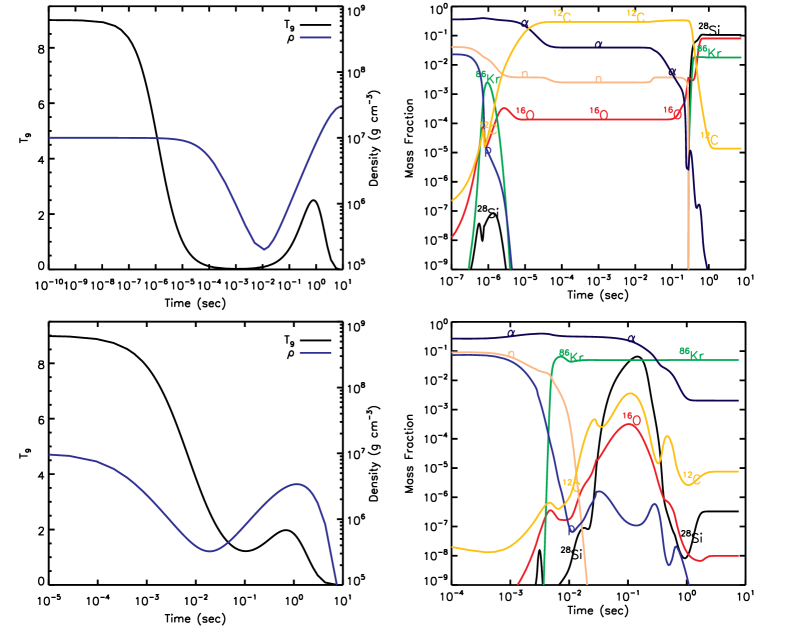
Figure 10: Non-monotonic temperature and density trajectories (left column) and key mass fraction profiles (right column) for initial conditions $T_{9}=9$, $\rho=10^{7}$ g cm^-3, and $Y_{e}=0.48$. The top row is a profile where the $\mathrm{{}^{60}Fe}$ yield is approximately maximized, while the profile at the bottom row tends to maximize the $\mathrm{{}^{44}Ti}$ yield within our data set.

Figure 10 shows the thermodynamic and mass fraction evolutions of two non-monotonic profiles for initially neutron-rich composition ($Y_{e}=0.48$). The extremum values for the profile of the top row are $T_{9}^{min}=0.02$, $T_{9}^{max}=2.5$, $\rho_{min}=2\times 10^{5}$ g cm^-3, and $\rho_{max}=3\times 10^{7}$ g cm^-3. This profile approximately maximizes the $\mathrm{{}^{60}Fe}$ yield within our data set. During the initial temperature decrement (until $t=10^{-4}$ s) the density is relatively fixed to its peak value. The conditions at the $T_{9}=5$ NSE threshold are similar to an $\alpha$-rich freeze-out in neutron-rich matter, where the 3$\alpha$ forward rate dominates its inverse photodisintegration and the protons are rapidly consumed. However, the temperature evolution is fast enough that it prevents significant flow transfer beyond $\mathrm{{}^{16}O}$, and the QSE cluster dissolves without shifting upward in mass. The temperature nearly reaches freeze-out levels after $t=10^{-4}$ s, and $\mathrm{{}^{12}C}$ dominates the composition, with significant mass fraction values for free neutrons, $\alpha$-particles, and $\mathrm{{}^{16}O}$. The density decrease from $t=10^{-4}$ s until $t=10^{-2}$ s does not impact the mass fractions due to low temperature values. The subsequent temperature and density increase result in carbon burning primarily by the $\mathrm{\mathrm{{}^{12}C}(\mathrm{{}^{12}C},p)\mathrm{{}^{23}Na}}$ and $\mathrm{\mathrm{{}^{12}C}(\mathrm{{}^{12}C},\alpha)\mathrm{{}^{20}Ne}}$ reactions. A second large-scale QSE cluster is formed and the low electron fraction values in combination with the free neutron abundance guarantee flow transfer near $\mathrm{{}^{86}Kr}$ through $\mathrm{(n,\gamma)}$ and $\mathrm{(p,n)}$ reactions. The temperature maximum is slightly lower than the typical silicon burning threshold $T_{9}\sim 3$ (Iliadis, 2007) at $t=1$ s, and the final composition is dominated mostly by carbon burning products and elements in the locality of the $N=50$ neutron magic number, while elements near the $N=28$ magic number are severely underproduced. The final composition includes significant yields for the radioactivities listed in Table 5, excluding $\mathrm{{}^{44}Ti}$ and $\mathrm{{}^{97}Tc}$.

The second row of Figure 10 corresponds to a profile with extremum values $T_{9}^{min}=1.4$, $T_{9}^{max}=1.94$, $\rho_{min}=3.3\times 10^{5}$ g cm^-3, and $\rho_{max}=3.4\times 10^{6}$ g cm^-3. This profile approximately maximizes the $\mathrm{{}^{44}Ti}$ yield within our data set. The flow transfer by the 3$\alpha$ rate to the QSE cluster occurs over a longer interval compared to the profile of the top row in Figure 10. The QSE cluster shifts upward in mass until the $N=50$ neutron magic number, producing $\mathrm{{}^{86}Kr}$ and the radioactivities $\mathrm{{}^{92}Nb}$, $\mathrm{{}^{93}Zr}$ and $\mathrm{{}^{97}Tc}$. Up to the point where the $\mathrm{{}^{86}Kr}$ abundance is maximized (near $t=10^{-2}$ s), the process resembles the evolution of exponential and power-law profiles in the transition regime between the $\alpha$-rich and $\alpha$$n$-rich freeze-outs (see Section 4 and Figure 7). The first $\alpha$-capture reactions to break equilibrium appear in the mass region of $\mathrm{{}^{12}C}$ and $\mathrm{{}^{16}O}$. The increasing number of $\alpha$-capture reactions which break equilibrium within this mass region and the silicon group shift the low mass border of the QSE cluster toward heavier nuclei. The $\alpha$-capture reactions with the largest net flows are blocked within the silicon group, because the Coulomb repulsion for the specific thermodynamic conditions prevents the $\alpha$-capture reactions involving heavier nuclei from acquiring large flow values. However, the QSE cluster continues to shift upward in mass. The blockage of the largest flows for the $\alpha$-captures is a non-equilibrium effect, and the precise nuclear mass range where these large flows are localized in depends on the details of the specific expansion profile. For the profile of the bottom row in Figure 10 the largest flows shift in mass until the $\mathrm{{}^{40}Ca}$ – $\mathrm{{}^{44}Ti}$ – $\mathrm{{}^{48}Cr}$ region and produce these isotopes with a mass fraction $X\sim 10^{-3}$. The largest flows shift downward in mass next, while the temperature approaches its minimum value at time $t=10^{-1}$ s. At this time, the $\mathrm{{}^{28}Si}$ mass fraction reaches its maximum value (bottom right panel in Figure 10). The subsequent temperature and density increase until time $t=1$ s relocates the largest flows for the $\alpha$-captures back to the $\mathrm{{}^{40}Ca}$ – $\mathrm{{}^{44}Ti}$ – $\mathrm{{}^{48}Cr}$ region at the cost of the $\mathrm{{}^{28}Si}$ abundance. $\mathrm{{}^{44}Ti}$ dominates the final composition with a yield $X(\mathrm{{}^{44}Ti})=0.286$. Other isotopes to be produced in significant amounts include $\mathrm{{}^{41}Ca}$ and $\mathrm{{}^{53}Mn}$. Isotopes near the mass $A=56$ are underproduced, since their equilibrium abundances are not favored by the QSE formation, and the largest flows of $\alpha$-capture reactions never reach this mass region.

The non-monotonic profiles of Figure 10 demonstrate cases of final compositions which cannot be achieved by monotonic profiles, such as the exponential and power law profiles. Both non-monotonic expansions include significant intervals of non-equilibrium nucleosynthesis followed by the reformation of equilibrium clusters. This feature results in a final composition dominated by silicon group elements which belong to the first family of isotopes, and neutron-rich isotopes of the second family near the mass $A=86$. Isotopes of the second family near the mass $A=56$ are underproduced. During monotonic expansions, the QSE cluster size decreases gradually during the evolution and the non-equilibrium part of nucleosynthesis is always constrained near freeze-out. This feature results in the dominance of isotopes in the second family only, and does not allow patterns such as those of Figure 10.

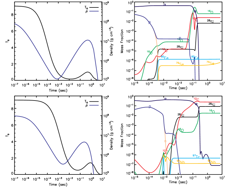
Figure 11: Non-monotonic temperature and density trajectories (left column) and key mass fraction profiles (right column) for initial conditions $T_{9}=9$, $\rho=10^{8}$ g cm^-3, and $Y_{e}=0.50$. The top row is a profile where the $\mathrm{{}^{60}Fe}$ yield is approximately maximized, while the profile at the bottom row tends to maximize the $\mathrm{{}^{97}Tc}$ yield within our data set.

The mixing processes during the supernova explosion impact significantly the nucleosynthesis mechanisms. The majority of one-dimensional supernova models tend to position the mass-cut near the region where the electron fraction begins to decrease below $Y_{e}=0.5$ (Woosley et al., 1973; Weaver & Woosley, 1993; Woosley & Weaver, 1995; Thielemann et al., 1996; Rauscher et al., 2002; Woosley et al., 2002; Limongi & Chieffi, 2003; Chieffi & Limongi, 2004). As a result, the subsequent supernova shock wave in these models traverses material which has initially symmetric or nearly symmetric composition. Our exponential and power-law analysis has demonstrated that the radioactivities for $A\geqslant 60$ are not produced in significant amounts during explosions within symmetric matter which lack mixing processes. However, there exist types of non-monotonic profiles which produce these isotopes even for initially symmetric matter. Figure 11 shows two such profiles.

The profile in the top row of Figure 11 has extremum values $T_{9}^{min}=0.157$, $T_{9}^{max}=1.01$, $\rho_{min}=1.177\times 10^{5}$ g cm^-3, and $\rho_{max}=1.13\times 10^{7}$ g cm^-3, and maximizes the $\mathrm{{}^{60}Fe}$ yield within our data set. During the non-equilibrium part of the evolution the QSE cluster dissolves in multiple small-scale clusters. The dominant yields are determined by $\alpha$-capture reactions within the mass range $12\lesssim A\lesssim 48$, which is a non-equilibrium and profile dependent effect. Yields for masses $A\gtrsim 60$ are configured by the interplay of (1) $\mathrm{(n,\gamma)}$ reactions out of equilibrium which supply the nuclear flow to $A\gtrsim 60$ nuclei at the cost of free neutrons, (2) $\mathrm{(p,n)}$ reactions out of equilibrium which redistribute the nuclear flow among neutron-rich isotopes, and (3) the small-scale chains of $\mathrm{(p,n)}$ reactions in equilibrium along isobars which collect the majority of nuclear flow available. For instance, equilibrium chains along isobars near $\mathrm{{}^{60}Fe}$ include $\mathrm{{}^{58}Cu}$ to $\mathrm{{}^{58}Fe}$ for mass $A=58$, $\mathrm{{}^{59}Cu}$ to $\mathrm{{}^{59}Co}$ for mass $A=59$, $\mathrm{{}^{60}Zn}$ to $\mathrm{{}^{60}Ni}$ for mass $A=60$, $\mathrm{{}^{61}Zn}$ to $\mathrm{{}^{61}Ni}$ for mass $A=61$, and $\mathrm{{}^{62}Zn}$ to $\mathrm{{}^{62}Ni}$ for mass $A=62$. Although $\mathrm{{}^{60}Fe}$ does not participate in the $A=60$ equilibrium chain, it controls the amount of incoming flow from the $Z=26$ isotopic line that is transferred to the $A=60$ chain through the reactions $\mathrm{\mathrm{{}^{60}Fe}(p,n)\mathrm{{}^{60}Co}}$ and $\mathrm{\mathrm{{}^{60}Co}(p,n)\mathrm{{}^{60}Ni}}$. Once the free neutrons are depleted, the mass fractions in this mass range are stabilized until freeze-out. The top right panel of Figure 11 shows that $\mathrm{{}^{79}Se}$ is also produced. Its mass fraction increase close to freeze-out stems from the action of weak reactions (see Section 5).

The interplay between $\mathrm{(n,\gamma)}$ and $\mathrm{(p,n)}$ reactions for initial $Y_{e}=0.5$ is another example of non-equilibrium nucleosynthesis. The formation of small-scale equilibrium patterns is strongly dependent on the particular combinations of temperature and density values during the expansion. The profile in the bottom row of Figure 11 looks similar to the profile in the top row. It has extremum values $T_{9}^{min}=0.55$, $T_{9}^{max}=1.41$, $\rho_{min}=3.4\times 10^{5}$ g cm^-3, and $\rho_{max}=4.5\times 10^{6}$ g cm^-3. The mass fraction curves in the right column of the Figure have similar trends, but the yields’ distribution is different. $\mathrm{{}^{16}O}$ is underproduced with respect to $\mathrm{{}^{12}C}$ and $\mathrm{{}^{28}Si}$, and the production of $\mathrm{{}^{97}Tc}$ and $\mathrm{{}^{92}Nb}$ is favored instead of $\mathrm{{}^{60}Fe}$ and $\mathrm{{}^{79}Se}$. This is an example of the composition’s dependence on the thermodynamic conditions during the non-equilibrium part of the evolution. It is noteworthy though that radioactivities in the mass regime $A\gtrsim 60$ are not produced during the exponential and power-law profiles for $Y_{e}=0.5$, because the large-scale equilibrium patterns for most types of freeze-outs (Figure 2) favor nuclei primarily within the silicon and iron groups up to $A\approx 56$.

7 SUMMARY

We have used parameterized expansion profiles to explore the details of nucleosynthesis triggered by two mechanisms during freeze-out expansions in core-collapse supernovae. The mass layers processed by each of the two mechanisms are separated by a contact discontinuity and do not mix. The first mechanism is related to the convection and instabilities within homogeneous progenitor matter that is accreted through the supernova shock. The second mechanism is related to the impact of the reverse shock on the supersonic wind at the inner regions of the ejecta above the proto-neutron star. The exponential and power-law monotonic profiles are nucleosynthesis probes for the cases where the supernova shock (or the reverse shock) raises the temperature of the progenitor mass layers (or the inner mass layers respectively) above the NSE threshold and subsequent mixing processes during the expansion are negligible. Our non-monotonic profiles aim to simulate thermodynamic trajectories which are affected by the explosion’s asymmetries, instabilities, and mixing processes following the passage of the supernova shock through the progenitor mass layers, and the effect of the reverse shock on the proto-neutron star material when the temperature does not exceed the NSE or large-scale QSE threshold.

The isotopes produced during the freeze-out expansions are separated in two families. The first family of isotopes have a region-divided structure within our parameter space of peak temperatures, peak densities, and initial electron fraction values. Each region in this space is associated with a freeze-out type, and its locus depends on the local equilibrium patterns near the isotope while the large QSE cluster dissolves. The freeze-out types are characterized by unique equilibrium state transitions (EST) that the QSE cluster, and hence the isotopes of the first family, sustain. The mass fraction curves within a region for the isotopes of the first family are similar, and their specific profile is shaped by a few critical reactions which differ from isotope to isotope. These critical reactions are also responsible for the specific shape of the regions in our parameter space and their trends from profile to profile, because they determine whether an EST takes place or not. The first family includes the majority of isotopes in the mass range $12\leqslant A\leqslant 122$. The isotopes of the second family are related to nuclei near the magic numbers 28, 50 and 82 and they tend to dominate the final composition. These isotopes are produced by maintaining the maximum nuclear flows in their locality and they do not sustain any EST for all types of freeze-out.

The freeze-out types identified within our parameter space involve normal, $\alpha$-rich, $\alpha$$p$-rich, $\alpha$$n$-rich, the chasm, $\mathrm{(p,\gamma)}$-leakage and photodisintegration regime. Freeze-out types are classified according to the EST that the large-scale QSE cluster sustains, and additional ESTs that isolated nuclei sustain in local equilibrium patterns. The local equilibrium patterns are formed once the participating nuclei are left outside the QSE cluster and are classified in two general categories. The first category results in the mass fraction configuration of nuclei until the iron peak. It involves $\mathrm{(p,\gamma)}$ reaction chains in equilibrium along isotone lines. If any of the $\mathrm{(p,\gamma)}$ reactions along a chain breaks equilibrium, then the isotopes of the related isotone line sustain their second EST. Dominant yields are localized near the magic number 28. The second category requires significant amounts of free neutrons and results in the mass fraction configuration of nuclei beyond the iron peak until nuclear masses $A\sim 122$. It involves $\mathrm{(n,\gamma)}$ reaction chains in equilibrium, connected with $\mathrm{(p,n)}$ reactions in equilibrium. Once the $\mathrm{(p,n)}$ reactions break equilibrium the isotopes along the related isotopic lines sustain an EST. Dominant yields are localized near the neutron magic numbers 28, 50, and 82.

We performed reaction rate sensitivity studies using the exponential and power-law profiles and utilized non-monotonic expansion profiles to investigate nucleosynthesis trends of radioactivities from $\mathrm{{}^{26}Al}$ to $\mathrm{{}^{97}Tc}$. Once produced, these radioactive isotopes could be transferred to cooler mass layers by mixing processes during the explosion, and possibly released to the interstellar medium. Contrary to the exponential and power-law profiles, non-monotonic expansions involve longer non-equilibrium nucleosynthesis intervals. The production mechanism details are strongly dependent on the temperature and density values during the non-equilibrium part of the evolution, which implies a dependency on the values of the extremum points for the temperature and density trajectories. The non-monotonic expansions demonstrate mass fraction trends and yield distributions that cannot be achieved by the exponential and power-law profiles. For instance, there are cases where the silicon group yields are larger than the iron group yields, which is not possible for monotonic expansion profiles. In addition, the exponential and power-law profiles tend to produce $\mathrm{{}^{60}Fe}$, $\mathrm{{}^{79}Se}$, $\mathrm{{}^{92}Nb}$, $\mathrm{{}^{93}Zr}$, and $\mathrm{{}^{97}Tc}$ only for initially neutron-rich composition, while non-monotonic profiles may produce them even for initially symmetric composition.

Table 1: 553 Isotope Nuclear Network

$Z$	$A_{min}$	$A_{max}$
H	2	3
He	3	3
Li	6	7
Be	7	9
B	8	11
C	11	14
N	12	15
O	14	19
F	17	21
Ne	17	24
Na	19	27
Mg	20	29
Al	22	31
Si	23	34
P	27	38
S	28	42
Cl	31	45
Ar	32	46
K	35	49
Ca	36	49
Sc	40	51
Ti	41	53
V	43	55
Cr	44	58
Mn	46	61
Fe	47	63
Co	50	65
Ni	51	67
Cu	55	69
Zn	57	72
Ga	59	75
Ge	62	78
As	65	79
Se	67	83
Br	68	83
Kr	69	87
Rb	73	85
Sr	74	91
Y	75	94
Zr	78	95
Nb	82	97
Mo	83	98
Tc	86	99
Ru	89	99
Rh	93	99

Table 2: Isotopes of the Second Family near the Magic Number 28

$Z$	$A_{min}$	$A_{max}$
Fe	56	57
Co	56	57
Ni	56	62
Cu	59	63
Zn	60	65
Ga	63	67
Ge	62	69
As	68	71

Table 3: Nuclear Reactions Relevant to the Synthesis of Radioactivities

Reaction	Contribution	$Y_{e}$	Regime	Profile
26Al
$\mathrm{\mathrm{{}^{26}Al}_{g}(p,\gamma)\mathrm{{}^{27}Si}}$	Chasm formation, depth, shift	0.50-0.52	Chasm	Both
$\mathrm{\mathrm{{}^{26}Al}_{g}(\alpha,p)\mathrm{{}^{29}Si}}$	Chasm formation, depth, shift	0.50-0.52	Chasm	Both
$\mathrm{\mathrm{{}^{26}Al}_{g}(p,\gamma)\mathrm{{}^{27}Si}}$	2nd arc formation/dip	0.50-0.52	$\alpha$$p$-rich	Both
$\mathrm{\mathrm{{}^{26}Al}_{g}(p,\gamma)\mathrm{{}^{27}Si}}$	3rd arc formation	0.52	$\alpha$$p$-rich	Both
$\mathrm{\mathrm{{}^{25}Al}(e^{-},\nu_{e})\mathrm{{}^{25}Mg}}$	Flow transfer to symmetric nuclei	0.50-0.52	$\alpha$$p$-rich	Both
$\mathrm{\mathrm{{}^{25}Mg}(p,\gamma)\mathrm{{}^{26}Al}_{g}}$	2nd/3rd arc formation	0.50-0.52	$\alpha$$p$-rich	Both
$\mathrm{\mathrm{{}^{25}Al}(p,\gamma)\mathrm{{}^{26}Si}}$	2nd/3rd arc formation	0.50-0.52	$\alpha$$p$-rich	Both
$\mathrm{\mathrm{{}^{24}Mg}(\alpha,\gamma)\mathrm{{}^{28}Si}}$	Post-arc ascending track	0.52	$\alpha$$p$-rich	Power law
$\mathrm{\mathrm{{}^{27}P}(e^{-},\nu_{e})\mathrm{{}^{27}Si}}$	Flow transfer to symmetric nuclei	0.50-0.52	$\alpha$$p$-rich	Exponential
$\mathrm{\mathrm{{}^{26}Si}(e^{-},\nu_{e})\mathrm{{}^{26}Al}_{m}}$	Flow transfer to symmetric nuclei	0.50-0.52	$\alpha$$p$-rich	Exponential
$\mathrm{\mathrm{{}^{26}Si}(p,\gamma)\mathrm{{}^{27}P}}$	2nd arc dip	0.50-0.52	$\alpha$$p$-rich	Exponential
$\mathrm{\mathrm{{}^{27}P}(p,\gamma)\mathrm{{}^{28}S}}$	3rd arc formation	0.50-0.52	$\alpha$$p$-rich	Exponential
$\mathrm{\mathrm{{}^{27}Si}(e^{-},\nu_{e})\mathrm{{}^{27}Al}}$	Flow transfer to symmetric nuclei	0.50-0.52	$\alpha$$p$-rich	Power law
$\mathrm{\mathrm{{}^{22}Mg}(e^{-},\nu_{e})\mathrm{{}^{22}Na}}$	Flow transfer to symmetric nuclei	0.50-0.52	$\alpha$$p$-rich	Power law
41Ca
$\mathrm{\mathrm{{}^{41}Ca}(p,\gamma)\mathrm{{}^{42}Sc}}$	Chasm formation, depth, shift	0.50-0.52	Chasm	Both
$\mathrm{\mathrm{{}^{41}Ca}(p,\gamma)\mathrm{{}^{42}Sc}}$	3rd arc formation/slope	0.50-0.52	$\alpha$-rich	Both
$\mathrm{\mathrm{{}^{40}Ca}(\alpha,\gamma)\mathrm{{}^{44}Ti}}$	2nd/3rd arc dip/slope	0.50-0.52	$\alpha$$p$-rich	Both
$\mathrm{\mathrm{{}^{41}Ca}(\alpha,\gamma)\mathrm{{}^{45}Ti}}$	2nd arc formation	0.48	$\alpha$-rich	Both
$\mathrm{\mathrm{{}^{40}Ca}(p,\gamma)\mathrm{{}^{41}Sc}}$	3rd arc formation	0.50-0.52	$\alpha$$p$-rich	Both
$\mathrm{\mathrm{{}^{41}Sc}(p,\gamma)\mathrm{{}^{42}Ti}}$	3rd arc slope	0.50-0.52	$\alpha$$p$-rich	Both
$\mathrm{\mathrm{{}^{59}Cu}(p,\gamma)\mathrm{{}^{60}Zn}}$	Flow transfer within QSE cluster	0.50-0.52	$\alpha$-rich	Both
$\mathrm{\mathrm{{}^{37}Ar}(\alpha,\gamma)\mathrm{{}^{41}Ca}}$	2nd arc formation	0.48	$\alpha$-rich	Both
$\mathrm{\mathrm{{}^{41}Ca}(\alpha,p)\mathrm{{}^{44}Sc}}$	2nd arc formation	0.48	$\alpha$-rich	Both
53Mn
$\mathrm{\mathrm{{}^{53}Fe}(e^{-},\nu_{e})\mathrm{{}^{53}Mn}}$	Flow transfer from symmetric nuclei	0.50-0.52	$\alpha$$p$-rich	Both
$\mathrm{\mathrm{{}^{52}Fe}(e^{-},\nu_{e})\mathrm{{}^{52}Mn}}$	Flow transfer from symmetric nuclei	0.50-0.52	$\alpha$$p$-rich	Both
$\mathrm{\mathrm{{}^{60}Zn}(e^{-},\nu_{e})\mathrm{{}^{50}Cu}}$	Flow transfer from symmetric nuclei	0.50-0.52	$\alpha$$p$-rich	Both
$\mathrm{\mathrm{{}^{52}Mn}(p,n)\mathrm{{}^{52}Fe}}$	Flow transfer from symmetric nuclei	0.50	$\alpha$-rich	Both
$\mathrm{\mathrm{{}^{42}Ti}(e^{-},\nu_{e})\mathrm{{}^{42}Sc}}$	Flow transfer from symmetric nuclei	0.50-0.52	$\alpha$$p$-rich	Both
$\mathrm{\mathrm{{}^{46}Cr}(e^{-},\nu_{e})\mathrm{{}^{46}V}}$	Flow transfer from symmetric nuclei	0.50-0.52	$\alpha$$p$-rich	Both
$\mathrm{\mathrm{{}^{53}Fe}(p,\gamma)\mathrm{{}^{54}Co}}$	Flow transfer from symmetric nuclei	0.50-0.52	$\alpha$$p$-rich	Both
$\mathrm{\mathrm{{}^{53}Ni}(e^{-},\nu_{e})\mathrm{{}^{53}Co}}$	Flow transfer from symmetric nuclei	0.50-0.52	$\alpha$$p$-rich	Both
$\mathrm{\mathrm{{}^{52}Fe}(p,\gamma)\mathrm{{}^{53}Co}}$	Flow transfer from symmetric nuclei	0.50-0.52	$\alpha$$p$-rich	Both
60Fe
$\mathrm{\mathrm{{}^{60}Fe}(p,n)\mathrm{{}^{60}Co}}$	Main depletion reaction	0.48	$\alpha$$n$-rich	Both
$\mathrm{\mathrm{{}^{60}Fe}(p,n)\mathrm{{}^{60}Co}}$	2nd arc formation	0.48	$\alpha$$n$-rich	Both
$\mathrm{\mathrm{{}^{86}Kr}(\alpha,n)\mathrm{{}^{89}Sr}}$	Flow transfer near $N=50$	0.48	$\alpha$$n$-rich	Both
$\mathrm{\mathrm{{}^{60}Fe}(\alpha,n)\mathrm{{}^{63}Ni}}$	2nd arc formation	0.48	$\alpha$$n$-rich	Both
$\mathrm{\mathrm{{}^{59}Fe}(n,\gamma)\mathrm{{}^{60}Fe}}$	2nd arc amplitude	0.48	$\alpha$$n$-rich	Both
$\mathrm{\mathrm{{}^{58}Fe}(\alpha,n)\mathrm{{}^{61}Ni}}$	2nd arc slope	0.48	$\alpha$$n$-rich	Both
79Se
$\mathrm{\mathrm{{}^{79}As}(p,n)\mathrm{{}^{79}Se}}$	2nd arc formation	0.48	$\alpha$$n$-rich	Both
$\mathrm{\mathrm{{}^{86}Kr}(\alpha,n)\mathrm{{}^{89}Sr}}$	Flow transfer near $N=50$	0.48	$\alpha$$n$-rich	Both
$\mathrm{\mathrm{{}^{79}As}(,e^{-}\;\nu_{e})\mathrm{{}^{79}Se}}$	Flow transfer at freeze-out	0.48	$\alpha$$n$-rich	Both
$\mathrm{\mathrm{{}^{78}Se}(n,\gamma)\mathrm{{}^{79}Se}}$	Flow transfer before freeze-out	0.48	$\alpha$$n$-rich	Power law
$\mathrm{\mathrm{{}^{77}Se}(n,\gamma)\mathrm{{}^{78}Se}}$	Flow transfer before freeze-out	0.48	$\alpha$$n$-rich	Power law
92Nb
$\mathrm{\mathrm{{}^{92}Zr}(p,n)\mathrm{{}^{92}Nb}}$	2nd arc formation	0.48	$\alpha$$n$-rich	Both
$\mathrm{\mathrm{{}^{86}Kr}(\alpha,n)\mathrm{{}^{89}Sr}}$	Flow transfer near $N=50$	0.48	$\alpha$$n$-rich	Both
93Zr
$\mathrm{\mathrm{{}^{92}Zr}(n,\gamma)\mathrm{{}^{93}Zr}}$	Flow transfer near $N=50$	0.48	$\alpha$$n$-rich	Power law
$\mathrm{\mathrm{{}^{86}Kr}(\alpha,n)\mathrm{{}^{89}Sr}}$	Flow transfer near $N=50$	0.48	$\alpha$$n$-rich	Both
97Tc
$\mathrm{\mathrm{{}^{97}Mo}(p,n)\mathrm{{}^{97}Tc}}$	2nd arc formation	0.48	$\alpha$$n$-rich	Both
$\mathrm{\mathrm{{}^{97}Tc}(n,\gamma)\mathrm{{}^{98}Tc}}$	2nd arc formation	0.48	$\alpha$$n$-rich	Both
$\mathrm{\mathrm{{}^{98}Mo}(p,n)\mathrm{{}^{98}Tc}}$	2nd arc formation	0.48	$\alpha$$n$-rich	Both
$\mathrm{\mathrm{{}^{86}Kr}(\alpha,n)\mathrm{{}^{89}Sr}}$	Flow transfer near $N=50$	0.48	$\alpha$$n$-rich	Both

Table 4: Comparison between the Monotonic and Non-monotonic Expansion Profiles

Features	Exponential	Power-law	Non-monotonic
Timescale	Fixed	Dynamic	Dynamic
$T^{3}/\rho$	Constant	Constant	Non-constant
Parameters	1	1	6
$T$, $\rho$ coupled	No	Yes	No
QSE evolution	Hierarchical	Hierarchical	Periodic
Dominant yields	Second family only	Second family only	Both families
Radioactivities production	$Y_{e}<0.5$	$Y_{e}<0.5$	$Y_{e}\leqslant 0.5$

Table 5: Final Mass Fractions of Radioactivities for Non-monotonic Expansions

$Y_{e}$	$\rho_{0}$ (g cm-3)	$T_{9}^{min}$	$T_{9}^{max}$	$\rho_{min}$ (g cm-3)	$\rho_{max}$ (g cm-3)	Mass Fraction
$\mathrm{{}^{26}Al}$
0.48	$10^{7}$	1.0	1.2	$2\times 10^{5}$	$1\times 10^{8}$	$8\times 10^{-4}$
0.48	$10^{7}$	0.04	1.54	$1.4\times 10^{6}$	$1.2\times 10^{8}$	$3\times 10^{-4}$
0.5	$10^{6}$	0.12	1	$10^{5}$	$1.5\times 10^{7}$	$1.8\times 10^{-3}$
0.5	$10^{8}$	0.03	2.32	$2.6\times 10^{5}$	$6.2\times 10^{8}$	$4\times 10^{-3}$
0.5	$10^{8}$	0.44	0.78	$1.7\times 10^{5}$	$4.4\times 10^{8}$	$10^{-3}$
0.52	$10^{7}$	0.01	1.5	$2\times 10^{6}$	$10^{8}$	0.2
0.52	$10^{7}$	0.02	0.9	$2\times 10^{6}$	$5\times 10^{7}$	$4\times 10^{-3}$
$\mathrm{{}^{41}Ca}$
0.48	$10^{7}$	0.18	2.5	$10^{5}$	$5\times 10^{6}$	$10^{-2}$
0.48	$10^{7}$	1	2	$2\times 10^{5}$	$4.3\times 10^{7}$	$10^{-3}$
0.5	$10^{6}$	0.04	2	$8\times 10^{5}$	$4\times 10^{7}$	$10^{-3}$
0.5	$10^{6}$	1.7	2.3	$10^{5}$	$3\times 10^{6}$	$10^{-4}$
0.5	$10^{8}$	1.3	2.1	$1.4\times 10^{5}$	$6\times 10^{8}$	$2\times 10^{-3}$
0.5	$10^{8}$	0.98	1.95	$5.7\times 10^{5}$	$2.4\times 10^{6}$	$6\times 10^{-4}$
0.52	$10^{7}$	1.8	2.4	$5\times 10^{5}$	$5\times 10^{8}$	$10^{-2}$
0.52	$10^{7}$	0.08	0.6	$2\times 10^{5}$	$3\times 10^{6}$	$10^{-3}$
$\mathrm{{}^{44}Ti}$
0.48	$10^{7}$	1.4	1.94	$3.3\times 10^{5}$	$3.4\times 10^{6}$	0.3
0.48	$10^{7}$	2.3	1.78	$1.9\times 10^{5}$	$3.8\times 10^{8}$	0.2
0.5	$10^{6}$	0.06	2	$7.1\times 10^{5}$	$8.1\times 10^{7}$	0.4
0.5	$10^{6}$	0.99	1.95	$1.2\times 10^{5}$	$1.1\times 10^{8}$	0.28
0.5	$10^{8}$	1.5	2.36	$8.8\times 10^{5}$	$3.7\times 10^{6}$	0.18
0.5	$10^{8}$	1.77	1.88	$1.5\times 10^{5}$	$5\times 10^{8}$	0.1
0.52	$10^{7}$	1.7	2.3	$10^{5}$	$3\times 10^{6}$	0.27
0.52	$10^{7}$	2.2	1.86	$3.7\times 10^{5}$	$3\times 10^{8}$	0.19
$\mathrm{{}^{53}Mn}$
0.48	$10^{7}$	1.25	2	$10^{5}$	$2\times 10^{6}$	$10^{-2}$
0.48	$10^{7}$	0.2	3.7	$7.8\times 10^{6}$	$10^{7}$	$10^{-2}$
0.48	$10^{7}$	0.04	3.8	$1.5\times 10^{5}$	$3.7\times 10^{6}$	$10^{-2}$
0.5	$10^{6}$	0.02	2.26	$1.2\times 10^{5}$	$4.3\times 10^{6}$	$4.7\times 10^{-4}$
0.5	$10^{6}$	2.39	2.14	$1.2\times 10^{5}$	$1.2\times 10^{7}$	$2.7\times 10^{-4}$
0.5	$10^{8}$	0.07	3	$8\times 10^{7}$	$2.3\times 10^{6}$	$4\times 10^{-3}$
0.5	$10^{8}$	1.67	2.84	$4.8\times 10^{6}$	$1.2\times 10^{6}$	$1.5\times 10^{-3}$
0.52	$10^{7}$	2.5	2.2	$10^{5}$	$2.4\times 10^{8}$	$6\times 10^{-5}$
0.52	$10^{7}$	0.46	1	$10^{6}$	$6.8\times 10^{8}$	$5\times 10^{-5}$
$\mathrm{{}^{60}Fe}$
0.48	$10^{7}$	0.02	2.5	$2\times 10^{5}$	$3\times 10^{7}$	$10^{-3}$
0.48	$10^{7}$	1.5	1.3	$10^{5}$	$5.5\times 10^{6}$	$10^{-3}$
0.48	$10^{7}$	0.04	0.2	$2\times 10^{5}$	$2\times 10^{6}$	$10^{-5}$
0.5	$10^{6}$	0.04	0.54	$1.7\times 10^{5}$	$5.8\times 10^{8}$	$4\times 10^{-6}$
0.5	$10^{6}$	0.04	1.14	$5.5\times 10^{5}$	$2.4\times 10^{6}$	$3.7\times 10^{-6}$
0.5	$10^{8}$	0.16	1	$1.2\times 10^{5}$	$1.1\times 10^{7}$	$1.9\times 10^{-6}$
$\mathrm{{}^{79}Se}$
0.48	$10^{7}$	2	1.5	$10^{5}$	$2\times 10^{8}$	$10^{-2}$
0.48	$10^{7}$	0.04	1.5	$4\times 10^{5}$	$2\times 10^{6}$	$10^{-3}$
0.48	$10^{7}$	0.04	0.03	$3\times 10^{5}$	$8\times 10^{8}$	$6\times 10^{-4}$
0.5	$10^{6}$	0.06	1.52	$5.6\times 10^{5}$	$2\times 10^{8}$	$10^{-4}$
0.5	$10^{6}$	0.06	0.6	$3.8\times 10^{5}$	$4\times 10^{8}$	$6\times 10^{-5}$
0.5	$10^{8}$	0.34	0.8	$10^{5}$	$7\times 10^{8}$	$5.6\times 10^{-5}$
0.5	$10^{8}$	0.26	2	$1.2\times 10^{5}$	$10^{8}$	$1.8\times 10^{-6}$
$\mathrm{{}^{92}Nb}$
0.48	$10^{7}$	0.1	0.5	$7\times 10^{6}$	$2\times 10^{7}$	$2\times 10^{-2}$
0.48	$10^{7}$	0.1	1.2	$6.5\times 10^{6}$	$4.2\times 10^{6}$	$2\times 10^{-2}$
0.48	$10^{7}$	0.08	2	$10^{6}$	$10^{7}$	$10^{-3}$
0.5	$10^{6}$	0.17	1.14	$1.1\times 10^{5}$	$9\times 10^{6}$	$1.9\times 10^{-6}$
0.5	$10^{6}$	0.16	0.38	$2\times 10^{5}$	$2\times 10^{7}$	$1.8\times 10^{-6}$
0.5	$10^{8}$	0.17	0.29	$1.7\times 10^{5}$	$7.4\times 10^{6}$	$5.8\times 10^{-5}$
0.5	$10^{8}$	0.55	1.15	$10^{5}$	$2\times 10^{6}$	$2.8\times 10^{-7}$
$\mathrm{{}^{93}Zr}$
0.48	$10^{7}$	1.7	2	$2.5\times 10^{5}$	$10^{7}$	$4\times 10^{-3}$
0.48	$10^{7}$	0.07	1.5	$2.5\times 10^{6}$	$1.5\times 10^{6}$	$3\times 10^{-3}$
0.5	$10^{6}$	0.11	0.4	$5.7\times 10^{5}$	$2\times 10^{8}$	$7\times 10^{-7}$
0.5	$10^{6}$	0.11	1.1	$3.5\times 10^{5}$	$2\times 10^{7}$	$7\times 10^{-7}$
0.5	$10^{8}$	0.49	1.11	$1.6\times 10^{5}$	$4\times 10^{8}$	$4.7\times 10^{-7}$
$\mathrm{{}^{97}Tc}$
0.48	$10^{7}$	1.9	2.3	$3.1\times 10^{5}$	$10^{6}$	$5\times 10^{-4}$
0.48	$10^{7}$	2.7	2	$3.8\times 10^{5}$	$2\times 10^{7}$	$4\times 10^{-4}$
0.48	$10^{7}$	0.1	2.4	$1.8\times 10^{6}$	$2\times 10^{8}$	$2\times 10^{-4}$
0.5	$10^{6}$	0.19	1.7	$1.4\times 10^{5}$	$1.2\times 10^{7}$	$7\times 10^{-6}$
0.5	$10^{8}$	0.19	0.46	$1.8\times 10^{5}$	$5.8\times 10^{7}$	$1.4\times 10^{-5}$
0.5	$10^{8}$	0.55	1.41	$3.4\times 10^{5}$	$4.5\times 10^{6}$	$5.7\times 10^{-7}$

Figure 8: QSE cluster motion in the chart of nuclides for the transition region between $\alpha$-rich and $\alpha$$n$-rich freeze-outs. The QSE cluster remnant bypasses the isotopes of the second family near the magic number 28, and condenses around the corresponding isotopes near the magic number 50. Each colored line corresponds to a nuclear reaction and indicates the level of nuclear flow transferred between the isotopes connected. Normalized flows $\phi$ are colored black for $0\leq\phi<0.01$, navy for $0.01\leq\phi<0.05$, blue for $0.05\leq\phi<0.1$, cyan for $0.1\leq\phi<0.4$, green for $0.4\leq\phi<0.8$, red for $0.8\leq\phi<1.0$, and yellow for $\phi$=1.0. Small $\phi$ values indicate reactions in equilibrium, while $\phi$=1.0 implies pure one-way nuclear flow transfer.

References

- Aprahamian et al. (2005) Aprahamian, A., Langanke, K., & Wiescher, M. 2005, Prog. Part. Nuc. Phys., 54, 535
- Arcones & Janka (2011) Arcones, R., & Janka, H.-T. 2011, A&A, 526, 160
- Arcones et al. (2007) Arcones, R., Janka, H.-T., & Scheck, L. 2007, A&A, 467, 1227
- Arcones & Montes (2011) Arcones, R., & Montes, F. 2011, ApJ, 731, 5
- Bruenn et al. (2004) Bruenn, S. W., Raley, E. A., & Mezzacappa, A. 2004, arXiv:astro-ph/0404099v1
- Burrows et al. (1995) Burrows, A., Hayes, J., & Fryxell, B. A. 1995, ApJ, 450, 830
- Chieffi & Limongi (2004) Chieffi, A., & Limongi, M. 2004, ApJ, 608, 405
- Duncan et al. (1986) Duncan, R. C., Shapiro, S. L., & Wasserman, I. 1986, ApJ, 309, 141
- Fowler & Hoyle (1964) Fowler, W. A., & Hoyle, F. 1964, ApJS, 9, 201
- Fröhlich et al. (2006) Fröhlich, C., Hauser, P., Liebendörfer, M., et al. 2006, ApJ, 637, 415
- Fryer & Heger (2000) Fryer, C. L., & Heger, A. 2000, ApJ, 541, 1033
- Fryer et al. (2006) Fryer, C. L., Young, P. A., & Hungerford, A. L. 2006, ApJ, 650, 1028
- Fryxell et al. (2000) Fryxell, B., Olson, K., Ricker, P., et al. 2000, ApJS, 131, 273
- Fuller et al. (1980) Fuller, G. M., Fowler, W. A., & Newman, M. J. 1980, ApJS, 42, 447
- Fuller et al. (1982a) —. 1982a, ApJ, 252, 715
- Fuller et al. (1982b) —. 1982b, ApJS, 48, 279
- Fuller & Meyer (1995) Fuller, G. M., & Meyer, B. S. 1995, ApJ, 453, 792
- Hartmann et al. (1985) Hartmann, D., Woosley, S. E., & El Eid, M. F. 1985, ApJ, 297, 837
- Hix & Thielemann (1999) Hix, W. R., & Thielemann, F.-K. 1999, ApJ, 511, 862
- Hoffman et al. (2010) Hoffman, R. D., Sheets, S. A., Burke, J. T., et al. 2010, ApJ, 715, 1383
- Hoyle et al. (1964) Hoyle, F., Fowler, W. A., Burbidge, G. R., & Burbidge, E. M. 1964, ApJ, 139, 909
- Iliadis (2007) Iliadis, C. 2007, Nuclear Physics of Stars (Weinheim: Wiley-VCH)
- Janka et al. (2007) Janka, H. T., Langanke, K., Marek, A., Martínez-Pinedo, G., & Müller, B. 2007, Phys. Rep., 442, 38
- Janka & Müller (1995) Janka, H. T., & Müller, E. 1995, ApJ, 448, L109
- Kratz et al. (2007) Kratz, K. L., Farouqi, K., & Pfeiffer, B. 2007, Prog. Part. Nuc. Phys., 59, 147
- Kuroda et al. (2008) Kuroda, T., Wanajo, S., & Nomoto, K. 2008, ApJ, 672, 1068
- Langanke & Martínez-Pinedo (2001) Langanke, K., & Martínez-Pinedo, G. 2001, Atomic Data and Nuclear Data Tables, 79, 1
- Leising & Diehl (2009) Leising, M., & Diehl, R. 2009, arXiv:0903.0772
- Liebendörfer et al. (2008) Liebendörfer, M., Fischer, T., Fröhlich, C., Thielemann, F.-K., & Whitehouse, S. 2008, Journal of Physics G Nuclear Physics, 35, 014056
- Limongi & Chieffi (2003) Limongi, M., & Chieffi, A. 2003, ApJ, 592, 404
- Limongi & Chieffi (2006a) —. 2006a, New Astron. Rev., 50, 474
- Limongi & Chieffi (2006b) —. 2006b, ApJ, 647, 483
- Lugaro et al. (2003) Lugaro, M., Davis, A. M., Gallino, R., et al. 2003, ApJ, 593, 486
- Magkotsios et al. (2010) Magkotsios, G., Timmes, F. X., Hungerford, A. L., et al. 2010, ApJS, 191, 66
- Magkotsios et al. (2008) Magkotsios, G., Timmes, F. X., Wiescher, M., et al. 2008, Proceedings of Science (Nuclei in the Cosmos X), 112
- McLaughlin & Fuller (1995) McLaughlin, G. C., & Fuller, G. M. 1995, ApJ, 455, 202
- McLaughlin et al. (1996) McLaughlin, G. C., Fuller, G. M., & Wilson, J. R. 1996, ApJ, 472, 440
- Meyer (1994) Meyer, B. S. 1994, ARA&A, 32, 153
- Meyer et al. (1998) Meyer, B. S., Krishnan, T. D., & Clayton, D. D. 1998, ApJ, 498, 808
- Nagataki et al. (1997) Nagataki, S., Hashimoto, M. A., Sato, K., & Yamada, S. 1997, ApJ, 486, 1026
- Nagataki et al. (1998) Nagataki, S., Hashimoto, M. A., Sato, K., Yamada, S., & Mochizuki, Y. S. 1998, ApJ, 492, L45
- Nakamura et al. (2001) Nakamura, T., Umeda, H., Iwamoto, K., et al. 2001, ApJ, 555, 880
- Nittler et al. (2008) Nittler, L. R., Alexander, C. M. O., Gallino, R., et al. 2008, ApJ, 682, 1450
- Oda et al. (1994) Oda, T., Hino, M., Muto, K., Takahara, M., & Sato, K. 1994, Atomic Data and Nuclear Data Tables, 56, 231
- Otsuki et al. (2000) Otsuki, K., Tagoshi, H., Kajino, T., & Wanajo, S. 2000, ApJ, 533, 424
- Pruet et al. (2006) Pruet, J., Hoffman, R. D., Woosley, S. E., Janka, H.-T., & Buras, R. 2006, ApJ, 644, 1028
- Rapp et al. (2006) Rapp, W., Görres, J., Wiescher, M., Schatz, H., & Käppeler, F. 2006, ApJ, 653, 474
- Rauscher et al. (2002) Rauscher, T., Heger, A., Hoffman, R. D., & Woosley, S. E. 2002, ApJ, 576, 323
- Rauscher & Thielemann (2000) Rauscher, T., & Thielemann, F. K. 2000, Atomic Data and Nuclear Data Tables, 75, 1
- Sahijpal et al. (1998) Sahijpal, S., Goswami, J. N., Davis, A. M., Grossman, L., & Lewis, R. S. 1998, Nature, 391, 559
- Seitenzahl et al. (2008) Seitenzahl, I. R., Timmes, F. X., Marin-Laflèche, A., et al. 2008, ApJ, 685, L129
- Socrates et al. (2005) Socrates, A., Blaes, O., Hungerford, A., & Fryer, C. L. 2005, ApJ, 632, 531
- Surman & McLaughlin (2005) Surman, R., & McLaughlin, G. C. 2005, ApJ, 618, 397
- Takahashi et al. (1994) Takahashi, K., Witti, J., & Janka, H. T. 1994, A&A, 286, 857
- Terasawa et al. (2002) Terasawa, M., Sumiyoshi, K., Yamada, S., Suzuki, H., & Kajino, T. 2002, ApJ, 578, 137
- The et al. (1998) The, L.-S., Clayton, D. D., Jin, L., & Meyer, B. S. 1998, ApJ, 504, 500
- Thielemann et al. (1996) Thielemann, F.-K., Nomoto, K., & Hashimoto, M. 1996, ApJ, 460, 408
- Timmes (1999) Timmes, F. X. 1999, ApJS, 124, 241
- Timmes et al. (1995) Timmes, F. X., Woosley, S. E., Hartmann, D. H., et al. 1995, ApJ, 449, 204
- Tur et al. (2010) Tur, C., Heger, A., & Austin, S. M. 2010, ApJ, 718, 357
- Wanajo (2006) Wanajo, S. 2006, ApJ, 647, 1323
- Wanajo (2007) —. 2007, ApJ, 666, 77
- Wanajo et al. (2002) Wanajo, S., Itoh, N., Ishimaru, Y., Nozawa, S., & Beers, T. C. 2002, ApJ, 577, 853
- Wanajo et al. (2011) Wanajo, S., Janka, H. T., & Kubono, S. 2011, ApJ, 729, 46
- Weaver & Woosley (1993) Weaver, T. A., & Woosley, S. E. 1993, Physics Reports, 227, 65
- Wilson et al. (2005) Wilson, J. R., Mathews, G. J., & Dalhed, H. E. 2005, ApJ, 628, 335
- Witti et al. (1994) Witti, J., Janka, H. T., & Takahashi, K. 1994, A&A, 286, 841
- Woosley et al. (1973) Woosley, S. E., Arnett, W. D., & Clayton, D. D. 1973, ApJS, 26, 231
- Woosley et al. (2002) Woosley, S. E., Heger, A., & Weaver, T. A. 2002, Rev. Mod. Phys., 74, 1015
- Woosley & Hoffman (1992) Woosley, S. E., & Hoffman, R. D. 1992, ApJ, 395, 202
- Woosley & Weaver (1995) Woosley, S. E., & Weaver, T. A. 1995, ApJS, 101, 181
- Yamashita et al. (2010) Yamashita, K., Maruyama, S., Yamakawa, A., & Nakamura, E. 2010, ApJ, 723, 20