The Similarity between Stochastic Kronecker
and Chung-Lu Graph Models

Abstract

The analysis of massive graphs is now becoming a very important part of science and industrial research. This has led to the construction of a large variety of graph models, each with their own advantages. The Stochastic Kronecker Graph (SKG) model has been chosen by the Graph500 steering committee to create supercomputer benchmarks for graph algorithms. The major reasons for this are its easy parallelization and ability to mirror real data. Although SKG is easy to implement, there is little understanding of the properties and behavior of this model.

We show that the parallel variant of the edge-configuration model given by Chung and Lu (referred to as CL) is notably similar to the SKG model. The graph properties of an SKG are extremely close to those of a CL graph generated with the appropriate parameters. Indeed, the final probability matrix used by SKG is almost identical to that of a CL model. This implies that the graph distribution represented by SKG is almost the same as that given by a CL model. We also show that when it comes to fitting real data, CL performs as well as SKG based on empirical studies of graph properties. CL has the added benefit of a trivially simple fitting procedure and exactly matching the degree distribution. Our results suggest that users of the SKG model should consider the CL model because of its similar properties, simpler structure, and ability to fit a wider range of degree distributions. At the very least, CL is a good control model to compare against.

1 Introduction

With more and more data being represented as large graphs, network analysis is becoming a major topic of scientific research. Data that come from social networks, the Web, patent citation networks, and power grid structures are increasingly being viewed as massive graphs. These graphs usually have peculiar properties that distinguish them from standard random graphs (like those generated from the Erdös-Rényi model). Although we have a lot of evidence for these properties, we do not have a thorough understanding of why these properties occur. Furthermore, it is not at all clear how to generate synthetic graphs that have a similar behavior.

Hence, graph modeling is a very important topic of study. There may be some disagreement as to the characteristics of a good model, but the survey [1] gives a fairly comprehensive list of desired properties. As we deal with larger and larger graphs, the efficiency and speed as well as implementation details become deciding factors in the usefulness of a model. The theoretical benefit of having a good, fast model is quite clear. However, the benefits of having good models go beyond an ability to generate large graphs, since such models provide insight into structural properties and the processes that generate large graphs.

The Stochastic Kronecker graph (SKG) [2, 3], a generalization of recursive matrix (R-MAT) model [4], is a model for large graphs that has received a lot of attention. It involves few parameters and has an embarrassingly parallel implementation (so each edge of the graph can be independently generated). The importance of this model cannot be understated — it has been chosen to create graphs for the Graph500 supercomputer benchmark [5]. Moreover, many researchers generate SKGs for testing their algorithms [6, 7, 8, 9, 10, 11, 12, 13, 14, 15].

Despite the role of this model in graph benchmarking and algorithm testing, precious little is truly known about its properties. The model description is quite simple, but varying the parameters of the model can have quite drastic effects on the properties of the graphs being generated. Understanding what goes on while generating an SKG is extremely difficult. Indeed, merely explaining the structure of the degree distribution requires a significant amount of mathematical effort.

Could there be a conceptually simpler model that has properties similar to SKG? A possible candidate is a simple variant of the Erdös-Rényi model first discussed by Aiello, Chung, and Lu [16] and generalized by Chung and Lu [17, 18]. The Erdös-Rényi model is arguably the earliest and simplest random graph model [19, 20]. The Chung-Lu model (referred to as CL) can be viewed as a version of the edge configuration model or a weighted Erdös-Rényi graph. Given any degree distribution, it generates a random graph with the same distribution on expectation. (The version by Aiello et al. only considered power law distributions.) It is very efficient and conceptually very simple. Amazingly, it has been overlooked as a model to generate synethetic instances, and is not even considered as a “control model” to compare with. (This is probably because of the strong ties to a standard Erdös-Rényi graph, which is well known to be unsuitable for modeling social networks.) A major benefit of this model is that it can provide graphs with any desired degree distribution (especially power law), something that SKG provably cannot do.

Our aim is to provide a detailed comparison of the SKG and CL models. We first compare the graph properties of an SKG graph with an associated CL graph. We then look at how these models fit real data. Our observations show a great deal of similarity between these models. To explain this, we look directly at the probability matrices used by these models. This gives insight into the structure of the graphs generated. We notice that the SKG and CL matrices have much in common and give evidence that the differences between these are only (slightly) quantitative, not qualitative. We also show that for some settings of the SKG parameters, the SKG and associated CL models coincide exactly.

1.1 Notation and Background

1.1.1 Stochastic Kronecker Graph (SKG) model

The model takes as input the number of nodes $n$ (always a power of $2$), number of edges $m$, and a $2\times 2$ generator matrix ${{{{T}}}}$. We define $\ell=\log_{2}n$ as the number of levels. In theory, the SKG generating matrix can be larger than $2\times 2$, but we are unaware of any such examples in practice. Thus, we assume that the generating matrix has the form

$${{{{T}}}}=\begin{bmatrix}t_{1}&t_{2}\\ t_{3}&t_{4}\end{bmatrix}\quad\text{with}\quad t_{1}+t_{2}+t_{3}+t_{4}=1.$$

Each edge is inserted according to the probabilities defined by

$${{{{P}}}}=\underbrace{{{{{T}}}}\otimes{{{{T}}}}\otimes\cdots\otimes{{{{T}}}}}_{\text{$\ell$ times}}.$$

We will refer to $P_{\textrm{SKG}}$ as the SKG matrix associated with these parameters. Observe that the entries in $P_{\textrm{SKG}}$ sum up to $1$, and hence it gives a probability distribution over all pairs $(i,j)$. This is the probability that a single edge insertion results in the edge $(i,j)$. By repeatedly using this distribution to generate $m$ edges, we obtain our final graph.

In practice, the matrix ${{{{P_{\textrm{SKG}}}}}}$ is never formed explicitly. Instead, each edge is inserted as follows. Divide the adjacency matrix into four quadrants, and choose one of them with the corresponding probability $t_{1},t_{2},t_{3}$, or $t_{4}$. Once a quadrant is chosen, repeat this recursively in that quadrant. Each time we iterate, we end up in a square submatrix whose dimensions are exactly halved. After $\ell$ iterations, we reach a single cell of the adjacency matrix, and an edge is inserted. This is independently repeated $m$ times to generate the final graph. Note that all edges can be inserted in parallel. This is one of the major advantages of the SKG model and why it is appropriate for generating large supercomputer benchmarks.

A noisy version of SKG (called NSKG) has been recently designed in [21, 22]. This chooses the probability matrix

$${{{{P}}}}={{{{T}}}}_{1}\otimes\cdots\otimes{{{{T_{\ell}}}}},$$

where each ${{{{T}}}}_{i}$ is a specific random perturbation of the original generator matrix $T$. This has been provably shown to smooth the degree distribution to a lognormal form.

1.2 Chung-Lu (CL) model

This model can be thought of as a variant of the edge configuration model. Let us deal with directed graphs to describe the CL model. Suppose we are given sequences of $n$ in-degrees $d_{1},d_{2},\ldots,d_{n}$, and $n$ out-degrees $d^{\prime}_{1},d^{\prime}_{2},\ldots,d^{\prime}_{n}$. We have $\sum_{i}d_{i}=\sum_{i}d^{\prime}_{i}=m$. Consider the probability matrix $P_{\textrm{CL}}$ where the $(i,j)$ entry is $d_{i}d^{\prime}_{j}/m^{2}$. (The sum of all entries in $P_{\textrm{CL}}$ is $1$.) We use this probability matrix to make $m$ edge insertions.

This is slightly different from the standard CL model, where an independent coin flip is done for every edge. This is done by using the matrix $mP_{\textrm{CL}}$ (similar to SKG). In practice, we do not generate $P_{\textrm{CL}}$ explicitly, but have a simple $O(m)$ implementation analogous to that for SKG. Independently for every edge, we choose a source and a sink. Both of these are chosen independently using the degree sequences as probability distributions. This is extremely simple to implement and it is very efficient.

We will focus on undirected graphs for the rest of this paper. This is done by performing $m$ edge insertions, and considering each of these to be undirected. For real data that is directed, we symmetrize by removing the direction.

Given a set of SKG parameters, we can define the associated CL model. Any set of SKG parameters immediately defines an expected degree sequence. In other words, given the SKG matrix $P_{\textrm{SKG}}$, we can deduce the expected in-(and out)-degrees of the vertices. For this degree sequence, we can define a CL model. We refer to this as the associated CL model for a given set of SKG parameters. This CL model will be used to define a probability matrix $P_{\textrm{CL}}$. In this paper, we will study the relations between $P_{\textrm{SKG}}$ and $P_{\textrm{CL}}$. Whenever we use the term $P_{\textrm{CL}}$, this will always be the associated CL model of some SKG matrix $P_{\textrm{SKG}}$.

1.3 Our Contributions

The main message of this work can be stated simply. The SKG model is close enough to its associated CL model that most users of SKG could just as well use the CL model for generating graphs. These models have very similar properties both in terms of ease of use and in terms of the graphs they generate. Moreover, they both reflect real data to the same extent. The general CL model has the major advantage of generating any desired degree distribution.

We stress that we do not claim that the CL model accurately represents real graphs, or is even the “right” model to think about. But we feel that it is a good control model, and it is one that any other model should be compared against. Fitting CL to a given graph is quite trivial; simply feed the degree distribution of the real graph to the CL model. Our results suggest that users of SKG can satisfy most of their needs with a CL model.

We provide evidence for this in three different ways.

1. Graph properties of SKG vs CL: We construct an SKG using known parameter choices from the Graph500 specification. We then generate CL graphs with the same degree distributions. The comparison of graph properties is very telling. The degree distribution are naturally very similar. What is surprising is that the clustering coefficients, eigenvalues, and core decompositions match exceedingly well. Note that the CL model can be thought of as a uniform random samples of graphs with an input degree distribution. It appears that SKG is very similar, where the degree distribution is given implicitly by the generator matrix $T$.

2. Quantitative comparison of generating matrices $P_{\textrm{SKG}}$ and $P_{\textrm{CL}}$: We propose an explanation of these observations based on comparisons of the probability matrices of SKG and CL. We plot the entries of these matrices in various ways, and arrive at the conclusion that these matrices are extremely similar. More concretely, they represent almost the same distribution on graphs, and differences are very slight. This strongly suggests that the CL model is a good and simple approximation of SKG, and it has the additional benefit of modeling any degree distribution. We prove that under a simple condition on the matrix $T$, $P_{\textrm{SKG}}$ is identical to $P_{\textrm{CL}}$. Although this condition is often not satisfied by common SKG parameters, it gives strong mathematical intuition behind the similarities.

3. Comparing SKG and CL to real data: The popularity of SKG is significantly due to fitting procedures that compute SKG parameters corresponding to real graphs [3]. This is based on an expensive likelihood optimization procedure. Contrast this with CL, which has a trivial fitting mechanism. We show that both these models do a similar job of matching graph parameters. Indeed, CL guarantees to fit the degree distribution (up to expectations). In other graph properties, neither SKG nor CL is clearly better. This is a very compelling reason to consider the CL model as a control model.

In this paper, we focus primarily on SKG instead of the noisy version NSKG because SKG is extremely well established and used by a large number of researchers [6, 7, 8, 9, 10, 15, 11, 12, 13, 14]. Nonetheless, all our experiments and comparisons are also performed with NSKG. Other than correcting deficiencies in the degree distribution, the effect of noise on other graph properties seems fairly small. Hence, for our matrix studies and mathematical theorems (§4 and §5), we focus on similarities between SKG and CL. We however note that all our empirical evidence holds for NSKG as well: CL seems to model NSKG graphs reasonably well (though not as perfectly as SKG), and CL fits real data as well as NSKG.

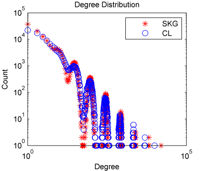
(a) Degree distribution

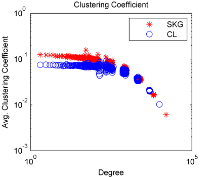
(b) Clustering coefficients

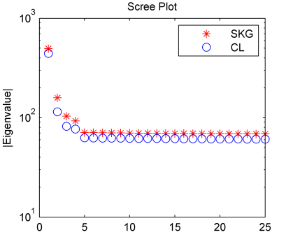
(c) Eigenvalues of adjacency matrices

(d) Assortativity

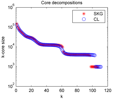
(e) Core decompositions

Figure 1: Comparison of the graph properties of SKG generated with Graph500 parameters and an equivalent CL.

1.4 Parameters for empirical study

We focus attention on the Graph500 benchmark [5]. This is primarily for concreteness and the relative importance of this parameter setting. Our results hold for all the settings of parameters that we experimented with. For NSKG, there is an additional noise parameter required. We set this to $0.1$, the setting studied in [21].

• Graph500: $T=[0.57,0.19;0.19,0.05]$, $\ell\in\{$26, 29, 32, 36, 39, 42$\}$, and $m=16\cdot 2^{\ell}$. We focus on a much smaller setting, $\ell=18$.

2 Previous Work

The SKG model was proposed by Leskovec et al. [23], as a generalization of the R-MAT model, given by Chakrabarti et al. [4]. Algorithms to fit SKG to real data were given by Leskovec and Faloutsos [2] (extended in [3]). This model has been chosen for the Graph500 benchmark [5]. Kim and Leskovec [24] defined a variant of SKG called the Multiplicative Attribute Graph (MAG) model.

There have been various analyses of the SKG model. The original paper [3] provides some basic theorems and empirically shows a variety of properties. Groër et al. [25], Mahdian and Xu [26], and Seshadhri et al. [21] study how the model parameters affect the graph properties. It has been conclusively shown that SKG cannot generate power-law distributions [21]. Seshadhri et al. also proposed noisy SKG (NSKG), which can provably produce lognormal degree distributions.

Sala et al. [27] perform an extensive empirical study of properties of graph models, including SKGs. Miller et al. [28] give algorithms to detect anomalies embedded in an SKG. Moreno et al. [29] study the distributional properties of families of SKGs.

A good survey of the edge-configuration model and its variants is given by Newman [30] (refer to Section IV.B). The specific model of CL was first given by Chung and Lu [17, 18]. They proved many properties of these graphs. Properties of its eigenvalues were given by Mihail and Papadimitriou [31] and Chung et al. [32].

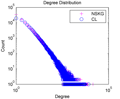
(a) Degree distribution

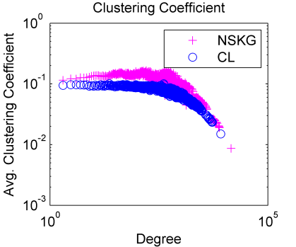
(b) Clustering coefficients

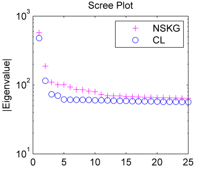
(c) Eigenvalues of adjacency matrices

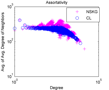
(d) Assortativity

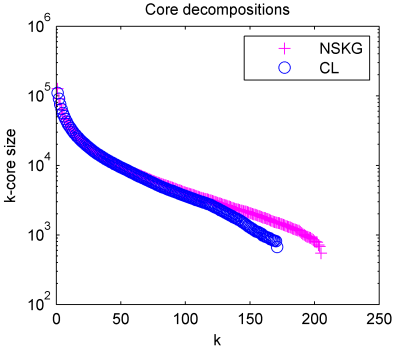
(e) Core decompositions

Figure 2: The figures compares the graph properties of NSKG generated with Graph500 parameters and an equivalent CL.

3 Similarity between SKG and CL

Our first experiment details the similarities between an SKG and its equivalent CL. We construct an SKG using the Graph500 parameters with $\ell=18$. We take the degree distribution of this graph, and construct a CL graph using this. Various properties of these graphs are given in Fig. 1. We give details below:

1. Degree distribution (Fig. 1a): This is the standard degree distribution plot in log-log scale. It is no surprise that the degree distributions are almost identical. After all, the weighting of CL is done precisely to match this.

2. Clustering coefficients (Fig. 1b): The clustering coefficient of a vertex $i$ is the fraction of wedges centered at $i$ that participate in triangles. We plot $d$ versus the average clustering coefficient of a degree $d$ vertex in log-log scale. Observe the close similarity. Indeed, we measure the difference between clustering coefficient values at $d$ to be at most $0.04$ (a lower order term with respect to commonly measured values in real graphs [33]).

3. Eigenvalues (Fig. 1c): Here, we plot the first 25 eigenvalues (in absolute value) of the adjacency matrix of the graph in log-scale. The proximity of eigenvalues is very striking. This is a strong suggestion that graph structure of the SKG and CL graphs are very similar.

4. Assortativity (Fig. 1d): This is non-standard measure, but we feel that it provides a lot of structural intuition. Social networks are often seen to be assortative [34, 35], which means that vertex of similar degree tend to be connected by edges. For $d$, define $X_{d}$ to be the average degree of an average degree $d$ vertex. We plot $d$ versus $X_{d}$ in log-log scale. Note that neither SKG nor CL are particularly assortative, and the plots match rather well.

5. Core decompositions (Fig. 1e): The $k$-cores of a graph are a very important part of understanding the community structure of a graph. The size of the $k$-core is the largest induced subgraph where each vertex has a minimum degree of $k$. This is a subset $S$ of vertices such that all vertices have $k$ neighbors in $S$. These sizes can be quickly determined by performing a core decomposition. This is obtained by iteratively deleting the minimum degree vertex of the graph. The core plots look amazingly close, and the only difference is that there are slightly larger cores in CL.

All these plots clearly suggest that the Graph500 SKG and its equivalent CL graph are incredibly close in their graph properties. Indeed, it appears that most important structural properties (especially from a social networks perspective) are closely related. We will show in §6 that CL performs an adequate job of fitting real data, and is quite comparable to SKG. We feel that any uses of SKG for benchmarking or test instances generation could probably be done with CL graphs as well.

For completeness, we plot the same comparisons between NSKG and CL in Fig. 2. We note again that the properties are very similar, though NSKG shows more variance in its values. Clustering coefficient values differ by at most $0.02$ here, and barring small differences in initial eigenvalues, there is a very close match. The assortativity plots show more oscillations for NSKG, but CL gets the overall trajectory.

4 Connection between SKG and CL matrices

Is there a principled explanation for the similarity observed in Fig. 1? It appears to be much more than a coincidence, considering the wide variety of graph properties that match. In this section, we provide an explanation based on the similarity of the probability matrices $P_{\textrm{SKG}}$ and $P_{\textrm{CL}}$. On analyzing these matrices, we see that they have an extremely close distribution of values. These matrices are themselves so fundamentally similar, providing more evidence that SKG itself can be modeled as CL.

We begin by giving precise formulae for the entries of the SKG and CL matrices. This is by no means new (or even difficult), but it should introduce the reader to the structure of these matrices. The vertices of the graph are labeled from $[n]$ (the set of positive integers up to $n$). For any $i$, ${\bf v}_{i}$ denotes the binary representation of $i$ as an $\ell$-bit vector. For two vectors ${\bf v}_{i}$ and ${\bf v}_{j}$, the number of common zeroes is the number of positions where both vectors are $0$. The following formula for the SKG entries has already been used in [4, 23, 25]. Observe that these entries (for both SKG and CL) are quite easy to compute and enumerate.

Claim 4.1

Let $i,j\in[n]$. Let the number of zeroes in ${\bf v}_{i}$ and ${\bf v}_{j}$ be $z_{i}$ and $z_{j}$ respectively. Let the number of common zeroes be $c_{z}$. Then

$$P_{\textrm{SKG}}(i,j)=t_{1}^{c_{z}}t_{2}^{z_{i}-c_{z}}t_{3}^{z_{j}-c_{z}}t_{4}^{\ell-z_{i}-z_{j}+c_{z}},\text{ and}$$

$$P_{\textrm{CL}}(i,j)\!=\!(t_{1}+t_{2})^{z_{i}}(t_{3}+t_{4})^{\ell-z_{i}}(t_{1}+t_{3})^{z_{j}}(t_{2}+t_{4})^{\ell-z_{j}}.$$

• The number of positions where ${\bf v}_{i}$ is zero but ${\bf v}_{j}$ is one is $z_{i}-c_{z}$. Analogously, the number of positions where only ${\bf v}_{j}$ is zero is $z_{j}-c_{z}$. The number of common ones is $\ell-z_{i}-z_{j}+c_{z}$. Hence, the $(i,j)$ entry of the $P_{\textrm{SKG}}$ is $t_{1}^{c_{z}}t_{2}^{z_{i}-c_{z}}t_{3}^{z_{j}-c_{z}}t_{4}^{\ell-z_{i}-z_{j}+c_{z}}$.

  Let us now compute the $(i,j)$ entry in the corresponding CL matrix. The probability that a single edge insertion becomes an out-edge of vertex $i$ in SKG is $(t_{1}+t_{2})^{z_{i}}(t_{3}+t_{4})^{\ell-z_{i}}$. Hence, the expected out-degree of $i$ is $m(t_{1}+t_{2})^{z_{i}}(t_{3}+t_{4})^{\ell-z_{i}}$. Similarly, the expected in-degree of $j$ is $m(t_{1}+t_{3})^{z_{j}}(t_{2}+t_{4})^{\ell-z_{j}}$. The $(i,j)$ entry of $P_{\textrm{CL}}$ is $(t_{1}+t_{2})^{z_{i}}(t_{3}+t_{4})^{\ell-z_{i}}(t_{1}+t_{3})^{z_{j}}(t_{2}+t_{4})^{\ell-z_{j}}.\hfill\Box$

The inspiration for this section comes from Fig. 3. Our initial aim was to understand the SKG matrix, and see whether the structure of the values provides insight into the properties of SKG. Since each entry in this probability matrix is of the form $t_{1}^{c_{z}}t_{2}^{z_{i}-c_{z}}t_{3}^{z_{j}-c_{z}}t_{4}^{\ell-z_{i}-z_{j}+c_{z}}$, there are many repeated values in this matrix. For each value in this probability matrix, we simply plot the number of times (the multiplicity) this value appears in the matrix. (For $P_{\textrm{SKG}}$, this is given in red) This is done for the associated $P_{\textrm{CL}}$ in blue. Note the uncanny similarity of the overall shapes for SKG and CL. Clearly, $P_{\textrm{SKG}}$ has more distinct values, but they are distributed fairly similarly to $P_{\textrm{CL}}$. Nonetheless, this picture is not very formally convincing, since it only shows the overall behavior of the distribution of values.

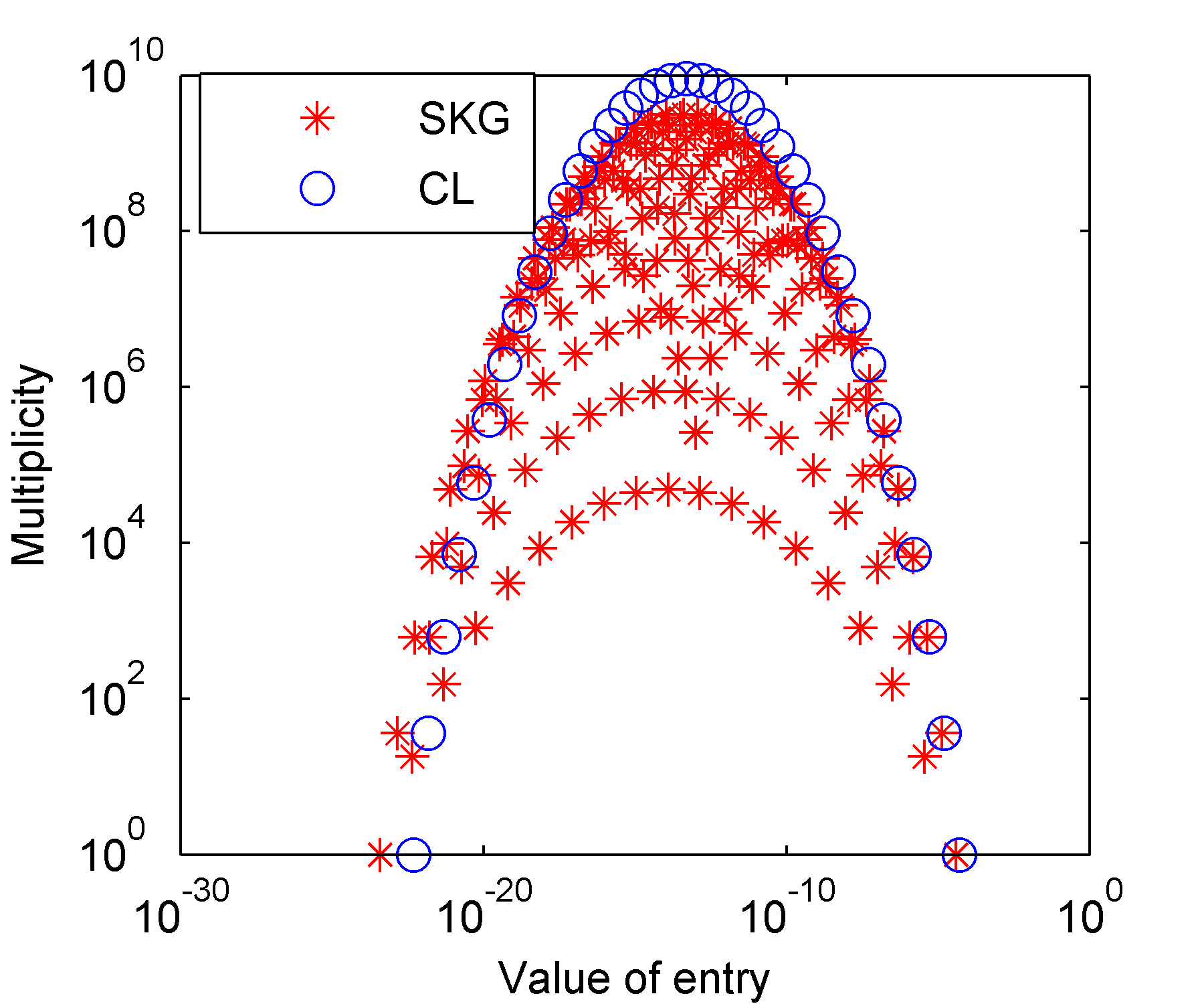
Figure 3: Distribution of entries of $P_{\textrm{SKG}}$ and $P_{\textrm{CL}}$.

Fig. 4 makes a more faithful comparison between the $P_{\textrm{SKG}}$ and $P_{\textrm{CL}}$ matrices. As we note from Fig. 3, $P_{\textrm{CL}}$ has a much smaller set of distinct entries. Suppose the distinct values in $P_{\textrm{CL}}$ are $v_{1}>v_{2}>v_{3}\ldots$. Associate a bin with each distinct entry of $P_{\textrm{CL}}$. For each entry of $P_{\textrm{SKG}}$, place it in the bin corresponding to the entry of $P_{\textrm{CL}}$ with the closest value. So, if some entry in $P_{\textrm{SKG}}$ has value $v$, we determine the index $i$ such that $|v-v_{i}|$ is minimized. This entry is placed in the $i$th bin. We can now look at the size of each bin for $P_{\textrm{SKG}}$. The size of the $i$th bin for the $P_{\textrm{CL}}$ is simply the multiplicity of $v_{i}$ in $P_{\textrm{CL}}$.

Observe how these sizes are practically identical for large enough entry value. Indeed the former portion of these plots, for value $<10^{-20}$, only accounts for a total of $<10^{-5}$ of the probability mass. This means that the fraction of edges that will correspond to these entries is at most $10^{-5}$. We can also argue that these entries correspond only to edges joining very low degree vertices to each other. In other words, the portion where these curves differ is really immaterial to the structure of the final graph generated.

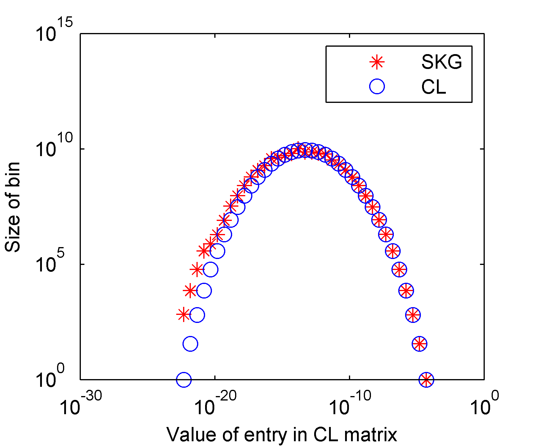
Figure 4: Bin sizes for $P_{\textrm{SKG}}$ and $P_{\textrm{CL}}$

This is very strong evidence that SKG behaves like a CL model. The structure of the matrices are extremely similar to each other. Fig. 5 is even more convincing. Now, instead of just looking at the size of each bin, we look at the total probability mass of each bin. For $P_{\textrm{SKG}}$ matrix, this is the sum of entries in a particular bin. For $P_{\textrm{CL}}$, this is the product of the size of the bin and the value (which is the again just the sum of entries in that bin). Again, we note the almost exact coincidence of these plots in the regime where the probabilities matter. Not only are the number of entries in each bin (roughly) the same, so is the total probability mass in the bin.

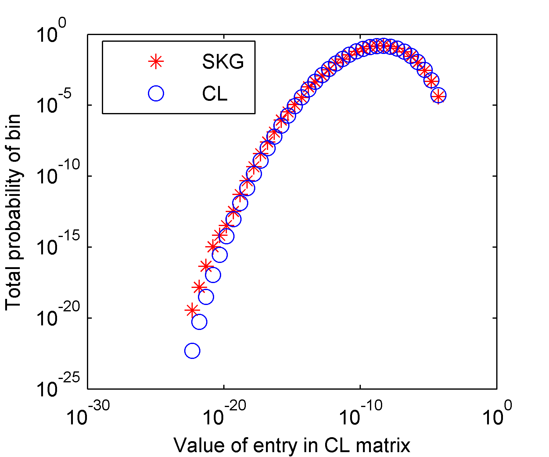
Figure 5: Probability mass of the bins

We now generate a random sample from $P_{\textrm{SKG}}$ and one from $P_{\textrm{CL}}$. Fig. 6 shows MATLAB spy plots of the corresponding graphs (represented by their adjacency matrices). One of the motivations for the SKG model was that it had a fractal or self-similar structure. It appears that the CL graph shares the same self-similarity. Furthermore, this self-repetition looks identical for the both SKG and CL graphs.

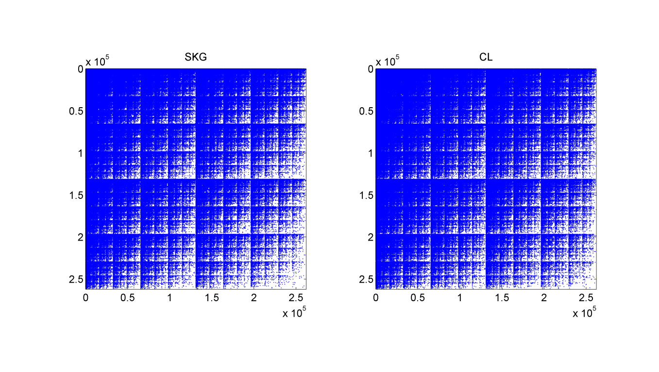
Figure 6: Spy plots of SKG drawn from $P_{\textrm{SKG}}$ and CL graph drawn from $P_{\textrm{CL}}$

5 Mathematical justifications

We prove that when the entries of the matrix $T$ satisfy the condition $t_{1}/t_{2}=t_{3}/t_{4}$, then SKG is identical to the CL model.

Theorem 5.1

Consider an SKG model where $T$ satisfies the following:

$$\frac{t_{1}}{t_{2}}=\frac{t_{3}}{t_{4}}.$$

Then $P_{\textrm{SKG}}=P_{\textrm{CL}}$.

• Let $\alpha=t_{1}/t_{2}=t_{3}/t_{4}$, and let $t_{3}=\beta t_{2}$. Then, $t_{1}=\alpha^{2}\beta t_{4}$; $t_{3}=\alpha\beta t_{2}$; and $t_{2}=\alpha t_{4}$. Note that since $t_{1}+t_{2}+t_{3}+t_{4}=1$,

  (5.1) $$(\alpha^{2}\beta+\alpha+\alpha\beta+1)t_{4}=1$$

  We use the formula given in Claim 4.1 for the $(i,j)$ entry of the SKG and CL matrices.

  By simple substitution, the entry for SKG is

  (5.2) $$(t_{4}\alpha^{2}\beta)^{c_{z}}(t_{4}\alpha)^{z_{i}-c_{z}}(t_{4}\alpha\beta)^{z_{j}-c_{z}}{t_{4}}^{\ell-z_{i}-z_{j}+c_{z}}$$

  $$= t^{\ell}_{4}\alpha^{z_{i}+z_{j}}\beta^{z_{j}}$$

  Analogously, for the CL matrix, the entry has value

  $$(t_{1}+t_{2})^{z_{i}}(t_{3}+t_{4})^{\ell-z_{i}}(t_{1}+t_{3})^{z_{j}}(t_{2}+t_{4})^{\ell-z_{j}}$$

  $$= [t_{4}(\alpha^{2}\beta+\alpha)]^{z_{i}}[t_{4}(\alpha\beta+1)]^{\ell-z_{i}}\times$$

  $$[t_{4}(\alpha^{2}\beta+\alpha\beta)]^{z_{j}}[\alpha(\alpha+1)]^{\ell-z_{j}}$$

  $$= t^{2\ell}_{4}(\alpha^{2}\beta\!+\!\alpha)^{z_{i}}(\alpha\beta\!+\!1)^{\ell-z_{i}}(\alpha^{2}\beta\!+\!\alpha\beta)^{z_{j}}(\alpha\!+\!1)^{\ell-z_{j}}$$

  $$= t^{2\ell}_{4}\alpha^{z_{i}+z_{j}}\beta^{z_{j}}(\alpha\beta+1)^{z_{i}}(\alpha\beta+1)^{\ell-z_{i}}\times$$

  $$(\alpha+1)^{z_{j}}(\alpha+1)^{\ell-z_{j}}$$

  $$= t^{2\ell}_{4}\alpha^{z_{i}+z_{j}}\beta^{z_{j}}(\alpha^{2}\beta+\alpha+\alpha\beta+1)^{\ell}$$

  $$= t^{\ell}_{4}\alpha^{z_{i}+z_{j}}\beta^{z_{j}}[t_{4}(\alpha^{2}\beta+\alpha+\alpha\beta+1)]^{\ell}$$

  $$= t^{\ell}_{4}\alpha^{z_{i}+z_{j}}\beta^{z_{j}}$$

  The last part follows from (5.1). This is exactly the same as (5.2). $\hfill\Box$

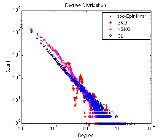
(a) Degree distribution

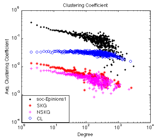
(b) Clustering coefficients

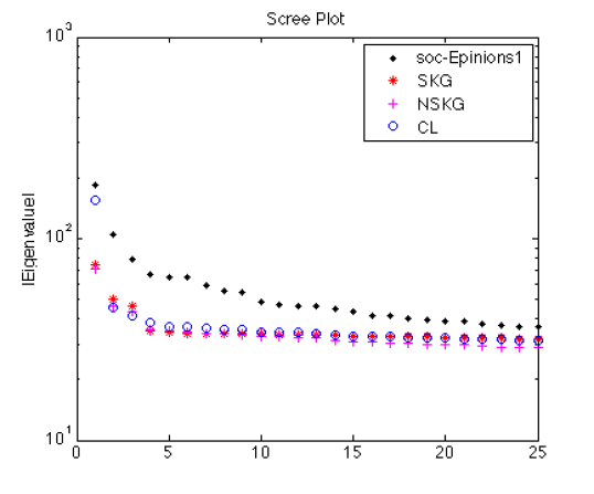
(c) Eigenvalues of adjacency matrices

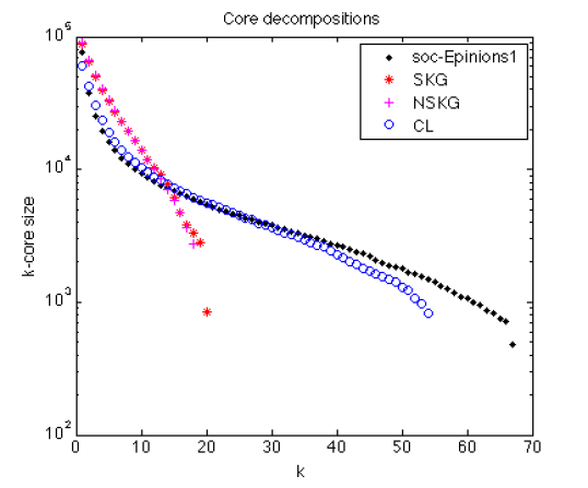
(d) Core decompositions

Figure 7: The figure compares the fits of various models for the social network soc-Epinions.

6 Fitting SKG vs CL

Fitting procedures for SKG model have been given in [3]. This is often cited as a reason for the popularity of SKG. These fits are based on algorithms for maximizing likelihood, but can take a significant amount of time to run. The CL model is fit by simply taking the degree distribution of the original graph. Note that the CL model uses a lot more parameters than SKG, which only requires $5$ independent numbers. In that sense, SKG is a very appealing model regardless of any other deficiencies.

We show comparisons of the CL, SKG, and NSKG models with respect to three different real graphs. For directed graphs, we look at the undirected version where directions are removed from all the edges. The real graphs are the following:

• soc-Epinions: This is a social network from the Epinions website, which tracks the “who-trusts-whom” relationship [36]. It has 75879 vertices and 811480 edges. The SKG parameters for this graph from [3] are: $T=[0.4668\ 0.2486;0.2243\ 0.0603]$, $\ell=17$.

• ca-HepTh: This is a co-authorship network from high energy physics [36]. It has 9875 vertices and 51946 edges. The SKG parameters for this graph from [3] are: $T=[0.469455\ 0.127350;0.127350\ 0.275846]$, $\ell=14$.

• cit-HepPh: This is a citation network from high energy physics [36]. It has 34546 vertices and 841754 edges. The SKG parameters from [3] are: $T=[0.429559\ 0.189715;0.153414\ 0.227312]$, $\ell=15$.

The comparisons between the properties are given, respectively, in Fig. 7, Fig. 8, and Fig. 9. In all of these, we see that CL (as expected) gives good fits to the degree distributions. For soc-Epinions, we see in Fig. 7a that the oscillations of the SKG degree distribution and how NSKG smoothens it out. Observe that the clustering coefficients of all the models are completely off. Indeed, for low degree vertices, the values are off by orders of magnitude. Clearly, no model is capturing the abundance of triangles in these graphs. The eigenvalues of the model graphs are also distant from the real graph, but CL performs no worse than SKG (or NSKG). Core decompositions for soc-Epinions (Fig. 7d) show that CL fits rather well. For ca-HepPh (Fig. 8d) CL is marginally better than SKG, whereas for cit-HepTh (Fig. 9d), NSKG seems be a better match.

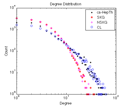
(a) Degree distribution

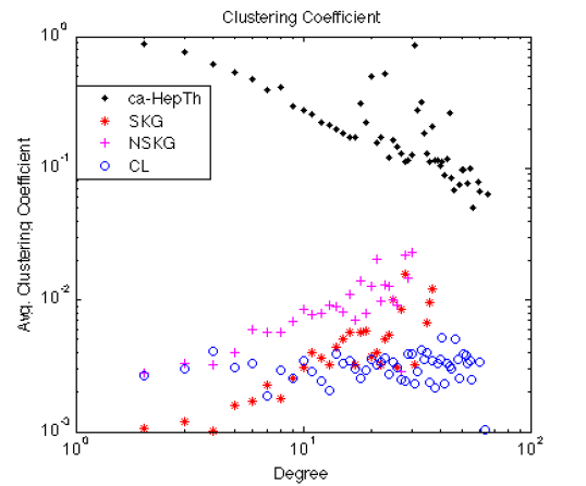
(b) Clustering coefficients

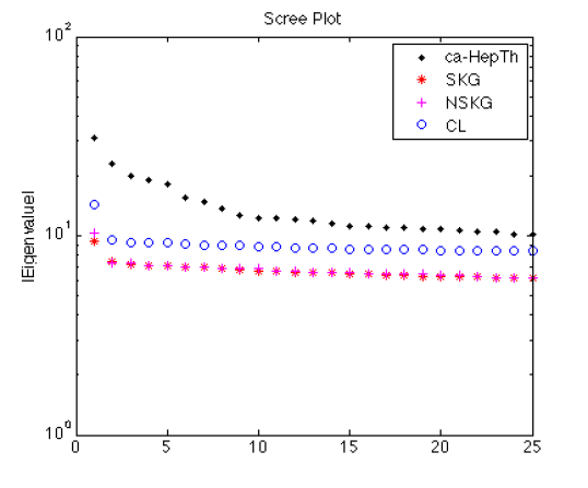
(c) Eigenvalues of adjacency matrices

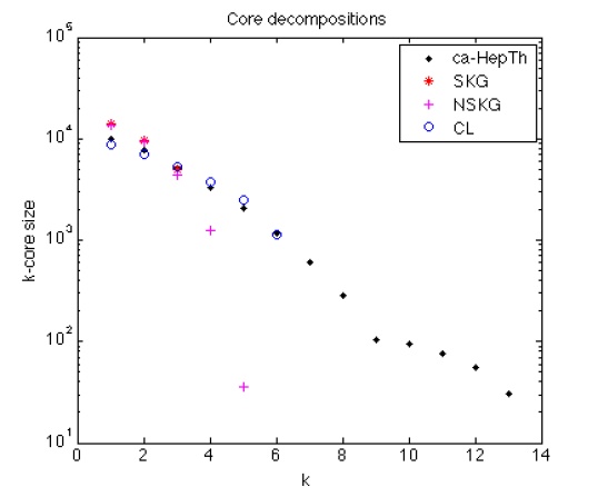
(d) Core decompositions

Figure 8: The figures compares the fits of various models for the co-authorship network ca-HepTh.

All in all, there is no conclusive evidence that SKG or NSKG model these graphs significantly better than CL. We feel that the comparable performance of CL shows that it should be used as a control model to compare against.

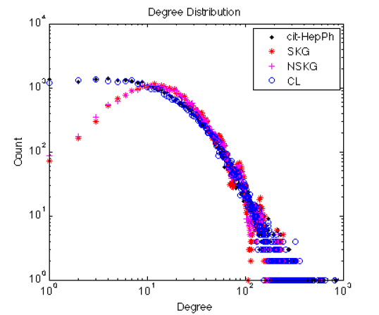
(a) Degree distribution

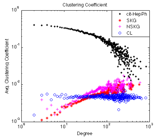
(b) Clustering coefficients

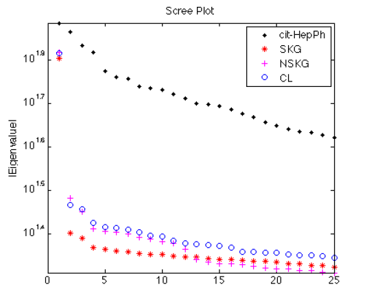
(c) Eigenvalues of adjacency matrices

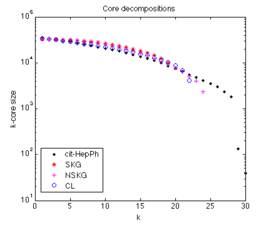
(d) Core decompositions

Figure 9: The figures compares the fits of various models for the citation network cit-HepPh.

7 Conclusions

Understanding existing graph models is a very important part of graph analysis. We need to clearly see the benefits and shortcomings of existing models, so that we can use them more effectively. For these purposes, it is good to have a simple “baseline” model to compare against. We feel that the CL model is quite suited for this because of its efficiency, simplicity, and similarity to SKG. Especially for benchmarking purposes, it is a good candidate for generating simple test graphs. One should not think of this as representing real data, but as an easy way of creating reasonable looking graphs. Comparisons with the CL model can give more insight into current models. The similarities and differences may help identify how current graph models differ from each other.

References

- [1] D. Chakrabarti and C. Faloutsos, “Graph mining: Laws, generators, and algorithms,” ACM Computing Surveys, vol. 38, no. 1, 2006.
- [2] J. Leskovec and C. Faloutsos, “Scalable modeling of real graphs using Kronecker multiplication,” in ICML ’07. ACM, 2007, pp. 497–504.
- [3] J. Leskovec, D. Chakrabarti, J. Kleinberg, C. Faloutsos, and Z. Ghahramani, “Kronecker graphs: An approach to modeling networks,” J. Machine Learning Research, vol. 11, pp. 985–1042, Feb. 2010. [Online]. Available: http://jmlr.csail.mit.edu/papers/v11/leskovec10a.html
- [4] D. Chakrabarti, Y. Zhan, and C. Faloutsos, “R-MAT: A recursive model for graph mining,” in SDM ’04, 2004, pp. 442–446. [Online]. Available: http://siam.org/proceedings/datamining/2004/dm04_043chakrabartid.pdf
- [5] Graph 500 Steering Committee, “Graph 500 benchmark,” 2010, available at http://www.graph500.org/Specifications.html.
- [6] V. Vineet, P. Harish, S. Patidar, and P. J. Narayanan, “Fast minimum spanning tree for large graphs on the gpu,” in Proceedings of the Conference on High Performance Graphics 2009, ser. HPG ’09. New York, NY, USA: ACM, 2009, pp. 167–171. [Online]. Available: http://doi.acm.org/10.1145/1572769.1572796
- [7] N. Edmonds, T. Hoefler, and A. Lumsdaine, “A space-efficient parallel algorithm for computing betweenness centrality in distributed memory,” in High Performance Computing (HiPC), 2010 International Conference on, dec. 2010, pp. 1 –10.
- [8] R. Pearce, M. Gokhale, and N. M. Amato, “Multithreaded asynchronous graph traversal for in-memory and semi-external memory,” in Proceedings of the 2010 ACM/IEEE International Conference for High Performance Computing, Networking, Storage and Analysis, ser. SC ’10. Washington, DC, USA: IEEE Computer Society, 2010, pp. 1–11. [Online]. Available: http://dx.doi.org/10.1109/SC.2010.34
- [9] A. Buluç and J. R. Gilbert, “Highly parallel sparse matrix-matrix multiplication,” CoRR, vol. abs/1006.2183, 2010.
- [10] M. Patwary, A. Gebremedhin, and A. Pothen, “New multithreaded ordering and coloring algorithms for multicore architectures,” in Euro-Par 2011 Parallel Processing, ser. Lecture Notes in Computer Science, E. Jeannot, R. Namyst, and J. Roman, Eds. Springer Berlin / Heidelberg, 2011, vol. 6853, pp. 250–262.
- [11] S. Hong, T. Oguntebi, and K. Olukotun, “Efficient parallel graph exploration on multi-core cpu and gpu,” in Proc. Parallel Architectures and Compilation Techniques(PACT), 2011.
- [12] S. J. Plimpton and K. D. Devine, “MapReduce in MPI for large-scale graph algorithms,” Parallel Computing, vol. 37, no. 9, pp. 610 – 632, 2011, emerging Programming Paradigms for Large-Scale Scientific Computing. [Online]. Available: http://www.sciencedirect.com/science/article/pii/S0167819111000172
- [13] D. Bader and K. Madduri, “Snap, small-world network analysis and partitioning: An open-source parallel graph framework for the exploration of large-scale networks,” in Parallel and Distributed Processing, 2008. IPDPS 2008. IEEE International Symposium on, april 2008, pp. 1 –12.
- [14] B. Hendrickson and J. Berry, “Graph analysis with high-performance computing,” Computing in Science Engineering, vol. 10, no. 2, pp. 14 –19, march-april 2008.
- [15] M. C. Schmidt, N. F. Samatova, K. Thomas, and B.-H. Park, “A scalable, parallel algorithm for maximal clique enumeration,” Journal of Parallel and Distributed Computing, vol. 69, no. 4, pp. 417 – 428, 2009. [Online]. Available: http://www.sciencedirect.com/science/article/pii/S0743731509000082
- [16] W. Aiello, F. Chung, and L. Lu, “A random graph model for power law graphs,” Experimental Mathematics, vol. 10, pp. 53–66, 2001.
- [17] F. Chung and L. Lu, “The average distances in random graphs with given expected degrees,” Proceedings of the National Academy of Sciences USA, vol. 99, pp. 15 879–15 882, 2002.
- [18] ——, “Connected components in random graphs with given degree sequences,” Annals of Combinatorics, vol. 6, pp. 125–145, 2002.
- [19] P. Erdös and A. Rényi, “On random graphs,” Publicationes Mathematicae, vol. 6, pp. 290–297, 1959.
- [20] ——, “On the evolution of random graphs,” Publications of the Mathematical Institute of the Hungarian Academy of Sciences, vol. 5, pp. 17–61, 1960.
- [21] C. Seshadhri, A. Pinar, and T. Kolda, “An in-depth analysis of stochastic kronecker graphs,” in Proc. ICDM 2011, IEEE Int. Conf. Data Mining, 2011, to appear.
- [22] ——, “An in-depth analysis of stochastic kronecker graphs,” September 2011, arxiv:1102.5046. [Online]. Available: http://arxiv.org/abs/1102.5046
- [23] J. Leskovec, D. Chakrabarti, J. Kleinberg, and C. Faloutsos, “Realistic, mathematically tractable graph generation and evolution, using Kronecker multiplication,” in PKDD 2005. Springer, 2005, pp. 133–145.
- [24] M. Kim and J. Leskovec, “Multiplicative attribute graph model of real-world networks,” in WAW 2010, 2010, pp. 62–73.
- [25] C. Groër, B. D. Sullivan, and S. Poole, “A mathematical analysis of the R-MAT random graph generator,” Jul. 2010, available at http://www.ornl.gov/~b7r/Papers/rmat.pdf.
- [26] M. Mahdian and Y. Xu, “Stochastic Kronecker graphs,” Random Structures & Algorithms, vol. 38, no. 4, pp. 453–466, 2011.
- [27] A. Sala, L. Cao, C. Wilson, R. Zablit, H. Zheng, and B. Y. Zhao, “Measurement-calibrated graph models for social network experiments,” in WWW ’10. ACM, 2010, pp. 861–870.
- [28] B. Miller, N. Bliss, and P. Wolfe, “Subgraph detection using eigenvector L1 norms,” in NIPS 2010, 2010, pp. 1633–1641. [Online]. Available: http://books.nips.cc/papers/files/nips23/NIPS2010_0954.pdf
- [29] S. Moreno, S. Kirshner, J. Neville, and S. V. N. Vishwanathan, “Tied Kronecker product graph models to capture variance in network populations,” in Proc. 48th Annual Allerton Conf. on Communication, Control, and Computing, Oct. 2010, pp. 1137–1144.
- [30] M. E. J. Newman, “The structure and function of complex networks,” SIAM Review, vol. 45, no. 2, pp. 167–256, 2003.
- [31] C. Papadimitriou and M. Mihail, “On the eigenvalue power law,” in RANDOM, 2002, pp. 254–262.
- [32] F. Chung, L. Lu, and V. Vu, “Eigenvalues of random power law graphs,” Annals of Combinatorics, vol. 7, pp. 21–33, 2003.
- [33] M. Girvan and M. Newman, “Community structure in social and biological networks,” Proceedings of the National Academy of Sciences, vol. 99, pp. 7821–7826, 2002.
- [34] M. E. J. Newman, “Mixing patterns in networks,” Phys. Rev. E., vol. 67, p. 026126, Feb. 04 2002. [Online]. Available: http://arxiv.org/abs/cond-mat/0209450
- [35] ——, “Assortative mixing in networks,” Phys. Rev. Letter, vol. 89, p. 208701, May 20 2002. [Online]. Available: http://arxiv.org/abs/cond-mat/0205405
- [36] Stanford Network Analysis Project (SNAP), available at http://snap.stanford.edu/.