Profile shape stability and phase jitter analyses of millisecond pulsars

Abstract

Millisecond pulsars (MSPs) have been studied in detail since their discovery in 1982. The integrated pulse profiles of MSPs appear to be stable, which enables precision monitoring of the pulse times of arrival (TOAs). However, for individual pulses the shape and arrival phase can vary dramatically, which is known as pulse jitter. In this paper, we investigate the stability of integrated pulse profiles for 5 MSPs, and estimate the amount of jitter for PSR J0437$-$4715. We do not detect intrinsic profile shape variation based on integration times from $\sim 10$ to $\sim 100$ s with the provided instrumental sensitivity. For PSR J0437$-$4715 we calculate the jitter parameter to be $f_{J}=0.067\pm 0.002$, and demonstrate that the result is not significantly affected by instrumental TOA uncertainties. Jitter noise is also found to be independent of observing frequency and bandwidth around 1.4 GHz on frequency scales of $<100$ MHz, which supports the idea that pulses within narrow frequency scale are equally jittered. In addition, we point out that pulse jitter would limit TOA calculation for the timing observations with future telescopes like the Square Kilometre Array and the Five hundred metre Aperture Spherical Telescope. A quantitative understanding of pulse profile stability and the contribution of jitter would enable improved TOA calculations, which are essential for the ongoing endeavours in pulsar timing, such as the detection of the stochastic gravitational wave background.

1 Introduction

Millisecond pulsars (MSPs) have been shown to exhibit highly stable rotational behaviour (e.g. Verbiest et al., 2009). They are a vital tool in investigating the physical environment of the pulsars, via precise monitoring of pulse times of arrival (TOAs), the so-called pulsar timing technique. Previous work using precision pulsar timing has already yielded tests of General Relativity in the strong field regime (e.g. Taylor & Weisberg, 1989; Kramer et al., 2006), improvements of neutron star equation of state models (e.g. Lattimer & Prakash, 2007; Demorest et al., 2010; Özel et al., 2010), and studies of the interstellar medium (ISM) structure (e.g. You et al., 2007). Via pulsar timing arrays (PTAs), upper bounds have already been placed on the stochastic gravitational wave background (Jenet et al., 2006; van Haasteren et al., 2011; Yardley et al., 2011). The next generation of radio telescopes (such as the Five hundred metre Aperture Spherical Telescope, FAST and the Square Kilometre Array, SKA) will significantly improve upon the available instrumental sensitivity allowing timing to much higher precision and for many more sources. This tremendous advance in hardware will significantly increase the sensitivity of future PTAs and allow more detailed studies of the gravitational wave background, such as its polarisation and speed of propagation (Lee et al., 2008; Lee et al., 2010). Individual gravitational wave sources, such as supermassive black hole binaries at the centre of galaxies can also be identified via a future PTA study (e.g. Lee et al., 2011; Sesana et al., 2011).

The extreme timing precision required to reach the aforementioned scientific goals is more readily achievable with MSPs because of their short spin periods, their regular rotational behaviour and, last but not least, their greatly stable average pulse shapes. In general, single pulses from a pulsar show significant shape modulation. Up to now, several types of variable behaviour have been observed within the population of pulsars. These include intrinsic pulse-to-pulse changes caused by random phase jitter of individual pulses (Cordes & Downs, 1985; Cordes, 1993), systematic position changes of sub-components named “sub-pulse drifting” (e.g. Drake & Craft, 1968; Cordes, 1975; Edwards & Stappers, 2003), switching between two or more profile shapes on both short and long timescales known as “mode-changing” (e.g. Cordes et al., 1978; Ferguson et al., 1981; Lyne et al., 2010), and state changes of intrinsic flux density mentioned as “nulling” (e.g. Backer, 1970; Wang et al., 2007). Studies of bright individual pulses from MSPs have shown only the first type of pulse-to-pulse variation (Cognard et al., 1996; Jenet et al., 1998), which can cause fluctuation in the phase of integrated profiles and introduce TOA uncertainty in addition to the radiometer noise (Cordes & Shannon, 2010). This is the effect mainly addressed within the framework of this paper.

Statistically, as the single pulses are clearly unstable, shape differences are expected to exist between an integrated profile over a short integration time and a standard template formed by averaging many more pulses. Note that the shape difference, if sufficiently large, would influence the accuracy of TOA estimation by the standard cross-correlation approach (Liu et al., 2011). Consequently, it is important to evaluate whether or not the shape mismatch is significant compared with the system noise level. There have already been studies investigating the shape correlation between integrated profiles (or even single pulses) and a pre-formed template (Helfand et al., 1975; Rankin & Rathnasree, 1995; Jenet et al., 1998; Jenet et al., 2001). The results show clear shape difference for young pulsars and a less significant or even undetectable difference for MSPs with the given sensitivity.

If the TOA uncertainties can be shown to be mostly due to radiometer noise and phase jitter, based on an assumed model, the amount of jitter can be estimated from timing on a short timescale and such analysis has already been carried out for PSR J1713+0747 (Cordes & Shannon, 2010). The result can be used both for the error analysis in timing and as an input for jittered shape correction approaches (Messenger et al., 2011; Oslowski et al., 2011).

The structure of this paper is as follows. In Section 2 we introduce the approach used for evaluating profile stability and jitter estimation. The observations, instruments and data pre-processing techniques used are described in Section 3. In Section 4 we present the results before drawing our conclusions in Section 5.

2 Profile shape and pulse jitter analysis

2.1 Stability Analysis

The shape and phase instability of single pulses will induce shape modulation for integrated profiles, which can be mitigated by increasing the number of pulses added. The similarity between an observed integrated profile $p$ and a normalised standard shape $s$, obtained from previous observations, is simply evaluated by the correlation coefficient $\rho$, which is defined as:

$$\rho=\frac{\displaystyle\sum_{i}(s_{i}-\bar{s})(p_{i}-\bar{p})}{\displaystyle\sqrt{\sum_{i}(s_{i}-\bar{s})^{2}}\sqrt{\sum_{i}(p_{i}-\bar{p})^{2}}},$$ (1)

where $i$ stands for the sample number of the data points across the profile. It is shown in Appendix A that, assuming an identical intrinsic shape for the observed profile and standard, there is a scaling law between $\rho$ and the profile peak signal-to-noise ratio (SNR, defined as pulse peak amplitude divided by root-mean-square of the noise) of: $(1-\rho)\propto\rm SNR^{-2}$. Note that this power law is followed only in the high SNR regime (e.g. for SNR$\gtrsim 20$). From the scaling law, we define a shape constant, $\mathfrak{C}$, related only to the intrinsic profile shape as:

$$\mathfrak{C}\equiv{\rm SNR}\cdot\sqrt{1-\rho}\simeq\left(\frac{n_{\rm samp}}{\displaystyle 2\sum_{i}(s_{i}-\bar{s})^{2}}\right)^{1/2},$$ (2)

where $n_{\rm samp}$ is the number of time samples of a profile and $i=1,2,\cdots n_{\rm samp}$. Once the SNR and $\rho$ are measured, respectively, the shape constant can then be determined and used to compare with the value calculated directly from the waveform of the standard.

If the profile integration increases the SNR as expected as $\rm SNR\propto\sqrt{N}$, where $N$ is number of pulses folded, then we reach the relation between $N$ and $\rho$ as: $(1-\rho)\propto N^{-1}$. However, the scaling is not obeyed if the SNR varies significantly from pulse to pulse, which can be caused by intrinsic flux variation, system temperature changes and diffractive scintillation. So in our analysis we use the effective pulse number $N_{\rm efc}$, the number of pulses weighted by SNR to account for the variation of the profile SNR which does indeed scales as $\rm SNR\propto\sqrt{N_{\rm efc}}$ and hence $1-\rho\propto N^{-1}_{\rm efc}$ (Liu et al., 2011).

2.2 Phase Jitter

Single pulse instability can also cause TOA fluctuations of integrated profiles. This phase jitter could, in principle, be investigated directly from single pulse data, although the sensitivity achieved by the current instruments may not enable sufficient SNR for carrying out the study on all pulses within a narrow band. Another approach is to perform timing using integrated profiles on short timescales and to estimate the amount of jitter from the timing residuals. As a first-order approximation, by assuming an identical shape for single pulses and a Gaussian-distributed central phase probability, the contribution of pulse jitter to the uncertainty of TOA can be calculated as in Cordes & Shannon (2010). In brief, the measurement error of TOAs on short timescales (e.g. several hours) can be summarised as:

$$\sigma_{\rm total}^{2}=\sigma_{\rm rn}^{2}+\sigma_{\rm J}^{2}+\sigma_{\rm scint}^{2}+\sigma^{2}_{0},$$ (3)

where $\sigma_{\rm rn}$, $\sigma_{\rm J}$, $\sigma_{\rm scint}$ and $\sigma_{0}$ correspond to uncertainty induced by radiometer noise, pulse jitter, instability of short-term diffractive scintillation, and all other possible contributions (faults in timing model, instrumental digitisation artefacts, polarisation calibration error, etc), respectively. Following Downs & Reichley (1983), Cordes et al. (1990) and Cordes & Shannon (2010), we have

$$\sigma_{\rm rn}^{2} = \frac{\Delta}{N\times SNR_{1}^{2}\int[U^{\prime}(t)]^{2}dt},$$ (4)

$$\sigma_{\rm J}^{2} = f_{J}^{2}\frac{\int U(t)t^{2}dt}{N\int U(t)dt},$$ (5)

$$\sigma_{\rm scint}^{2} = \frac{t^{2}_{\rm d}}{N_{\rm scint}}.$$ (6)

Here $N$ is the number of pulses, $SNR_{1}$ is the signal-to-noise ratio for a single pulse, $U(t)$ is the profile waveform, $\Delta$ is the sampling time, $f_{J}$ is the width of the Gaussian probability of single pulse phase in units of the pulse width, $t_{\rm d}$ is the pulse broadening timescale, and $N_{\rm scint}$ is the number of scintles contained by the integration. We can see that the ratio of $\sigma_{\rm rn}$ to $\sigma_{\rm J}$ is proportional to the equivalent single pulse SNR. The value of $SNR_{1}$ for MSPs, based on current observations, is mostly far less than unity, leading to the case where the white noise term is dominant in TOA uncertainty. However, the contribution by phase jitter will become more significant when timing is carried out by the next generation of radio telescopes, which will have a significant improvement in sensitivity of $1-2$ orders of magnitude over current systems (Nan, 2006; Schilizzi et al., 2007; Liu et al., 2011). In this case, TOA error prediction based solely on radiometer noise will be incorrect.

The statistics of the timing residuals which are obtained by subtracting a timing model from the measured TOAs, can be evaluated via a reduced $\chi^{2}$ value given by

$$\chi^{2}_{\rm rec}=\frac{1}{N-n-1}\chi^{2}=\frac{1}{N-n-1}\sum_{i}\left(\frac{\Delta x_{i}}{\sigma_{i}}\right)^{2},$$ (7)

where $N$ is the number of residuals, $n$ is the number of fitted parameters, and $\Delta x_{i}$, $\sigma_{i}$ are the $i$th residual and its corresponding measurement error, respectively. Normally, $\sigma_{i}$ accounts for only the uncertainty of radiometer noise $\sigma_{\rm rn}$ in Eq. (4), which can be obtained from the template matching technique (Taylor, 1992). Theoretically, if the timing residuals are dominated by radiometer noise, a timing solution with residuals of $\chi^{2}_{\rm rec}\simeq 1$ will be expected. The existence of other types of noise would make the $\sigma_{i}$ underestimated and deviate $\chi^{2}_{\rm rec}$ from unity. The contribution from the diffractive scintillation can be estimated by Eq. (6). Here $t_{\rm d}$ can be obtained from the NE2001 Galactic Free electron Density Model (Cordes & Lazio, 2002), and the number of scintles is assessable via either a dynamic spectrum or more detailed calculations in Cordes et al. (1990). If the additional noise is mostly from pulse jitter, one can estimate the jitter noise $\sigma_{J}$ by adding its contribution into $\sigma_{i}$ to have $\chi^{2}_{\rm rec}=1$. Accordingly, the value of the jitter parameter $f_{J}$ can be derived based on Eq. (5), and the probability density distribution of $f_{J}$ can be calculated from the standard $\chi^{2}$ distribution, given by

$$f(x;k)=\frac{1}{2^{k/2}\Gamma(k/2)}x^{k/2-1}e^{-x/2},$$ (8)

where $x$ is the $\chi^{2}$ value and $k=N-n-1$ is the degrees of freedom.

3 Observations

Table 1: Details of observations used in this paper. The symbols $t_{0}$, $N_{0}$ and $T_{\rm obs}$ represent the shortest integration time in the dataset, the number of time dumps and the observational length, respectively. The asterisk (*) denotes that the data were pre-processed by the DFB and the others are from CPSR2.

Pulsar Name	MJD	Receiver	$t_{0}$ (s)	$N_{0}$	$T_{\rm obs}$ (hr)
J0437$-$4715	53576	MB	16.7772	1595	8.7
	53621	MB	16.7772	1498	8.9
	53864	MB	67.1088	261	6.9
	$54095^{*}$	H-OH	60.0017	125	2.4
	54222	H-OH	67.1088	135	9.8
	54226	H-OH	67.1088	152	8.9
J1022+1001	53260	MB	16.7772	114	0.5
J1603$-$7202	53166	H-OH	16.8099	114	0.5
J1713+0747	53221	H-OH	16.7771	215	3.3
J1730$-$2304	53145	H-OH	16.7772	114	0.5

Frequent observations, typically weekly, of more than 20 MSPs are performed at the Parkes 64-m radio telescope (Verbiest et al., 2009). Here we use the data from five sources (PSR J0437$-$4715, PSR J1022+1001, PSR J1603$-$7202, PSR J1713+0747, PSR J1730$-$2304), collected using either the Parkes 20-cm multibeam (MB) receiver (Staveley-Smith et al., 1996) or the ‘H-OH’ receiver. The data were processed online with the Caltech-Parkes-Swinburne Recorder 2 (CPSR2), a 2-bit coherent de-disperser back-end that records two 64-MHz wide observing bands simultaneously (Hotan et al., 2006). These bands were centred at observing frequencies of 1341 and 1405 MHz, respectively. Data collected before MJDs 53740 were folded every 16.7772 s, and after that every 67.1088 s. Off-source observations of a pulsed noise probe at 45^∘ to the feed probes, but with otherwise identical set-up, were taken at regular intervals for the purpose of polarimetric calibration. Additionally, we analysed data for PSR J0437$-$4715 from the new Parkes Digital Filterbank (DFB) system, a digital polyphase filterbank capable of 8-bit sampling. In Table 1 we present the details for all selected datasets.

The data were then pre-processed with the psrchive software package (Hotan et al., 2004). Specifically, for CPSR2 data we corrected the 2-bit digitisation artefact (Jenet & Anderson, 1998) by applying the algorithm in van Straten (in preparation), and removed 12.5 % of each edge of the bandpass to avoid possible effects of aliasing and spectral leakage. A full receiver model was determined and applied to perform the polarisation calibration to the MB receiver data (van Straten, 2004), as the receiver suffers from strong cross-coupling between the orthogonal feeds. For the H-OH data from both back-ends we used the common single-axis model instead, as the coupling was found to be an order of magnitude weaker (e.g. Manchester et al., 2010). The signals from each polarisation were summed into total power (Stokes $I$), while 0.5 MHz frequency channels were kept for later analysis purposes. The template profiles used for the correlation coefficient calculation and the cross-correlation procedure to estimate $\sigma_{\rm rn}$ (Taylor, 1992), were obtained independently from the datasets shown in Table 1. All CPSR2 datasets have passed through the test shown in Liu et al. (2011) to ensure no significant 2-bit digitisation distortion is present. The test also showed that the template matching produced the radiometer noise uncertainty as expected by Eq. (4).

4 Results

4.1 Measurement of shape constant

The measurement of the shape constant for individual integrations gives an estimate of the profile stability, which here we have carried out for the aforementioned five MSPs. For PSR J0437$-$4715, $\mathfrak{C}$ was determined using the the first 500 time dumps of the MJD 53621 dataset. For PSRs J1022+1001 and J1730$-$2304 we integrated the time dumps into 1.0 and 1.8 minutes, separately, so as to obtain sufficiently high SNR for calculation of $\mathfrak{C}$ and statistical analysis (see e.g. Fig. 8). The $\rho$ is computed with respect to the on-pulse phase and the root-mean-square (RMS) deviation of the noise is estimated based on the off-pulse region, from which one can derive the value of $\mathfrak{C}$ from Eq. (2). The expected values of $\mathfrak{C}$ (denoted by $\mathfrak{C}_{0}$) are calculated directly from the shape of the high SNR standards formed from previous observations, which are also used in the calculations of $\rho$. The errors in $\rho$ and the RMS of the baseline of the profile are given by Eq. (17) and by $\simeq{\rm RMS}/\sqrt{2n_{\rm samp}}$, respectively.

We present the shape constant measurement of PSR J0437$-$4715 for the MJD 53621 dataset in Fig. 1 as an example, and show the statistical result in Table 2. It is clear that for most sources, within the range of estimated error the measured $\mathfrak{C}$ is in accordance with the analytical value. The RMS of the measured value also matches the mean error bar for each data point. The deviation of the measured $\mathfrak{C}$ from the expectation for PSR 1730$-$2304 may indicate an intrinsic level of profile shape change, but could also be due to an insufficient number of measurements. Note that, in this case, the statistics are only based on 13 data points, while for each of the others more than 30 measurements were available.

It is worth noting that there has already been previous work regarding the stability of PSR J1022+1001 on both short and long timescales, with inconclusive results (Kramer et al., 1999; Ramachandran & Kramer, 2003; Hotan et al., 2004). On timescales of roughly an hour, our results do not show profile changes. However, the analysis was carried out using the whole on-pulse phase, and may not be sensitive to variations occurring only around the profile peaks. Any shape variations, if they exist, are likely to affect mostly the peaks. A detailed analysis of the statistics of the peak ratios will be published by Purver et al. (in preparation).

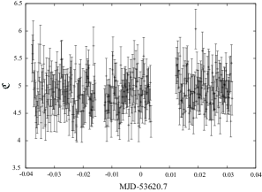
Figure 1: Shape constant measurements for the first 500 integrations of the MJD 53621 observation for PSR J0437$-$4715. The time baseline of these measurements is $\sim 1.9$ hours.

Table 2: Statistical results of the profile shape constant measurement for all five sources. The parameters $t_{\rm int}$, $\mathfrak{C}_{0}$, $\overline{\mathfrak{C}}$, RMS, $\overline{\sigma}$ and $k_{\rm NC}$ represent integration time of the integrated profiles, shape constant calculated from the standard, mean of measured $\mathfrak{C}$, RMS of measurements, mean of individual measurement errors, and the fitted slopes of $N_{\rm efc}$ versus $(1-\rho)$ curves in Fig. 2, respectively.

Pulsar Name	$t_{\rm int}$ (s)	$\mathfrak{C}_{0}$	$\overline{\mathfrak{C}}$	RMS	$\overline{\sigma}$	$k_{\rm NC}$
J0437$-$4715	16.8	4.8	4.9	0.32	0.31	-1.00(1)
J1022+1001	67.1	2.7	2.6	0.22	0.20	-0.98(1)
J1603$-$7202	16.8	3.9	4.0	0.33	0.30	-0.99(1)
J1713+0747	16.8	3.7	3.8	0.23	0.22	-0.94(2)
J1730$-$2304	117	2.9	3.2	0.24	0.27	-0.98(1)

To investigate the scaling relation indicated by Eq. (2), for each source we perform incremental integrations along the dataset, adding more pulse periods each time. Our results are presented in Fig. 2 which shows the relation between the weighted number of integrated pulses and $\rho$. It is clear that all curves are linear in log-log space for the $N_{\rm efc}-(1-\rho)$ relation as expected. The fitted slopes all lie in the range of (0.94, 1.00), as given in the last column of Table 2. This result, together with the $\mathfrak{C}$ statistics in Table 2, indicates no detectable profile shape variation along the integration.

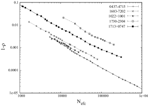
Figure 2: $N_{\rm efc}-(1-\rho)$ plot for all five sources. The effective pulse number is used to compensate for the varied weight of each integration due to the difference in SNR. All curves show expected linear behavior with fitted slopes to $-1$ in log-log space.

4.2 Fit of phase jitter

Estimation of the jitter parameter $f_{J}$ can be performed only on the brightest source PSR J0437$-$4715, as single pulse SNR for the other sources is not high enough and radiometer noise is still dominant in the timing residuals. Here we use all PSR J0437$-$4715 datasets listed in Table 1, each of which contains over a hundred individual integrations to yield a stable statistical result. When performing the timing of the datasets, we used the timing models derived by Verbiest et al. (2009). TOAs and their uncertainties were determined through cross-correlation with a pre-formed standard, individually for each side of band. No EFAC or EQUAD value were applied to change the measurement precision as done commonly in timing analysis (e.g. van Haasteren et al., 2011).

The timing solution of PSR J0437$-$4715 shows a widely scattered series of TOAs over a timescale of several hours, with a reduced $\chi^{2}$ far larger than unity, which strongly indicates the existence of extra uncertainty contributions besides radiometer noise. Fig. 3 shows the timing residuals of the MJD 53621 dataset for the 1405 MHz band. The TOAs were produced by summing over the whole bandwidth of effectively 48 MHz, yielding reduced $\chi^{2}$ values of 8.45 and 8.46 for the 1341 MHz and the 1405 MHz side band, respectively. Note that from Eq. (6), the TOA fluctuation induced by unstable profile broadening due to the ISM is approximately the scattering timescale once the observational bandwidth is much narrower than the scintillation frequency scale (thus $N_{\rm scint}\simeq 1$). For PSR J0437$-$4715, as the scintillation bandwidth and pulse broadening time are $\approx 0.4$ GHz and $\approx 1$ ns (Cordes & Lazio, 2002), respectively, this uncertainty is negligible for the datasets used in this paper.

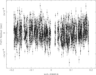
Figure 3: The short-term timing solution of PSR J0437$-$4715 over $\sim$8 hours dataset on MJD 53621 at a central frequency of 1405 MHz with 48 MHz bandwidth.

Following the method mentioned in Section 2.2, we measure $f_{J}$ based on the shortest integrations from all PSR J0437$-$4715 datasets in Table 1, and the results are summarised in Table 3. It is clear that the measurements from datasets collected by different receivers are consistent with each other. This does not indicate significant uncertainty contribution by polarimetric calibration error. Results from two types of back-end also show consistency after correcting for the bias induced by low-frequency noise of the CPSR2 data (see the next paragraph for details). Additionally, the same result for fits from both sides of the band suggests that the intensity of phase jitter does not vary significantly on small frequency scales (there is a 64 MHz difference between the two bands) at observing frequencies around 1.4 GHz. The combination of all measurements for both sides of the band achieves an estimated $f_{J}$ of $0.067\pm 0.002$. To study the statistics of the residuals, we perform Kolmogorov-Smirnov (K-S) tests on each dataset, on TOAs weighted by the modified uncertainties accounting for phase jitter. The measured p-values (e.g. Press et al., 1986) are summarised in Table 3, not suggesting a significant deviation of the weighted residuals from a Gaussian distribution. This demonstrates the dominance of Gaussian noise in the residuals.

Table 3: Results of jitter parameter $f_{J}$ measurements and K-S tests of all PSR J0437$-$4715 datasets from two 48-MHz sub-bands. The parameters $f$ and $\mathcal{P}$ represent the central frequency and the p-value of K-S test, respectively.

Dataset (MJD)	$f$ (MHz)	$f_{J}$	$\mathcal{P}$
53576	1341	$0.067\pm 0.004$	0.89
	1450	$0.067\pm 0.004$	0.93
53621	1341	$0.067\pm 0.004$	0.98
	1405	$0.066\pm 0.004$	0.62
53964	1341	$0.066\pm 0.004$	0.88
	1405	$0.065\pm 0.004$	0.92
54095	1341	$0.069\pm 0.006$	0.90
	1405	$0.073\pm 0.006$	0.92
54222	1341	$0.069\pm 0.007$	0.52
	1405	$0.067\pm 0.007$	0.77
54226	1341	$0.068\pm 0.005$	0.20
	1405	$0.066\pm 0.006$	0.64

To investigate the dependence of the result on the length of individual integrations, we calculate the weighted RMS against integration time $t_{\rm int}$ for multiple combinations of instruments. In detail, MJD 53576 (CPSR2+MB), MJD 54095 (DFB+H-OH) and MJD 54226 (CPSR2+H-OH) datasets are chosen to demonstrate different hardware configurations, and the results are shown in Fig. 4. Clearly, the curves yielded by CPSR2 data collected by two receivers are consistent, again implying no significant contribution of timing uncertainty by polarisation calibration. The relation obtained from DFB data achieves a fitted slope close to $-0.5$, supporting the idea from Eq. (3) that timing residual scales as the square-root of the number of integrated pulses once only the uncertainties by radiometer noise and jitter are significant. The residuals from the CPSR2 data coincide with those from the DFB in 1-min integrations, and then saturate at the level of $\approx$150 ns as the integration time is extended. This implies that the difference may be due to different digitisation procedures. The saturation corresponds to additional self-correlated noise which contributes $\approx$8% bias in our $f_{J}$ measurement based on 1-min integrations of CPSR2 data, which has been corrected for in the results of Table 3.

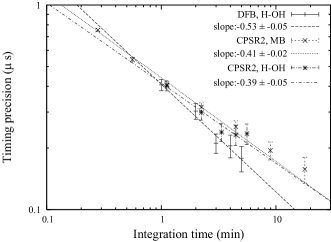
Figure 4: Weighted timing residual versus integration time relation for three combinations of instruments. The curve yielded by the DFB data shows the expected power law with an index close to $-0.5$, while the curves from CPSR2 data clearly deviate from this, which implies additional uncertainty perhaps due to the low-bit digitisation procedure.

The expression for $\sigma_{\rm J}$ indicates that the uncertainty due to jitter is independent of the observational bandwidth and central frequency. To illustrate this, the MJD 53621 dataset is divided into two, three, four and six sub-bands each time. Then a fit for the jitter parameter is carried out individually on each sub-band and the results are combined incoherently to obtain an estimated value of $f_{J}$ for a given bandwidth. The procedure is carried out on both side-bands and the result is shown in Fig. 5. It is clear that at both central frequencies jitter noise remains once the bandwidth is changed. The result indicates that, on small frequency scales, pulses are jittered in the same way, otherwise jitter noise would not remain the same after summing the entire bandwidth. In Fig. 6 we plot the fitted $f_{J}$ based on 8 MHz bandwidth against the central frequency for each sub-band. The group of $f_{J}$ values do not show a clear dependence on the observational frequency, and yield average, weighted RMS and reduced $\chi^{2}$ of 0.069, 0.006 and 1.1, respectively. The mean correlation coefficient between residuals of different sub-bands were calculated to be $\simeq 0.51$, which indicates a correlation among the time series and supports the idea of equal jittering on small frequency scales.

Figure 5: Fitted amount of jitter against chosen bandwidth for both sides of band from MJD 53621 dataset. No clear dependency between these two parameters is visible.

Figure 6: Estimated jitter parameter based on an 8-MHz sub-bands from the MJD 53621 dataset. The $f_{J}$ shows no clear trend of evolution across a frequency range of $\sim 100$ MHz.

5 Conclusions and Discussions

5.1 Summary of the results

In this paper, we investigate the issue of MSP profile stability based on five pulsars in total. A shape constant associated with the correlation coefficient is defined to quantify the stability. No significant shape modulation of integrated profiles beyond the measurement error is found for integration times from $10^{1}$ to $10^{2}$ s. For PSR J0437$-$4715 we estimate the jitter parameter by performing timing on short timescales and comparing the actual timing residual with the amount expected from radiometer noise. The fitted $f_{J}$ is found to be consistent on both sides of the bands (64 MHz difference in central frequency), and the combination of several datasets results in an estimate of $0.067\pm 0.002$. It is also demonstrated that all the other potential sources of TOA uncertainty, besides radiometer and jitter noise, do not strongly influence the measurement. Additionally, we show that jitter noise scales neither with bandwidth within a 50-MHz band nor with frequency across a range of $\sim 100$ MHz at 1.4 GHz, which supports the idea that pulses are equally jittered on small frequency scales. Such results, if still valid for wider frequency range, would suggest that the jittering uncertainty cannot be mitigated by extending the observing bandwidth (also see Oslowski et al., 2011).

5.2 Future telescopes

Apart from bright single pulses and giant pulses (e.g. Cognard et al., 1996; Jenet et al., 1998), pulse jitter of the majority of MSP pulses is still not detectable with currently available sensitivity. However, with the next generation of radio telescopes, the shape modulation of integrated profiles for some of the bright MSPs will become visible. In Fig. 7, based on the aforementioned jitter model and assuming $f_{J}=0.1$, we perform a Monte Carlo simulation to calculate the relation between the number of integrated pulses and $1-\rho$ for the case of jitter only, and compare the result with the curves from considering radiometer noise only for a few instruments. We assume a 5-ms period, a 100-$\mu$s pulse width, and a 5-mJy flux density at 1.4 GHz for a sample MSP, and 1.4 GHz frequency with 300 MHz bandwidth for observation. The gains of FAST and SKA are assumed to be $20$ $\rm m^{2}/K$ and $100$ $\rm m^{2}/K$, respectively (Nan, 2006; Schilizzi et al., 2007). For the assumed jitter model the scaling also follows $1-\rho\propto N^{-1}$ as calculated in Appendix B. It is shown that an SKA observation of an MSP of typical brightness, pulse jitter is comparable to radiometer noise in influencing the correlation-coefficient value. Note that in the applied jitter model all single pulses are assumed to be identical, so the simulated jitter curve can potentially move upwards once the shape modulation is also accounted for. Future observations with the SKA of PSR J0437$-$4715 will be totally dominated by pulse jitter in shape variation, so it will be ideal for single pulse study.

Once the shape variation of integrated profiles by pulse jitter becomes significant, the current cross-correlation method for the measurement of TOAs would fail in estimating the TOA uncertainty correctly. Specifically, the model in the template-matching procedure now needs to be of the form (Taylor, 1992):

$$P(t)=A_{0}*S(t)+n(t)+j(t),$$ (9)

where $P(t)$ is the observed profile, $S(t)$ is the template, and $n(t)$ is the noise function. The parameter $j(t)$ is the jitter-induced shape perturbation, which, referring to MSPs, is mostly negligible compared with $n(t)$ for the current sensitivity. If this shape difference becomes sufficiently large, the calculated TOA precision would fail to follow the expected SNR scaling (Liu et al., 2011). In this case, the shape modulation would need to be modelled (e.g., by principal component analysis, see Cordes & Shannon, 2010; Oslowski et al., 2011) and then a global determination of the unknown parameters could be performed to properly estimate the TOA (e.g. Messenger et al., 2011).

Figure 7: $1-\rho$ versus $N$ curve prediction of PSR J0437$-$4715 for different instruments and simulation. The pulses are created with identical shape and a jitter parameter of $f_{J}=0.1$ is used to simulate the Gaussian-distributed phase variation.

Appendix A Correlation-coefficient Scaling for Additive Noise

Assume the observed profile is a superposition of a normalised template $\rm\bf p$ and Gaussian noises $\rm\bf n$, i.e. $p_{i}=s_{i}+n_{i}$. The subscript $i$ goes from $1$ to $n$, the number of the profile bins. We regard $\rm\bf p$ and $\rm\bf n$ as $n$-dimensional vectors. Following Eq. (1), the correlation coefficient between the perfect template $\rm\bf s$ and observed profile $\rm\bf p$ is

$$\rho=\frac{\displaystyle\sum_{i}c_{i}(c_{i}+n_{i})}{\displaystyle\sqrt{\sum_{i}c^{2}_{i}\sum_{i}(c_{i}+n_{i})^{2}}}\,,$$ (10)

where $c_{i}=s_{i}-\bar{s}$.

Assume that the noise $\rm\bf n$ is a multivariate Gaussian with probability distribution $f({\rm\bf n})$ and covariance matrix $\rm\bf C$, where $C_{ij}=\sigma_{\rm n}^{2}\delta_{ij}$. The expectation value of correlation coefficient $\langle\rho\rangle$ and its second-order moment $\langle\rho^{2}\rangle$ are

$$\langle\rho\rangle = \int\rho f({\rm\bf n})\,d{\rm\bf n}$$ (11)

$$\langle\rho^{2}\rangle = \int\rho^{2}f({\rm\bf n})\,d{\rm\bf n}$$ (12)

The variance for $\rho$ is then $\sigma_{\rho}^{2}=\langle\rho^{2}\rangle-\langle\rho\rangle^{2}$. The Eq. (11) and (12) can be integrated by transforming into hyper-spherical coordinates (Mathews & Walker, 1970). Although no analytical expression could be found, by using asymptotic technique we derive the results for the case of a large sample number which match both the low and high SNR cases as below:

$$\displaystyle 1-\langle\rho\rangle = 1-\left(\frac{1}{1+\chi}\right)^{1/2}$$ (13)

$$= \displaystyle\left\{\begin{array}[]{cc}1-(\frac{1}{\chi})^{1/2}+{\cal O}\left(\frac{1}{\chi^{3/2}}\right),&\chi\gg 1\\ \displaystyle\frac{1}{2}\chi+{\cal O}\left(\chi^{2}\right),&\chi\ll 1\end{array}\right.$$ (16)

$$\sigma_{\rho}=\left\{\begin{array}[]{cc}\displaystyle\left[\frac{\chi}{n_{\rm samp}(1+\chi)}\right]^{1/2}+{\cal O}\left(\frac{1}{\chi^{2}}\right),&\chi\gg 1\\ \displaystyle\chi\left(\frac{n_{\rm samp}-1}{2n^{2}_{\rm samp}}\right)^{1/2}+{\cal O}\left(\chi^{2}\right.),&\chi\ll 1\end{array}\right.$$ (17)

where

$$\chi=\frac{\displaystyle\sigma_{\rm n}^{2}}{\displaystyle\overline{\sum_{i}c_{i}^{2}}},~{}~{}~{}~{}\overline{\sum_{i}c_{i}^{2}}=\frac{\displaystyle\sum_{i}c_{i}^{2}}{n_{\rm samp}}.$$ (18)

In Fig. 8 a set of Monte Carlo simulations are performed so as to test the validity of the derivation. Here a simple Gaussian template shape is assumed and profiles are created by adding normal distributed noise onto the template. It can be seen that for most SNR ranges the results from both approaches coincide with each other, and for high SNR value, $1-\rho$ scales linearly with the increase of signal.

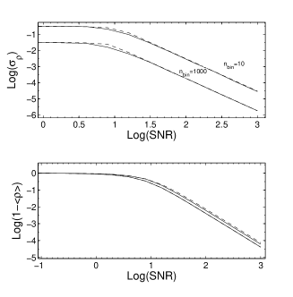
Figure 8: Theoretical and simulated results presenting the relation between SNR and correlation factors. In each case the dashed line represents the analytic solution and the solid line stands for the numerical result. The parameter $n_{\rm bin}$ is the number of segments for the profiles.

Appendix B Correlation-coefficient Scaling for Jitter

In this section, we prove that the relation $1-\langle\rho\rangle\propto 1/N$. Assuming single pulses are of identical waveform $p_{0}(\phi)$ and the effect of phase jitter is to introduce a random phase to each single pulse, i.e. the $i$-th single pulse takes a waveform of $p_{0}(\phi+\Delta\phi_{i})$, where the $\Delta\phi_{i}$ is a random phase. The waveform of the template profile $p(\phi)$ is defined by summing infinite number of single pulses as

$$p(\phi)=\lim_{N\to\infty}\frac{1}{N}\sum_{i=1}^{N}p_{0}(\phi+\Delta\phi_{i})\,.$$ (19)

Meanwhile, an integrated profile $p_{N}$ obtained from an observational session is yielded by averaging $N$ single pulses ($N\gg 1$) as

$$p_{\rm N}(\phi)=\frac{1}{N}\sum_{i=1}^{N}p_{0}(\phi+\Delta\phi_{i})\,.$$ (20)

The correlation coefficient between the template $p(\phi)$ and $N$-averaged integrated pulse profile $p_{N}(\phi)$ is then

$$\rho=\frac{\displaystyle\int_{0}^{1}{p(\phi)}p_{N}(\phi)\,d\phi}{\left[\displaystyle{\int_{0}^{1}{p(\phi)}^{2}\,d\phi\int_{0}^{1}p_{N}(\phi)^{2}\,d\phi}\right]^{\frac{1}{2}}}\,,$$ (21)

The evaluation for the statistical expectation of correlation coefficient is already presented in Cordes & Shannon (2010). In this appendix, a slightly different approach is applied. Letting

$$\delta(\phi)=p_{N}(\phi)-p(\phi)\,,$$ (22)

we have

$$\rho=\frac{\int_{0}^{1}p^{2}(\phi)+p(\phi)\delta(\phi)\,d\phi}{\left[\int_{0}^{1}p^{2}(\phi)\,d\phi\int_{0}^{1}p^{2}(\phi)+2p(\phi)\delta(\phi)+\delta^{2}(\phi)\,d\phi\right]^{\frac{1}{2}}}$$ (23)

Since the number of pulse in observations is usually large, we expect that the $p_{N}(\phi)$ is very close to $p(\phi)$, which leads to $\delta(\phi)\ll p(\phi)$. In this case, one can show that

$$\langle\rho\rangle=1+\frac{1}{2}\left\langle\left(\frac{\int_{0}^{1}p(\phi)\delta(\phi)\,d\phi}{\int_{0}^{1}p^{2}(\phi)\,d\phi}\right)^{2}-\frac{\int_{0}^{1}\delta^{2}(\phi)\,d\phi}{\int_{0}^{1}p^{2}(\phi)\,d\phi}\right\rangle+{\cal O}\left(\frac{\delta^{4}}{p_{0}^{4}}\right)\,,$$ (24)

which is equivalent to

$$\langle 1-\rho\rangle\simeq\frac{1}{2}\left\langle\frac{\int_{0}^{1}p_{N}^{2}(\phi)\,d\phi}{\int_{0}^{1}p^{2}(\phi)\,d\phi}-\left(\frac{\int_{0}^{1}p(\phi)p_{N}(\phi)\,d\phi}{\int_{0}^{1}p^{2}(\phi)\,d\phi}\right)^{2}\right\rangle\,.$$ (25)

To understand how the $1-\langle\rho\rangle$ depends on the number of pulses $N$, we have to expand $p_{N}(\phi)$ in the above equations. One can then have (Cordes & Shannon, 2010)

$$\left\langle\int_{0}^{1}p_{N}^{2}(\phi)\,d\phi\right\rangle = \frac{N^{2}-N}{N^{2}}\int_{0}^{1}p^{2}(\phi)\,d\phi$$ (26)

$$+\frac{1}{N}\int_{0}^{1}\langle p_{0}^{2}(\phi+\Delta\phi)\rangle\,d\phi\,,$$

and

$$\left\langle\left(\int_{0}^{1}p(\phi)p_{N}(\phi)\,d\phi\right)^{2}\right\rangle=\frac{N^{2}-N}{N^{2}}\int_{0}^{1}p^{2}(\phi)\,d\phi$$

$$+\frac{1}{N}\int_{0}^{2}\,d\phi\int_{0}^{1}\,d\phi^{\prime}p(\phi)p(\phi^{\prime})\langle p_{0}(\phi+\Delta\phi)p_{0}(\phi^{\prime}+\Delta\phi)\rangle\,.$$ (27)

Here we assume that the phase jitter is independent, i.e. $\langle\Delta\phi_{i}\Delta\phi_{j}\rangle=0$, if $i\neq j$. Thus

$$\langle 1-\rho\rangle=\frac{1}{2N}\left[S-K\right]\,$$ (28)

where

$$S = \frac{\int_{0}^{1}\langle p_{0}^{2}(\phi+\Delta\phi)\rangle\,d\phi}{\int_{0}^{1}p^{2}(\phi)\,d\phi}\,,$$ (29)

$$K = \frac{\int_{0}^{2}\,d\phi\int_{0}^{1}\,d\phi^{\prime}p(\phi)p(\phi^{\prime})\langle p_{0}(\phi+\Delta\phi)p_{0}(\phi^{\prime}+\Delta\phi)\rangle}{\left(\int_{0}^{1}p^{2}(\phi)\,d\phi\right)^{2}}\,.$$

Because neither $S$ nor $K$ is $N$-dependant, the Eq. (28) clearly show the scaling relation that $1-\langle\rho\rangle\propto 1/N$.

We also further compare the result of $1-\langle\rho\rangle$ form Monte Carlo simulations and from the Eq. (28) in the Fig. 9. Clearly, the numerical simulation and analytical calculation match each other at larger $N$ limit as we expected.

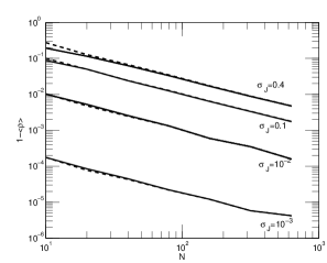
Figure 9: The $1-\langle\rho\rangle$ as function of $N$ and $\sigma_{\rm J}$, where $\sigma^{2}_{\rm J}$ is the variance of the phase jitter probability density function. The dashed lines are from analytical calculation, the Eq. (28), while the solid lines are from direct Monte Carlo simulations.

References

- Backer (1970) Backer D. C., 1970, Nature, 228, 42
- Cognard et al. (1996) Cognard I., Shrauner J. A., Taylor J. H., Thorsett S. E., 1996, ApJ, 457, L81
- Cordes (1975) Cordes J. M., 1975, ApJ, 195, 193
- Cordes (1993) Cordes J. M., 1993, in Phillips J. A., Thorsett S. E., Kulkarni S. R., ed, Planets around Pulsars. Astron. Soc. Pac. Conf. Ser. Vol. 36, p. 43
- Cordes & Downs (1985) Cordes J. M., Downs G. S., 1985, ApJS, 59, 343
- Cordes & Lazio (2002) Cordes J. M., Lazio T. J. W., arXiv:astro-ph/0207156
- Cordes et al. (1978) Cordes J. M., Rankin J. M., Backer D. C., 1978, ApJ, 223, 961
- Cordes & Shannon (2010) Cordes J. M., Shannon R. M., 2010, astro-ph/1107.3086
- Cordes et al. (1990) Cordes J. M., Wolszczan A., Dewey R. J., Blaskiewicz M., Stinebring D. R., 1990, ApJ, 349, 245
- Demorest et al. (2010) Demorest P. B., Pennucci T., Ransom S. M., Roberts M. S. E., Hessels J. W. T., 2010, Nature, 467, 1081
- Downs & Reichley (1983) Downs G. S., Reichley P. E., 1983, ApJS, 53, 169
- Drake & Craft (1968) Drake F. D., Craft H. D., 1968, Nature, 220, 231
- Edwards & Stappers (2003) Edwards R. T., Stappers B. W., 2003, A&A, 407, 273
- Ferguson et al. (1981) Ferguson D. C., Boriakoff V., Weisberg J. M., Backus P. R., Cordes J. M., 1981, A&A, 94, 16
- Helfand et al. (1975) Helfand D. J., Manchester R. N., Taylor J. H., 1975, ApJ, 198, 661
- Hotan et al. (2004) Hotan A. W., Bailes M., Ord S. M., 2004, MNRAS, 355, 941
- Hotan et al. (2006) Hotan A. W., Bailes M., Ord S. M., 2006, MNRAS, 369, 1502
- Hotan et al. (2004) Hotan A. W., van Straten W., Manchester R. N., 2004, PASA, 21, 302
- Jenet et al. (1998) Jenet F., Anderson S., Kaspi V., Prince T., Unwin S., 1998, ApJ, 498, 365
- Jenet & Anderson (1998) Jenet F. A., Anderson S. B., 1998, PASP, 110, 1467
- Jenet et al. (2001) Jenet F. A., Anderson S. B., Prince T. A., 2001, ApJ, 546, 394
- Jenet et al. (2006) Jenet F. A. et al., 2006, ApJ, 653, 1571
- Kramer et al. (2006) Kramer M. et al., 2006, Science, 314, 97
- Kramer et al. (1999) Kramer M., Xilouris K. M., Camilo F., Nice D., Lange C., Backer D. C., Doroshenko O., 1999, ApJ, 520, 324
- Lattimer & Prakash (2007) Lattimer J. M., Prakash M., 2007, Phys. Rep., 442, 109,165
- Lee et al. (2010) Lee K., Jenet F. A., Price R. H., Wex N., Kramer M., 2010, ApJ, 722, 1589
- Lee et al. (2008) Lee K. J., Jenet F. A., Price R. H., 2008, ApJ, 685, 1304
- Lee et al. (2011) Lee K. J., Wex N., Kramer M., Stappers B. W., Bassa C. G., Janssen G. H., Karuppusamy R., Smits R., 2011, MNRAS, 414, 3251
- Liu et al. (2011) Liu K., Verbiest J. P. W., Kramer M., Stappers B. W., van Straten W., Cordes J. M., 2011, MNRAS in press, astro-ph/1107.3086
- Lyne et al. (2010) Lyne A., Hobbs G., Kramer M., Stairs I., Stappers B., 2010, Science, 329, 408
- Manchester et al. (2010) Manchester R. N. et al., 2010, ApJ, 710, 1694
- Mathews & Walker (1970) Mathews J., Walker R. L., 1970, Mathematical methods of physics. Addison-Wesley World Student Series, Menlo Park, Ca.
- Messenger et al. (2011) Messenger C., Lommen A., Demorest P., Ransom S., 2011, Classical and Quantum Gravity, 28, 055001
- Nan (2006) Nan R., 2006, Science in China G: Physics and Astronomy, 49, 129
- Oslowski et al. (2011) Oslowski S., van Straten W., Hobbs G., Bailes M., Demorest P., 2011, MNRAS in press, astro-ph/1108.0812
- Özel et al. (2010) Özel F., Psaltis D., Ransom S., Demorest P., Alford M., 2010, ApJ, 724, L199
- Press et al. (1986) Press W. H., Flannery B. P., Teukolsky S. A., Vetterling W. T., 1986, Numerical Recipes: The Art of Scientific Computing. Cambridge University Press, Cambridge
- Ramachandran & Kramer (2003) Ramachandran R., Kramer M., 2003, A&A, 407, 1085
- Rankin & Rathnasree (1995) Rankin J. M., Rathnasree N., 1995, ApJ, 452, 814
- Schilizzi et al. (2007) Schilizzi R. T. et al., 2007, Preliminary specifications for the square kilometre array, Memo 100, SKA Program Development Office
- Sesana et al. (2011) Sesana A., Roedig C., Reynolds M. T., Dotti M., 2011, astro-ph/1107.2927
- Staveley-Smith et al. (1996) Staveley-Smith L., Manchester R. N., Tzioumis A. K., Reynolds J. E., Briggs D. S., 1996, in McCray R., Wang Z., ed, IAU Colloquium 145: Supernovae and supernova remnants. Cambridge University Press, p. 309
- Taylor (1992) Taylor J. H., 1992, Philos. Trans. Roy. Soc. London A, 341, 117
- Taylor & Weisberg (1989) Taylor J. H., Weisberg J. M., 1989, ApJ, 345, 434
- van Haasteren et al. (2011) van Haasteren R. et al., 2011, MNRAS, 414, 3117
- van Straten (2004) van Straten W., 2004, ApJ, 152, 129
- Verbiest et al. (2009) Verbiest J. P. W. et al., 2009, MNRAS, 400, 951
- Wang et al. (2007) Wang N., Manchester R. N., Johnston S., 2007, MNRAS, 377, 1383
- Yardley et al. (2011) Yardley D. R. B. et al., 2011, MNRAS, 414, 1777
- You et al. (2007) You X.-P. et al., 2007, MNRAS, 378, 493