Convex Hulls of Quadratically Parameterized Sets With Quadratic Constraints

Abstract

Let $V$ be a semialgebraic set parameterized as

$$\{(f_{1}(x),\ldots,f_{m}(x)):\,x\in T\}$$

for quadratic polynomials $f_{0},\ldots,f_{m}$ and a subset $T$ of $\mathbb{R}^{n}$. This paper studies semidefinite representation of the convex hull $\mbox{conv}(V)$ or its closure, i.e., describing $\mbox{conv}(V)$ by projections of spectrahedra (defined by linear matrix inequalities). When $T$ is defined by a single quadratic constraint, we prove that $\mbox{conv}(V)$ is equal to the first order moment type semidefinite relaxation of $V$, up to taking closures. Similar results hold when every $f_{i}$ is a quadratic form and $T$ is defined by two homogeneous (modulo constants) quadratic constraints, or when all $f_{i}$ are quadratic rational functions with a common denominator and $T$ is defined by a single quadratic constraint, under some general conditions.

Dedicated to Bill Helton on the occasion of his 65th birthday.

1 Introduction

A basic question in convex algebraic geometry is to find convex hulls of semialgebraic sets. A typical class of semialgebraic sets is parameterized by multivariate polynomial functions defined on some sets. Let $V\subset\mathbb{R}^{m}$ be a set parameterized as

$$V=\{(f_{1}(x),\ldots,f_{m}(x)):\,x\in T\}$$ (1.1)

with every $f_{i}(x)$ being a polynomial and $T$ a semialgebraic set in $\mathbb{R}^{n}$. We are interested in finding a representation for the convex hull $\mbox{conv}(V)$ of $V$ or its closure, based on $f_{1},\ldots,f_{m}$ and $T$. Since $V$ is semialgebraic, $\mbox{conv}(V)$ is a convex semialgebraic set. Thus, one wonders whether $\mbox{conv}(V)$ is representable by a spectrahedron or its projection, i.e., as a feasible set of semidefinite programming (SDP). A spectrahedron of $\mathbb{R}^{k}$ is a set defined by a linear matrix inequality (LMI) like

$$L_{0}+w_{1}L_{1}+\cdots+w_{k}L_{k}\succeq 0$$

for some constant symmetric matrices $L_{0},\ldots,L_{k}$. Here the notation $X\succeq 0$ (resp. $X\succ 0$) means the matrix $X$ is positive semidefinite (resp. definite). Equivalently, a spectrahedron is the intersection of a positive semidefinite cone and an affine linear subspace. Not every convex semialgebraic set is a spectrahedron, as found by Helton and Vinnikov [7]. Actually, they [7] proved a necessary condition called rigid convexity for a set to be a spectrahedron. They also proved that rigid convexity is sufficient in the two dimensional case. Typically, projections of spectrahedra are required in representing convex sets (if so, they are also called semidefinite representations). It has been found that a very general class of convex sets are representable as projections of spectrahedra, as shown in [4, 5]. The proofs used sum of squares (SOS) type representations of polynomials that are positive on compact semialgebraic sets, as given by Putinar [15] or Schmüdgen [16]. More recent work about semidefinite representations of convex semialgebraic sets can be found in [6, 9, 10, 11, 12].

A natural semidefinite relaxation for the convex hull $\mbox{conv}(V)$ can be obtained by using the moment approach [9, 13]. To describe it briefly, we consider the simple case that $n=1$, $T=\mathbb{R}$ and $(f_{1}(x),f_{2}(x),f_{3}(x))=(x^{2},x^{3},x^{4})$ with $m=3$. The most basic moment type semidefinite relaxation of $\mbox{conv}(V)$ in this case is

$$R=\left\{(y_{2},y_{3},y_{4}):\begin{bmatrix}1&y_{1}&y_{2}\\ y_{2}&y_{2}&y_{3}\\ y_{2}&y_{3}&y_{4}\end{bmatrix}\succeq 0\mbox{ for some }y_{1}\in\mathbb{R}\right\}.$$

The underlying idea is to replace each monomial $x^{i}$ by a lifting variable $y_{i}$ and to pose the LMI in the definition of $R$, which is due to the fact that

$$\begin{bmatrix}1\\ x\\ x^{2}\end{bmatrix}\begin{bmatrix}1\\ x\\ x^{2}\end{bmatrix}^{T}\quad=\quad\begin{bmatrix}1&x&x^{2}\\ x&x^{2}&x^{3}\\ x^{2}&x^{3}&x^{4}\end{bmatrix}\quad\succeq\quad 0\qquad\forall\,\,x\in\mathbb{R}.$$

If $n=1$, the sets $R$ and $\mbox{conv}(V)$ (or their closures) are equal (cf. [13]). When $T=\mathbb{R}^{n}$ with $n>1$, we have similar results if every $f_{i}$ is quadratic or every $f_{i}$ is quartic but $n=2$ (cf. [8]). However, in more general cases, similar results typically do not exist anymore.

In this paper, we consider the special case that every $f_{i}$ is quadratic and $T$ is a quadratic set of $\mathbb{R}^{n}$. When $T$ is defined by a single quadratic constraint, we will show that the first order moment type semidefinite relaxation represents $\mbox{conv}(V)$ or its closure as the projection of a spectrahedron (Section 2). This is also true when every $f_{i}$ is a quadratic form and $T$ is defined by two homogeneous (modulo constants) quadratic constraints (Section 3), or when all $f_{i}$ are quadratic rational functions with a common denominator and $T$ is defined by a single quadratic constraint (Section 4), under some general conditions.

Notations   The symbol $\mathbb{R}$ (resp. $\mathbb{R}_{+}$) denotes the set of (resp. nonnegative) real numbers. For a symmetric matrix, $X\prec 0$ means $X$ is negative definite ($-X\succ 0$); $\bullet$ denotes the standard Frobenius inner product in matrix spaces; $\|\cdot\|_{2}$ denotes the standard $2$-norm. The superscript ^T denotes the transpose of a matrix; $\overline{K}$ denotes the closure of a set $K$ in a Euclidean space, and $\mbox{conv}(K)$ denotes the convex hull of $K$. Given a function $q(x)$ defined on $\mathbb{R}^{n}$, denote

$$S(q)=\{x\in\mathbb{R}^{n}:\,q(x)\geq 0\},\quad E(q)=\{x\in\mathbb{R}^{n}:\,q(x)=0\}.$$

2 A single quadratic constraint

Suppose $V\subset\mathbb{R}^{m}$ is a semialgebraic set parameterized as

$$V=\{(f_{1}(x),\ldots,f_{m}(x)):\,x\in T\}$$ (2.1)

where every $f_{i}(x)=a_{i}+b_{i}^{T}x+x^{T}F_{i}x$ is quadratic and $T\subseteq\mathbb{R}^{n}$ is defined by a single quadratic inequality $q(x)\geq 0$ or equality $q(x)=0$. The $a_{i},b_{i},F_{i}$ are vectors or symmetric matrices of proper dimensions. Similarly, write

$$q(x)=c+d^{T}x+x^{T}Qx.$$

For every $x\in T$, it always holds that for $X=xx^{T}$

$$f_{i}(x)=a_{i}+b_{i}^{T}x+F_{i}\bullet X,\quad q(x)=c+d^{T}x+Q\bullet X\geq 0,\quad\begin{bmatrix}1&x^{T}\\ x&X\end{bmatrix}\succeq 0.$$

Clearly, when $T=S(q)$, the convex hull $\mbox{conv}(V)$ of $V$ is contained in the convex set

$$\mathcal{W}_{in}=\left\{(a_{1}+b_{1}^{T}x+F_{1}\bullet X,\ldots,a_{m}+b_{m}^{T}x+F_{m}\bullet X)\left|\begin{array}[]{c}\begin{bmatrix}1&x^{T}\\ x&X\end{bmatrix}\succeq 0,\\ c+d^{T}x+Q\bullet X\geq 0\end{array}\right.\right\}.$$

When $T=E(q)$, the convex hull $\mbox{conv}(V)$ is then contained in the convex set

$$\mathcal{W}_{eq}=\left\{(a_{1}+b_{1}^{T}x+F_{1}\bullet X,\ldots,a_{m}+b_{m}^{T}x+F_{m}\bullet X)\left|\begin{array}[]{c}\begin{bmatrix}1&x^{T}\\ x&X\end{bmatrix}\succeq 0,\\ c+d^{T}x+Q\bullet X=0\end{array}\right.\right\}.$$

Both $\mathcal{W}_{in}$ and $\mathcal{W}_{eq}$ are projections of spectrahedra. One wonders whether $\mathcal{W}_{in}$ or $\mathcal{W}_{eq}$ is equal to $\mbox{conv}(V)$. Interestingly, this is almost always true, as given below.

Theorem 2.1.

Let $V,T,W_{in},W_{eq},q$ be defined as above, and $T\neq\emptyset$.

• Let $T=S(q)$. If $T$ is compact, then $\mbox{conv}(V)=\mathcal{W}_{in}$; otherwise, $\overline{\mbox{conv}(V)}=\overline{\mathcal{W}_{in}}$.

• Let $T=E(q)$. If $T$ is compact, then $\mbox{conv}(V)=\mathcal{W}_{eq}$; otherwise, $\overline{\mbox{conv}(V)}=\overline{\mathcal{W}_{eq}}$.

To prove the above theorem, we need a result on quadratic moment problems. A quadratic moment sequence is a triple $(t,z,Z)\in\mathbb{R}\times\mathbb{R}^{n}\times\mathbb{R}^{n\times n}$ with $Z$ symmetric. We say $(t,z,Z)$ admits a representing measure supported on $T$ if there exists a positive Borel measure $\mu$ with its support $\mbox{supp}(\mu)\subseteq T$ and

$$t=\int 1\,d\mu,\quad z=\int xd\mu,\quad Z=\int xx^{T}d\mu.$$

Denote by $\mathscr{R}(T)$ the set of all such quadratic moment sequences $(t,z,Z)$ satisfying the above.

Theorem 2.2.

([2, Theorems 4.7,4.8]) Let $q(x)=c+d^{T}x+x^{T}Qx$, $T=S(q)$ or $E(q)$ be nonempty, and $(t,z,Z)$ be a quadratic moment sequence satisfying

$$\begin{bmatrix}1&z^{T}\\ z&Z\end{bmatrix}\succeq 0,\quad\begin{cases}c+d^{T}z+Q\bullet Z\geq 0,&\text{ if }T=S(q);\\ c+d^{T}z+Q\bullet Z=0,&\text{ if }T=E(q).\end{cases}$$

• If $S(q)$ is compact, then $(t,z,Z)\in\mathscr{R}(S(q))$; otherwise, $(t,z,Z)\in\overline{\mathscr{R}(S(q))}$.

• If $E(q)$ is compact, then $(t,z,Z)\in\mathscr{R}(E(q))$; otherwise, $(t,z,Z)\in\overline{\mathscr{R}(E(q))}$.

Proof of Theorem 2.1   (i) We have already seen that $\mbox{conv}(V)\subseteq\mathcal{W}_{in}$, which clearly implies $\overline{\mbox{conv}(V)}\subseteq\overline{\mathcal{W}_{in}}$. Suppose $(x,X)$ is a pair satisfying the conditions in $\mathcal{W}_{in}$.

If $T=S(q)$ is compact, by Theorem 2.2, the quadratic moment sequence $(1,x,X)$ admits a representing measure supported in $T$. By the Bayer-Teichmann Theorem [1], the triple $(1,x,X)$ also admits a measure having a finite support contained in $T$. So, there exist $u_{1},\ldots,u_{r}\in T$ and scalars $\lambda_{1}>0,\ldots,\lambda_{r}>0$ such that

$$\begin{bmatrix}1&x^{T}\\ x&X\end{bmatrix}=\lambda_{1}\begin{bmatrix}1&u_{1}^{T}\\ u_{1}&u_{1}u_{1}^{T}\end{bmatrix}+\cdots+\lambda_{r}\begin{bmatrix}1&u_{r}^{T}\\ u_{r}&u_{r}u_{r}^{T}\end{bmatrix}.$$

The above implies that

$$(a_{1}+b_{1}^{T}x+F_{1}\bullet X,\ldots,a_{m}+b_{m}^{T}x+F_{m}\bullet X)=\sum_{i=1}^{r}\lambda_{i}(f_{1}(u_{i}),\ldots,f_{m}(u_{i})).$$

Clearly, $\lambda_{1}+\cdots+\lambda_{r}=1$. So, $\mathcal{W}_{in}\subseteq\mbox{conv}(V)$ and hence $\mathcal{W}_{in}=\mbox{conv}(V)$.

If $T=S(q)$ is noncompact, the quadratic moment sequence $(1,x,X)\in\overline{\mathscr{R}(T)}$, and

$$(1,x,X)=\lim_{k\to\infty}\,(1,x^{(k)},X^{(k)}),\,\mbox{ with every }\,(1,x^{(k)},X^{(k)})\in\mathscr{R}(T).$$

As we have seen in (i), every

$$(a_{1}+b_{1}^{T}x^{(k)}+F_{1}\bullet X^{(k)},\ldots,a_{m}+b_{m}^{T}x^{(k)}+F_{m}\bullet X^{(k)})\in\mbox{conv}(V).$$

This implies

$$(a_{1}+b_{1}^{T}x+F_{1}\bullet X,\ldots,a_{m}+b_{m}^{T}x+F_{m}\bullet X)\in\overline{\mbox{conv}(V)}.$$

So, $\overline{\mathcal{W}_{in}}\subseteq\overline{\mbox{conv}(V)}$ and consequently $\overline{\mathcal{W}_{in}}=\overline{\mbox{conv}(V)}$.

(ii) can be proved in the same way as for (i). ∎

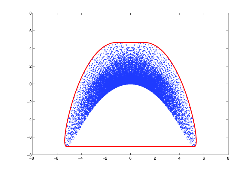
Figure 1: The dotted area is the set $V$ in Example 2.3, and the outer curve is the boundary of the convex hull $\mbox{conv}(V)$.

Example 2.3.

Consider the parametrization

$$V=\left\{\left(3x_{1}-2x_{2}-4x_{3},5x_{1}x_{2}+7x_{1}x_{3}-9x_{2}x_{3}\right):\,\|x\|_{2}\leq 1\right\}.$$

The set $V$ is drawn in the dotted area of Figure 1. By Theorem 2.1, the convex hull $\mbox{conv}(V)$ is given by the semidefinite representation

$$\left\{\begin{pmatrix}3x_{1}-2x_{2}-4x_{3}\\ 5X_{12}+7X_{13}-9X_{23}\end{pmatrix}\left|\begin{array}[]{c}\begin{bmatrix}1&x_{1}&x_{2}&x_{3}\\ x_{1}&X_{11}&X_{12}&X_{13}\\ x_{2}&X_{12}&X_{22}&X_{23}\\ x_{3}&X_{13}&X_{23}&X_{33}\end{bmatrix}\succeq 0,\\ 1-X_{11}-X_{22}-X_{33}\geq 0\end{array}\right.\right\}.$$

The boundary of the above set is the outer curve in Figure 1. One can easily see that $\mbox{conv}(V)$ is correctly given by the above semidefinite representation. ∎

3 Two homogeneous constraints

Suppose $V\subset\mathbb{R}^{m}$ is a semialgebraic set parameterized as

$$V=\{(x^{T}A_{1}x,\ldots,x^{T}A_{m}x):\,x\in T\}.$$ (3.1)

Here, every $A_{i}$ is a symmetric matrix and $T$ is defined by two homogeneous (modulo constants) inequalities/equalities $h_{j}(x)\geq 0$ or $h_{j}(x)=0$, $j=1,2$. Write

$$h_{1}(x)=x^{T}B_{1}x-c_{1},\quad h_{2}(x)=x^{T}B_{2}x-c_{2},$$

for symmetric matrices $B_{1},B_{2}$. The set $T$ is one of the four cases:

$$E(h_{1})\cap E(h_{2}),\quad S(h_{1})\cap E(h_{2}),\quad E(h_{1})\cap S(h_{2}),\quad S(h_{1})\cap S(h_{2}).$$

Note the relations:

$$x^{T}A_{i}x=A_{i}\bullet(xx^{T})\quad\,(1\leq i\leq m),\quad xx^{T}\succeq 0,$$

$$x^{T}B_{1}x=B_{1}\bullet(xx^{T}),\quad x^{T}B_{2}x=B_{2}\bullet(xx^{T}).$$

If we replace $xx^{T}$ by a symmetric matrix $X\succeq 0$, then $V$, as well as $\mbox{conv}(V)$, is contained respectively in the following projections of spectrahedra:

$$\begin{array}[]{rcl}\mathcal{H}_{e,e}&=&\{(A_{1}\bullet X,\ldots,A_{m}\bullet X):\,X\succeq 0,\,B_{1}\bullet X=c_{1},B_{2}\bullet X=c_{2}\},\\ \mathcal{H}_{i,e}&=&\{(A_{1}\bullet X,\ldots,A_{m}\bullet X):\,X\succeq 0,\,B_{1}\bullet X\geq c_{1},B_{2}\bullet X=c_{2}\},\\ \mathcal{H}_{e,i}&=&\{(A_{1}\bullet X,\ldots,A_{m}\bullet X):\,X\succeq 0,\,B_{1}\bullet X=c_{1},B_{2}\bullet X\geq c_{2}\},\\ \mathcal{H}_{i,i}&=&\{(A_{1}\bullet X,\ldots,A_{m}\bullet X):\,X\succeq 0,\,B_{1}\bullet X\geq c_{1},B_{2}\bullet X\geq c_{2}\}.\end{array}$$ (3.6)

To analyze whether they represent $\mbox{conv}(V)$ respectively, we need the following conditions for the four cases:

$$\begin{cases}C_{e,e}:\,\exists(\mu_{1},\mu_{2})\in\mathbb{R}\times\mathbb{R},\,s.t.\quad\mu_{1}B_{1}+\mu_{2}B_{2}\prec 0,\\ C_{i,e}:\,\exists(\mu_{1},\mu_{2})\in\mathbb{R}_{+}\times\mathbb{R},\,s.t.\quad\mu_{1}B_{1}+\mu_{2}B_{2}\prec 0,\\ C_{e,i}:\,\exists(\mu_{1},\mu_{2})\in\mathbb{R}\times\mathbb{R}_{+},\,s.t.\quad\mu_{1}B_{1}+\mu_{2}B_{2}\prec 0,\\ C_{i,i}:\,\exists(\mu_{1},\mu_{2})\in\mathbb{R}_{+}\times\mathbb{R}_{+},\,s.t.\quad\mu_{1}B_{1}+\mu_{2}B_{2}\prec 0.\end{cases}$$ (3.7)

Theorem 3.1.

Let $V\neq\emptyset,\mathcal{H}_{e,e},\mathcal{H}_{i,e},\mathcal{H}_{e,i},\mathcal{H}_{i,i}$ be defined as above. Then we have

$$\mbox{conv}(V)=\begin{cases}\mathcal{H}_{e,e},&\text{ if }T=E(h_{1})\cap E(h_{2})\mbox{ and }C_{e,e}\text{ holds;}\\ \mathcal{H}_{i,e},&\text{ if }T=S(h_{1})\cap E(h_{2})\mbox{ and }C_{i,e}\text{ holds;}\\ \mathcal{H}_{e,i},&\text{ if }T=E(h_{1})\cap S(h_{2})\mbox{ and }C_{e,i}\text{ holds;}\\ \mathcal{H}_{i,i},&\text{ if }T=S(h_{1})\cap S(h_{2})\mbox{ and }C_{i,i}\text{ holds.}\end{cases}$$ (3.8)

Proof.

We just prove for the case that $T=S(h_{1})\cap S(h_{2})$ and condition $C_{i,i}$ holds. The proof is similar for the other three cases. The condition $C_{i,i}$ implies that for some $\mu_{1}\geq 0,\mu_{2}\geq 0,\epsilon>0$

$$-\mu_{1}c_{1}-\mu_{2}c_{2}\geq x^{T}(-\mu_{1}B_{1}-\mu_{2}B_{2})x\geq\epsilon\|x\|_{2}^{2}.$$

So, $T$ and $\mbox{conv}(V)$ are compact. Clearly, $\mbox{conv}(V)\subseteq\mathcal{H}_{i,i}$. We need to show $\mathcal{H}_{i,i}\subseteq\mbox{conv}(V)$. Suppose otherwise it is false, then there exists a symmetric matrix $Z$ satisfying

$$(A_{1}\bullet Z,\ldots,A_{m}\bullet Z)\not\in\mbox{conv}(V),\quad B_{1}\bullet Z\geq c_{1},\quad B_{2}\bullet Z\geq c_{2},\quad Z\succeq 0.$$

Because $\mbox{conv}(V)$ is a closed convex set, by the Hahn-Banach theorem, there exists a vector $(\ell_{0},\ell_{1},\ldots,\ell_{m})\neq 0$ satisfying

$$\begin{array}[]{c}\ell_{1}x^{T}A_{1}x+\cdots+\ell_{m}x^{T}A_{m}x\geq\ell_{0}\quad\forall x\in T,\\ \ell_{1}A_{1}\bullet Z+\cdots+\ell_{m}A_{m}\bullet Z<\ell_{0}.\end{array}$$

Consider the SDP problem

$$\begin{array}[]{rl}p^{*}:=\min&\ell_{1}A_{1}\bullet X+\cdots+\ell_{m}A_{m}\bullet X\\ s.t.&X\succeq 0,\,B_{1}\bullet X\geq c_{1},\,B_{2}\bullet X\geq c_{2}.\end{array}$$ (3.9)

Its dual optimization problem is

$$\begin{array}[]{rl}\max&c_{1}\lambda_{1}+c_{2}\lambda_{2}\\ s.t.&\sum_{i}\ell_{i}A_{i}-\lambda_{1}B_{1}-\lambda_{2}B_{2}\succeq 0,\,\lambda_{1}\geq 0,\lambda_{2}\geq 0.\end{array}$$ (3.10)

The condition $C_{i,i}$ implies that the dual problem (3.10) has nonempty interior. So, the primal problem (3.9) has an optimizer. Define $\tilde{A}_{0},\tilde{B}_{1},\tilde{B}_{2}$ and a new variable $Y$ as:

$$\tilde{A}_{0}=\begin{bmatrix}\sum_{i=1}^{m}\ell_{i}A_{i}&0&0\\ 0&0&0\\ 0&0&0\end{bmatrix},\tilde{B}_{1}=\begin{bmatrix}B_{1}&0&0\\ 0&-1&0\\ 0&0&0\end{bmatrix},\tilde{B}_{2}=\begin{bmatrix}B_{2}&0&0\\ 0&0&0\\ 0&0&-1\end{bmatrix},Y=\begin{bmatrix}X&Y_{12}\\ Y_{12}^{T}&Y_{22}\end{bmatrix}.$$

They are all $(n+2)\times(n+2)$ symmetric matrices. Clearly, the primal problem (3.9) is equivalent to

$$\begin{array}[]{rl}p^{*}:=\min&\tilde{A}_{0}\bullet Y\\ s.t.&Y\succeq 0,\,\tilde{B}_{1}\bullet Y=c_{1},\,\tilde{B}_{1}\bullet Y=c_{2}.\end{array}$$ (3.11)

It must also have an optimizer. By Theorem 2.1 of Pataki [14], (3.11) has an extremal solution $U$ of rank r satisfying

$$\frac{1}{2}r(r+1)\leq 2.$$

So, we must have $r=1$ and can write $Y=vv^{T}$. Let $u=v(1:n)$. Then $u\in T$ and

$$p^{*}=\ell_{1}u^{T}A_{1}u+\cdots+\ell_{m}u^{T}A_{m}u\geq\ell_{0}.$$

However, $Z$ is also a feasible solution of (3.9), and we get the contradiction

$$p^{*}\leq\ell_{1}A_{1}\bullet Z+\cdots+\ell_{m}A_{m}\bullet Z<p^{*}.$$

Therefore, $\mathcal{H}_{i,i}\subseteq\mbox{conv}(V)$ and they must be equal. ∎

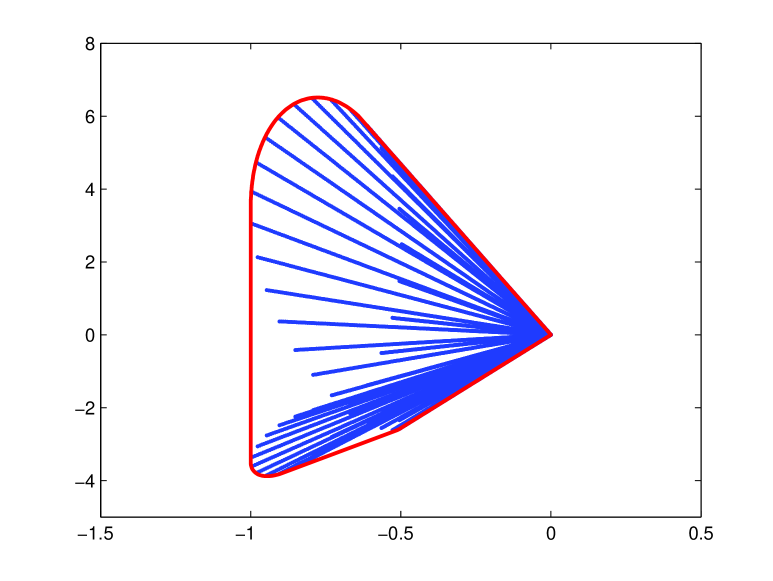
Figure 2: The dotted area is the set $V$ in Example 3.2, and the outer curve surrounds its convex hull.

Example 3.2.

Consider the parameterization

$$V=\left\{\begin{pmatrix}2x_{1}^{2}-3x_{2}^{2}-4x_{3}^{2}\\ 5x_{1}x_{2}-7x_{1}x_{3}-9x_{2}x_{3}\end{pmatrix}\left|\begin{array}[]{c}x_{1}^{2}-x_{2}^{2}-x_{3}^{2}=0,\\ 1-x^{T}x\geq 0\end{array}\right.\right\}.$$

The set $V$ is drawn in the dotted area of Figure 2. By Theorem 3.1, the convex hull $\mbox{conv}(V)$ is given by the following semidefinite representation

$$\left\{\begin{pmatrix}2X_{11}-3X_{22}-4X_{33}\\ 5X_{12}-7X_{13}-9X_{23}\end{pmatrix}\left|\begin{bmatrix}X_{11}&X_{12}&X_{13}\\ X_{12}&X_{22}&X_{23}\\ X_{13}&X_{23}&X_{33}\end{bmatrix}\succeq 0,\begin{array}[]{c}X_{11}-X_{22}-X_{33}=0,\\ 1-X_{11}-X_{22}-X_{33}\geq 0\end{array}\right.\right\}.$$

The convex region described above is surrounded by the outer curve in Figure 2, which is clearly the convex hull of the dotted area. ∎

The conditions like $C_{i,i}$ can not be removed in Theorem 3.1. We show this by a counterexample.

Example 3.3.

Consider the quadratically parameterized set

$$V=\{(x_{1}x_{2},x_{1}^{2}):\,1-x_{1}x_{2}\geq 0,1+x_{2}^{2}-x_{1}^{2}\geq 0\},$$

which is motivated by Example 4.4 of [3]. The condition $C_{i,i}$ is clearly not satisfied. The semidefinite relaxation $\mathscr{H}_{i,i}$ for $\mbox{conv}(V)$ is

$$\{(X_{12},X_{11}):\,X\succeq 0,1-X_{12}\geq 0,1+X_{22}-X_{11}\geq 0\}.$$

They are not equal, and neither are their closures. This is because $V$ is bounded above in the direction $(1,1)$, while $\mathscr{H}_{i,i}$ is unbounded (cf. [3, Example 4.4]). So, $\overline{\mbox{conv}(V)}\neq\overline{\mathscr{H}_{i,i}}$ for this example, which is due to the failure of the condition $C_{i,i}$. ∎

4 Rational parametrization

Consider the rationally parameterized set

$$U\quad=\quad\left\{\left(\frac{f_{1}(x)}{f_{0}(x)},\ldots,\frac{f_{m}(x)}{f_{0}(x)}\right):\,x\in T\right\}$$ (4.1)

with all $f_{0},\ldots,f_{m}$ being polynomials and $T$ a semialgebraic set in $\mathbb{R}^{n}$. Assume $f_{0}(x)$ is nonnegative on $T$ and every $f_{i}/f_{0}$ is well defined on $T$, i.e., the limit $\lim_{x\to z}f_{i}(x)/f_{0}(x)$ exists whenever $f_{0}$ vanishes at $z\in T$. The convex hull $\mbox{conv}(U)$ would be investigated through considering the polynomial parameterization

$$P\quad=\quad\left\{\Big{(}f_{1}^{h}(x^{h}),\ldots,f_{m}^{h}(x^{h})\Big{)}:\,f_{0}^{h}(x^{h})=1,\,x^{h}\in T^{h}\right\}.$$ (4.2)

Here $x^{h}=(x_{0},x_{1},\ldots,x_{n})$ is an augmentation of $x$ and

$$f_{i}^{h}(x^{h})\quad=\quad x_{0}^{d}f_{i}(x/x_{0})\qquad(d=\max_{i}\deg(f_{i}))$$

is a homogenization of $f_{i}(x)$, and $T^{h}$ is the homogenization of $T$ defined as

$$T^{h}=\overline{\{x^{h}:\,x_{0}>0,x/x_{0}\in T\}}.$$ (4.3)

The relation between $\mbox{conv}(V)$ and $\mbox{conv}(P)$ is given as below.

Proposition 4.1.

Suppose $f_{0}(x)$ is nonnegative on $T$ and does not vanish on a dense subset of $T$, and every $f_{i}/f_{0}$ is well defined on $T$. Then

$$\overline{\mbox{conv}(U)}\quad=\quad\overline{\mbox{conv}(P)}.$$ (4.4)

Moreover, if $T^{h}\cap\{f_{0}^{h}(x^{h})=1\}$ and $T$ are compact and $f_{0}(x)$ is positive on $T$, then

$$\mbox{conv}(U)\quad=\quad\mbox{conv}(P).$$ (4.5)

Proof.

Let $T_{1}$ be a dense subset of $T$ such that $f_{0}(x)>0$ for all $x\in T_{1}$. Clearly,

$$\overline{\mbox{conv}(U)}=\overline{\mbox{conv}\left\{\left(\frac{f_{1}^{h}(x^{h})}{f_{0}^{h}(x^{h})},\ldots,\frac{f_{m}^{h}(x^{h})}{f_{0}^{h}(x^{h})}\right):x^{h}\in T_{1}^{h}\right\}}.$$

Since every $f_{i}^{h}$ is homogeneous, we can assume that $f_{0}^{h}(x^{h})=1$. Then,

$$\overline{\mbox{conv}(U)}=\overline{\mbox{conv}\left\{\left(f_{1}^{h}(x^{h}),\ldots,f_{m}^{h}(x^{h})\right):f_{0}^{h}(x^{h})=1,\,x^{h}\in T_{1}^{h}\right\}}.$$

The density of $T_{1}$ in $T$ and the above imply (4.4).

When $T$ is compact and $f_{0}(x)$ is positive on $T$, $\mbox{conv}(U)$ is compact. The $\mbox{conv}(P)$ is also compact when $T^{h}\cap\{f_{0}^{h}(x^{h})=1\}$ is compact. Thus, (4.5) follows from (4.4). ∎

Remark: If $d=\max_{i}\deg(f_{i})$ is even and $T$ is defined by polynomials of even degrees, then we can remove the condition $x_{0}>0$ in the definition of $T^{h}$ in (4.3) and Proposition 4.1 still holds.

If every $f_{i}$ in (4.1) is quadratic, $T$ is defined by a single quadratic inequality, and $f_{0}$ is nonnegative on $T$, then a semidefinite representation for the convex hull $\mbox{conv}(U)$ or its closure can be obtained by applying Proposition 4.1 and Theorem 3.1. Suppose $T=\{x:g(x)\geq 0\}$, with $g(x)$ being quadratic. Write every $f_{i}^{h}(x^{h})=(x^{h})^{T}F_{i}\,x^{h}$ and $g^{h}(x^{h})=(x^{h})^{T}G\,x^{h}$. Then

$$\overline{\mbox{conv}(P)}\quad=\quad\overline{\mbox{conv}\left\{\Big{(}(x^{h})^{T}F_{1}\,x^{h},\ldots,(x^{h})^{T}F_{m}\,x^{h}\Big{)}:\,\begin{array}[]{c}(x^{h})^{T}F_{0}\,x^{h}=1,\\ x_{0}>0,(x^{h})^{T}G\,x^{h}\geq 0\end{array}\right\}}.$$ (4.6)

Since the forms $f_{i}^{h}$ and $g^{h}$ are all quadratic, the condition $x_{0}>0$ can be removed from the right hand side of (4.6), and we get

$$\overline{\mbox{conv}(P)}\quad=\quad\overline{\mbox{conv}\left\{\Big{(}(x^{h})^{T}F_{1}\,x^{h},\ldots,(x^{h})^{T}F_{m}\,x^{h}\Big{)}:\,\begin{array}[]{c}(x^{h})^{T}F_{0}\,x^{h}=1,\\ (x^{h})^{T}G\,x^{h}\geq 0\end{array}\right\}}.$$ (4.7)

If there are numbers $\mu_{1}\in\mathbb{R}$ and $\mu_{2}\in\mathbb{R}_{+}$ satisfying $\mu_{1}F_{0}+\mu_{2}G\prec 0$, then a semidefinite representation for $\overline{\mbox{conv}(P)}$ can be obtained by applying Theorem 3.1. The case $T=\{x:g(x)=0\}$ is defined by a single quadratic equality is similar.

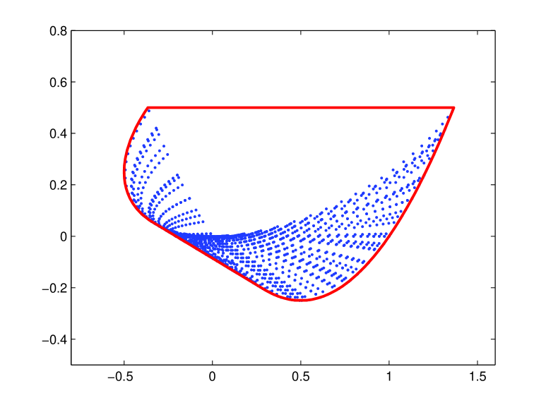
Figure 3: The dotted area is the set $U$ in Example 4.2, and the outer curve is the boundary of its convex hull.

Example 4.2.

Consider the quadratically rational parametrization:

$$U=\left\{\left(\frac{x_{1}^{2}+x_{2}^{2}+x_{3}^{2}+x_{1}+x_{2}+x_{3}}{1+x^{T}x},\frac{x_{1}x_{2}+x_{1}x_{3}+x_{2}x_{3}}{1+x^{T}x}\right):\,x_{1}^{2}+x_{2}^{2}+x_{3}^{2}\leq 1\right\}.$$

The dotted area in Figure 2 is the set $U$ above. The set $P$ in (4.2) is

$$P=\left\{\begin{pmatrix}x_{1}^{2}+x_{2}^{2}+x_{3}^{2}+x_{0}(x_{1}+x_{2}+x_{3})\\ x_{1}x_{2}+x_{1}x_{3}+x_{2}x_{3}\end{pmatrix}\left|\begin{array}[]{c}x_{0}^{2}+x_{1}^{2}+x_{2}^{2}+x_{3}^{2}=1,\\ x_{0}^{2}-x_{1}^{2}-x_{2}^{2}-x_{3}^{2}\geq 0\end{array}\right.\right\}.$$

By Theorem 3.1, the convex hull $\mbox{conv}(P)$ is given by the semidefinite representation

$$\left\{\begin{pmatrix}X_{11}+X_{22}+X_{33}+X_{01}+X_{02}+X_{03}\\ X_{12}+X_{13}+X_{23}\end{pmatrix}\left|\begin{array}[]{c}\begin{bmatrix}X_{00}&X_{01}&X_{02}&X_{03}\\ X_{01}&X_{11}&X_{12}&X_{13}\\ X_{02}&X_{12}&X_{22}&X_{23}\\ X_{03}&X_{13}&X_{23}&X_{33}\end{bmatrix}\succeq 0,\\ X_{00}+X_{11}+X_{22}+X_{33}=1,\\ X_{00}-X_{11}-X_{22}-X_{33}\geq 0\end{array}\right.\right\}.$$

The convex region described above is surrounded by the outer curve in Figure 3, which also surrounds the convex hull of the dotted area. Since $T$ is compact and the denominator $1+x^{T}x$ is strictly positive, $\mbox{conv}(U)=\mbox{conv}(P)$ by Proposition 4.1. ∎

References

• [1] C. Bayer and J. Teichmann. The proof of Tchakaloff’s Theorem. Proc. Amer. Math. Soc., 134(2006), 3035-3040.
• [2] L. Fialkow and J. Nie. Positivity of Riesz functionals and solutions of quadratic and quartic moment problems. J. Functional Analysis, Vol. 258, No. 1, pp. 328–356, 2010.
• [3] S. He, Z. Luo, J. Nie and S. Zhang. Semidefinite Relaxation Bounds for Indefinite Homogeneous Quadratic Optimization. SIAM Journal on Optimization, Vol.Β 19, No.Β 2, pp. 503–523, 2008.
• [4] J.W. Helton and J. Nie. Semidefinite representation of convex sets. Mathematical Programming, Ser.Β A, Vol. 122, No.1, pp.21–64, 2010.
• [5] J.W. Helton and J. Nie. Sufficient and necessary conditions for semidefinite representability of convex hulls and sets. SIAM Journal on Optimization, Vol. 20, No.2, pp. 759-791, 2009.
• [6] J.W. Helton and J. Nie. Structured semidefinite representation of some convex sets. Proceedings of 47th IEEE Conference on Decision and Control, pp. 4797 - 4800, Cancun, Mexico, Dec. 9-11, 2008.
• [7] W.Β Helton and V.Β Vinnikov. Linear matrix inequality representation of sets. Comm.Β Pure Appl.Β Math. 60 (2007), No. 5, pp. 654-674.
• [8] D. Henrion. Semidefinite representation of convex hulls of rational varieties. LAAS-CNRS Research Report No. 09001, January 2009.
• [9] J.Β Lasserre. Convex sets with semidefinite representation. Mathematical Programming, Vol.Β 120, No.Β 2, pp. 457–477, 2009.
• [10] J.Β Lasserre. Convexity in semi-algebraic geometry and polynomial optimization. SIAM Journal on Optimization, Vol.Β 19, No.Β 4, pp. 1995 – 2014, 2009.
• [11] J.Β Nie. First order conditions for semidefinite representations of convex sets defined by rational or singular polynomials. Mathematical Programming, to appear.
• [12] J.Β Nie. Polynomial matrix inequality and semidefinite representation. Mathematics of Operations Research, Vol.Β 36, No.Β 3, pp. 398–415, 2011.
• [13] P.Β Parrilo. Exact semidefinite representation for genus zero curves. Talk at the Banff workshop β€œPositive Polynomials and Optimization”, Banff, Canada, October 8-12, 2006.
• [14] G.Β Pataki. On the rank of extreme matrices in semidefinite programs and the multiplicity of optimal eigenvalues. Mathematics of Operations Research, 23 (2), 339–358, 1998.
• [15] M.Β Putinar. Positive polynomials on compact semi-algebraic sets, Ind. Univ. Math. J.   42 (1993) 203–206.
• [16] K.Β SchmΓΌdgen. The K-moment problem for compact semialgebraic sets. Math. Ann. 289 (1991), 203–206.