Stability of Filters for the Navier-Stokes Equation

Abstract

Data assimilation methodologies are designed to incorporate noisy observations of a physical system into an underlying model in order to infer the properties of the state of the system. Filters refer to a class of data assimilation algorithms designed to update the estimation of the state in a on-line fashion, as data is acquired sequentially. For linear problems subject to Gaussian noise filtering can be performed exactly using the Kalman filter. For nonlinear systems it can be approximated in a systematic way by particle filters. However in high dimensions these particle filtering methods can break down. Hence, for the large nonlinear systems arising in applications such as weather forecasting, various ad hoc filters are used, mostly based on making Gaussian approximations. The purpose of this work is to study the properties of these ad hoc filters, working in the context of the 2D incompressible Navier-Stokes equation. By working in this infinite dimensional setting we provide an analysis which is useful for the understanding of high dimensional filtering, and is robust to mesh-refinement. We describe theoretical results showing that, in the small observational noise limit, the filters can be tuned to perform accurately in tracking the signal itself (filter stability), provided the system is observed in a sufficiently large low dimensional space; roughly speaking this space should be large enough to contain the unstable modes of the linearized dynamics. Numerical results are given which illustrate the theory. In a simplified scenario we also derive, and study numerically, a stochastic PDE which determines filter stability in the limit of frequent observations, subject to large observational noise. The positive results herein concerning filter stability complement recent numerical studies which demonstrate that the ad hoc filters perform poorly in reproducing statistical variation about the true signal.

1 Introduction

Assimilating large data sets into mathematical models of time-evolving systems presents a major challenge in a wide range of applications. Since the data and the model are often uncertain, a natural overarching framework for the formulation of such problems is that of Bayesian statistics. However, for high dimensional models, investigation of the Bayesian posterior distribution of model state given data is not computationally feasible in on-line situations. For this reason various ad hoc filters are used. The purpose of this paper is to provide an analysis of such filters.

The paradigmatic example of data assimilation is weather forecasting: we have many complex models to predict the state of the atmosphere, currently involving on the order of ${\mathcal{O}}(10^{8})$ unknowns, but we cannot know the exact state of the system at any one time; we thus have to contend with an initial condition which is only known incompletely. This is compensated for by a large number, currently on the order of ${\mathcal{O}}(10^{6})$, partial observations of the atmosphere at subsequent times. Filters are widely used to make forecasts which combine the mathematical model of the atmosphere and the data to make predictions. Indeed the particular method of data assimilation which we study here includes, as a special case, the algorithm commonly known as 3DVAR. This method originated in weather forecasting. It was first proposed at the UK Met Office in 1986 [16], and was developed by the US National Oceanic and Atmospheric Administration (NOAA) soon thereafter; see [21]. More details of the implementation of 3DVAR by the UK Met Office can be found in [17], and by the European Centre for Medium-Range Weather Forecasts (ECMWF) in [6]. The 3DVAR algorithm is prototypical of the many more sophisticated filters which are now widely used in practice and it is thus natural to study it. The reader should be aware, however, that the development of new filters is a very active area and that the analysis here constitutes an initial step towards the analyses required for these more recently developed algorithms. For insight into some of these more sophisticated filters see [27, 9, 28, 11, 19] and the references therein.

Filtering can be performed exactly for linear systems subject to Gaussian noise: the Kalman filter [12]. For nonlinear or non-Gaussian scenarios the particle filter [8] may be used and provably approximates the desired probability distribution as the number of particles is increased [1]. However in practice this method performs poorly in high dimensional systems [23]. Whilst there is considerable research activity aimed at overcoming this degeneration [29, 3], the methodology cannot yet be viewed as a provably accurate tool within the context of the high dimensional problems arising in geophysical data assimilation. In order to circumvent problems associated with the representation of high dimensional probability distributions some form of ad hoc Gaussian approximation is typically used to create practical filters, and the 3DVAR method which we analyze here is perhaps the simplest example of this.

In the paper [15] a wide range of Gaussian approximate filters, including 3DVAR, are evaluated by comparing the distributions they produce with a highly accurate (and impractical in realistic online scenarios) MCMC simulation of the desired distributions. The conclusion of that work is that the Gaussian approximate filters perform well in tracking the mean of the desired distribution, but poorly in terms of statistical variability about the mean. In this paper we provide a theoretical analysis of the ability of the filters to estimate the mean state accurately. Although filtering is widely used in practice, much of the analysis of it, in the context of fluid mechanics, works with finite-dimensional dynamical models. Our aim is to work directly with a PDE model relevant in fluid mechanics, the Navier-Stokes equation, and thereby confront the high-dimensional nature of the problem head-on. Study of the stability of filters for data assimilation has been a developing research area over the last few years and the paper [2] contains a finite dimensional theoretical result, numerical experiments in a variety of finite and (discretized) infinite dimensional systems not covered by the theory, and references to relevant applied literature. Our analysis will build in a concrete fashion on the approach in [20] and [13] which were amongst the first to study data assimilation directly through PDE analysis, using ideas from the theory of determining modes in infinite dimensional dynamical systems. However, in contrast to those papers, we will allow for noisy observations in our analysis. Nonetheless the estimates in [13] form an important component of our analysis.

The presentation will be organized as follows: in Section 2 we introduce the Navier-Stokes equation as the forward model; in Section 3 we formulate data assimilation as a Bayesian inverse problem and show how approximate Gaussian filters can be derived, leading to 3DVAR and generalizations; in Section 4 we introduce notions of stability and prove the Main Theorems 4.3 and 4.7 concerning filter stability for sufficiently small observational noise; section 4 also contains derivation of the stochastic PDE (SPDE) and deterministic PDE which may be used to study filter stability for 3DVAR when data is aquired frequently in time and the observational noise is large; in Section 5 we present numerical results which corroborate the analysis; and finally, in Section 6 we present conclusions. The mathematical tools required to follow the arguments in this paper comprise basic ideas from probability on Hilbert space, properties of the Navier-Stokes equation, analysis of nonautonomous/random dynamical systems, and properties of stochastic PDEs. Together these tools facilitate an analysis which allows mathematical study of filtering and, we believe, can be built upon to study other problems arising in the filtering of complex systems.

2 Forward Model: Navier-Stokes equation

In this section we establish a notation for, and describe the properties of, the Navier-Stokes equation. This is the forward model which underlies the inverse problem which we study in this paper. We consider the 2D Navier-Stokes equation on the torus $\mathbb{T}^{2}:=[0,L)\times[0,L)$ with periodic boundary conditions:

$$\begin{array}[]{cccc}\partial_{t}u-\nu\Delta u+u\cdot\nabla u+\nabla p&=&f&{\rm for~{}all~{}}(x,t)\in\mathbb{T}^{2}\times(0,\infty),\\ \nabla\cdot u&=&0&{\rm for~{}all~{}}(x,t)\in\mathbb{T}^{2}\times(0,\infty),\\ u(x,0)&=&u_{0}(x)&{\rm for~{}all~{}}x\in\mathbb{T}^{2}.\end{array}$$

Here $u\colon\mathbb{T}^{2}\times(0,\infty)\to\mathbb{R}^{2}$ is a time-dependent vector field representing the velocity, $p\colon\mathbb{T}^{2}\times(0,\infty)\to\mathbb{R}$ is a time-dependent scalar field representing the pressure, $f\colon\mathbb{T}^{2}\to\mathbb{R}^{2}$ is a vector field representing the forcing (which we assume to be time-independent for simplicity), and $\nu$ is the viscosity. In numerical simulations (see section 5), we typically represent the solution via the vorticity $w$ and stream function $\zeta$; these are related through $u=\nabla^{\perp}\zeta$ and $w=\nabla^{\perp}\cdot u$, where $\nabla^{\perp}=(\partial_{2},-\partial_{1})^{\mathrm{T}}$. We define

$${\mathcal{H}}:=\left\{L{\rm{-periodic\,trigonometric\,polynomials\,}}u:[0,L)^{2}\to{\mathbb{R}}^{2}\,\Bigl{|}\,\nabla\cdot u=0,\,\int_{\mathbb{T}^{2}}u(x)\,\mathrm{d}x=0\right\}$$

and $H$ as the closure of ${\mathcal{H}}$ with respect to the $(L^{2}(\mathbb{T}^{2}))^{2}$ norm. We define $P:(L^{2}(\mathbb{T}^{2}))^{2}\to H$ to be the Leray-Helmholtz orthogonal projector.

Given $k=(k_{1},k_{2})^{\mathrm{T}}$, define $k^{\perp}:=(k_{2},-k_{1})^{\mathrm{T}}$. Then an orthonormal basis for $H$ is given by $\psi_{k}\colon\mathbb{R}^{2}\to\mathbb{R}^{2}$, where

$$\psi_{k}(x):=\frac{k^{\perp}}{|k|}\exp\Bigl{(}\frac{2\pi ik\cdot x}{L}\Bigr{)}$$

for $k\in\mathbb{Z}^{2}\setminus\{0\}$. Thus for $u\in H$ we may write

$$u=\sum_{k\in\mathbb{Z}^{2}\setminus\{0\}}u_{k}(t)\psi_{k}(x)$$

where, since $u$ is a real-valued function, we have the reality constraint $u_{-k}=-\overline{u_{k}}.$ We then define the projection operators $P_{\lambda}:H\to H$ and $Q_{\lambda}:H\to H$ by

$$P_{\lambda}u=\sum_{|2\pi k|^{2}<\lambda L^{2}}u_{k}(t)\psi_{k}(x),\quad Q_{\lambda}=I-P_{\lambda}.$$

We let $W_{\lambda}=P_{\lambda}H$ and $W_{\lambda}^{c}=Q_{\lambda}H.$

Using the Fourier decomposition of $u$, we define the fractional Sobolev spaces

$$H^{s}:=\left\{u\in H:\sum_{k\in\mathbb{Z}^{2}\setminus\{0\}}(4\pi^{2}|k|^{2})^{s}|u_{k}|^{2}<\infty\right\}$$ (2)

with the norm $\|u\|_{s}:=\bigl{(}\sum_{k}(4\pi^{2}|k|^{2})^{s}|u_{k}|^{2}\bigr{)}^{1/2}$, where $s\in\mathbb{R}$. We use the abbreviated notation $\|u\|$ for the norm on $H^{1}$, and $|\cdot|$ for the norm on $H=H^{0}$.

Applyng the projection $P$ to the Navier-Stokes equation we may write it as an ODE (ordimary differential equation) in $H$; see [4, 25, 22] for details. This ODE takes the form

$$\frac{\mathrm{d}u}{\mathrm{d}t}+\nu Au+\mathcal{B}(u,u)=f,\quad u(0)=u_{0}.$$ (3)

Here, $A=-P\Delta$ is the Stokes operator, the term $\mathcal{B}(u,u)=P(u\cdot\nabla u)$ is the bilinear form found by projecting the nonlinear term $u\cdot\nabla u$ into $H$ and finally, with abuse of notation, $f$ is the original forcing, projected into $H$. We note that $A$ is diagonalized in the basis comprised of the $\{\psi_{k}\}_{k\in{\mathbb{Z}}^{2}\backslash\{0\}}$, on $H$, and the smallest eigenvalue of $A$ is $\lambda_{1}=4\pi^{2}/L^{2}.$ The following proposition is a classical result which implies the existence of a dissipative semigroup for the ODE (3). See Theorems 9.5 and 12.5 in [22] for a concise overview and [25, 26] for further details.

Proposition 2.1.

Assume that $u_{0}\in H^{1}$ and $f\in H$. Then (3) has a unique strong solution on $t\in[0,T]$ for any $T>0:$

$$u\in L^{\infty}\bigl{(}(0,T);H^{1}\bigr{)}\cap L^{2}\bigl{(}(0,T);D(A)\bigr{)},\quad\frac{du}{dt}\in L^{2}\bigl{(}(0,T);H\bigr{)}.$$

Furthermore the equation has a global attractor $\mathcal{A}$ and there is $K>0$ such that, if $u_{0}\in\mathcal{A}$, then $\sup_{t\geq 0}\|u(t)\|^{2}\leq K.$

We let $\{\Psi(\cdot,t):H^{1}\to H^{1}\}_{t\geq 0}$ denote the semigroup of solution operators for the equation (3) through $t$ time units. We note that by working with weak solutions, $\Psi(\cdot,t)$ can be extended to act on larger spaces $H^{s}$, with $s\in[0,1)$, under the same assumption on $f$; see Theorem 9.4 in [22]. We will, on occasion, use this extension of $\Psi(\cdot,t)$ to act on larger spaces. In particular we use it in the following proposition which follows from Lemmas 5.3 and 5.5 in [5]. This proposition is key to enabling us to show that the Bayesian inverse problem, which underlies the filtering problem of interest, is well-posed.

Proposition 2.2.

Let $s\in(0,1]$ and $t_{0}>0.$ Then, for all $t>t_{0}$, and $u,v\in H$,

$$\begin{array}[]{ll}\|\Psi(u,t)\|_{s}^{2}&\leq t_{0}^{-s}C\bigl{(}|f|^{2}+|u|^{2})\\ \|\Psi(u,t)-\Psi(v,t)\|_{s}^{2}&\leq t_{0}^{-s}C\bigl{(}|u|,|u-v|,|f|\bigr{)}|u-v|^{2}.\end{array}$$

The key properties of the Navier-Stokes equation that drive our analysis of the filters are summarized in the following proposition, taken from the paper [13]. To this end, define $\Psi(\cdot)=\Psi(\cdot,h)$ for some fixed $h>0.$ Note that the statement here is closely related to the squeezing property [22] of the Navier-Stokes equation, a property employed in a wide range of applied contexts.

Proposition 2.3.

Let $u\in\mathcal{A}$ and $v\in H^{1}$. There is $\beta=\beta(|f|,L,\nu)>0$ such that

$$\|\Psi(u)-\Psi(v)\|^{2}\leq\exp(\beta h)\|u-v\|^{2}.$$ (5)

Now let $\|u-v\|\leq R$ and assume that

$$\lambda>\lambda^{\star}:=\frac{9c^{8/3}}{\lambda_{1}^{\frac{1}{3}}}\Bigl{(}\frac{2K^{\frac{1}{2}}+R^{\frac{1}{2}}}{\nu}\Bigr{)}^{8/3}$$

where $c$ is a dimensionless positive constant. Then there exists $t^{*}=t^{*}(|f|,L,\nu,\lambda,R)$ with the property that, for all $h\in(0,t^{*}],$ there is $\gamma\in(0,1)$ such that

$$\|Q_{\lambda}\bigl{(}\Psi(u)-\Psi(v)\bigr{)}\|^{2}\leq\gamma^{2}\|u-v\|^{2}.$$ (6)

Proof.

The first statement is simply Theorem 3.8 from [13]. The second statement follows from the proof of Theorem 3.9 in the same paper, modified at the end to reflect the fact that, in our setting, $P_{\lambda}\delta(0)\neq 0.$ Note also that the constant $\lambda$ appearing on the right hand side of the lower bound for $\lambda$ in the statement of Theorem 3.9 in [13] should be $\lambda_{1}$ (as the proof that follows in [13] shows) and that use of definition of $K$ (see Theorem 3.6 of that paper) allows rewrite in terms of $K$ – indeed the proof in that paper is expressed in terms of $K$. ∎

3 Inverse Problem: Filtering

In this section we describe the basic problem of filtering the Navier Stokes equation (3): estimating properties of the state of the system sequentially from partial, noisy, sequential observations of the state. We first set up the inverse problem of interest, in subsection 3.1. Then, in subsection 3.2, we describe the full statistical filtering distribution. We describe the approximate Gaussian filters, which are the focus of the remainder of the paper, in subsection 3.3; in subsection 3.4 we make a brief remark concerning the extension to completely observed systems. We conclude with subsection 3.5 which introduces 3DVAR as an example of the approximate Gaussian filter.

3.1 Setup

Throughout the following we write $\mathbb{N}$ for the natural numbers $\{1,2,3,\dots\}$, and $\mathbb{Z}^{+}:=\mathbb{N}\cup\{0\}$ for the non-negative integers $\{0,1,2,3,\dots\}$. Recall that we have defined $\Psi(\cdot)=\Psi(\cdot,h)$ for some fixed $h>0.$ Our interest is in determining $u$ from noisy observations of $P_{\lambda}u$. We let $X$ denote $H^{s}$ for any $s\geq 1$ and define $\{u_{j}\}_{j\in\mathbb{Z}^{+}}$, $u_{j}\in X$ by

$$u_{j+1}:=\Psi(u_{j}).$$ (7)

Thus $u_{j}=u(jh)$ where $u$ solves (3). We now let $\{{\xi}_{j}\}_{j\in\mathbb{N}}$ be a noise sequence in $W_{\lambda}$ which perturbs the sequence $\{P_{\lambda}u_{j}\}_{j\in\mathbb{N}}$ to generate the observation sequence $\{y_{j}\}_{j\in\mathbb{N}}$ in $W_{\lambda}$ given by

$$y_{j+1}:=P_{\lambda}u_{j+1}+{\xi}_{j+1},\quad j\in\mathbb{Z}^{+}.$$ (8)

We let $Y_{j}=\{y_{i}\}_{i=1}^{j}$, the accumulated data up to time $t=jh.$ We assume that $u_{0}$ is not known exactly. The goal of filtering is to determine information about the state $u_{j}$ from the data $Y_{j}.$ Mathematically, it is natural to formulate this as a Bayesian inverse problem, and this viewpoint is described in subsection 3.2.

3.2 Filtering Distribution

In the statistical formulation of the filtering problem we assume that $(u_{0},Y_{j})$ is a random variable on $(X,W_{\lambda}^{j})$, defined by specifying the distributions of $u_{0}$ (the prior) and $=\{\xi_{i}\}_{1\leq i\leq j}$ (the observational noises) which is assumed to be an i.i.d. sequence. The aim is to find the conditional probability distribution on $u_{0}$ given a single realization of $Y_{j}$, and we denote this conditional distribution by $\mathbb{P}(u_{0}|Y_{j}).$ The filtering distribution, namely the probability distribution on $u_{j}$ given $Y_{j}$, denoted by $\mathbb{P}_{j}(u_{j}|Y_{j})$, is then found as the image of $\mathbb{P}(u_{0}|Y_{j})$ under the map $\Psi(\cdot;jh).$ In finite dimensions carrying out this program is a straightforward application of Bayes’ theorem. Here we show how similar ideas may be applied in the infinite dimensional setting. We make the following assumption.

Assumption 3.1.

The prior distribution on $u_{0}$ is a Gaussian $\mathbb{P}_{0}(u_{0})=N({\widehat{m}}_{0},{\widehat{\mathcal{C}}}_{0})$, with the property that $\mathbb{P}_{0}(H)=1.$ The observational noise sequence $\{\xi_{j}\}_{j\in\mathbb{N}}$ is an i.i.d sequence in $W_{\lambda}$, independent of $u_{0}$, with $\xi_{1}$ distributed according to a Gaussian measure $N(0,\Gamma)$ on $W_{\lambda}$, with $\Gamma$ strictly positive on $W_{\lambda}$.

Under this assumption the Bayesian inverse problem has a well-defined solution, and exhibits well-posedness with respect to the data, in the Hellinger metric (see [5] for a definition).

Theorem 3.2.

Let Assumption 3.1 hold. The measure $\mathbb{P}(u_{0}|Y_{j})$ is absolutely continuous with respect to $\mathbb{P}_{0}(u_{0})$ with Radon-Nikodym derivative given by

$$\frac{d\mathbb{P}}{d\mathbb{P}_{0}}(u_{0}|Y_{j})\propto\exp\Bigl{(}-\Phi^{(j)}(u_{0})\Bigr{)}.$$ (9)

Here

$$\Phi^{(j)}(w)=\frac{1}{2}\sum_{i=1}^{j}\Bigl{|}\Gamma^{-\frac{1}{2}}\Bigl{(}y_{i}-P_{\lambda}\Psi(w;ih)\Bigr{)}\Bigr{|}^{2}.$$ (10)

Furthermore, $\mathbb{P}(u_{0}|Y_{j})$ is Lipschitz in $Y_{j}$ with respect to the Hellinger metric.

Proof.

Note that $W_{\lambda}$ is a finite dimensional space. The result can thus be deduced from Corollary 2.2 and Theorem 2.5 in [5]. To apply Corollary 2.2 it suffices to show that $\Psi(\cdot;ih)\colon H\to H$ is continuous for any $i\in{\mathbb{Z}}$ since then $P_{\lambda}\Psi(\cdot;ih)\colon H\to W_{\lambda}$ is continuous; the required continuity follows from the second item of Proposition 2.2. To apply Theorem 2.5 it suffices to show that $\Psi(\cdot;ih)\colon H\to H$ is polynomially bounded, since then $\Phi^{(j)}\colon H\to\mathbb{R}^{+}$, and its Lipschitz constant with respect to data $Y_{j}$, are both polynomially bounded. This polynomial boundedness of $\Psi$ follows from the first item of Proposition 2.2. ∎

The measure $\mathbb{P}_{j}(u_{j}|Y_{j})$ is then defined by the push-forward under the semigroup $\Psi(\cdot;jh)$ and Proposition 2.2 gives the following corollary:

Corollary 3.3.

Let Assumption 3.1 hold. Then the sequence of measures $\{\mathbb{P}_{j}(u_{j}|Y_{j})\}_{j\geq 0}$ is well-defined by

$$\mathbb{P}_{j}(\cdot|Y_{j})=\Psi(\cdot;jh)\star\mathbb{P}(\cdot|Y_{j})$$

where $\mathbb{P}(\cdot|Y_{j})$ is given in Theorem 3.2. Furthermore, for $v\sim\mathbb{P}_{j}(\cdot|Y_{j})$, $v\in H^{1}$ with probability one.

3.3 Approximate Gaussian Filters; Partial Observations

The measures $\mathbb{P}(u_{0}|Y_{j})$ and $\mathbb{P}_{j}(u_{j}|Y_{j})$ determined in Theorem 3.2 and Corollary 3.3 are, in practice, very hard to compute by statistical sampling methods. Sequential Monte Carlo methods (SMC) can in principle be applied to determine the $\mathbb{P}_{j}(u_{j}|Y_{j})$, but new ideas are required to extend them to problems in high dimensions [23]. The measure $\mathbb{P}(u_{0}|Y_{j})$ has the advantage of being specified via density with respect to a Gaussian and it is shown in [15] that, building on this fact, Markov chain-Monte Carlo (MCMC) methods can be used successfully to approximate $\mathbb{P}(u_{0}|Y_{j})$ when the dynamics of (3) are mildly turbulent; but these methods are very expensive indeed, and do not exploit the sequential nature of the problem as $j$ is incremented. Sequential methods are attractive for online applications and for this reason various ad hoc approximation methods are used which lead to tractable sequential algorithms. A commonly made approximation is to impose a Gaussian structure on the filtering distributions so that

$$\mathbb{P}_{j}(u_{j}|Y_{j})\approx N(\widehat{m}_{j},\widehat{\mathcal{C}}_{j}).$$ (11)

The key question in designing an approximate Gaussian filter, then, is to find an update rule of the form

$$(\widehat{m}_{j},\widehat{\mathcal{C}}_{j})\mapsto(\widehat{m}_{j+1},\widehat{\mathcal{C}}_{j+1}).$$ (12)

Because of the linear form of the observations in (8), together with the fact that the noise is mean zero-Gaussian, this update rule is determined directly if we use the Gaussian assumption that the distribution of $u_{j+1}$ given $Y_{j}$ is Gaussian:

$$u_{j+1}|Y_{j}\sim N(m_{j+1},\mathcal{C}_{j+1}).$$ (13)

In general, even if the approximation (11) is a good one, there is no reason to expect (13) to be a good approximation since the distribution on $u_{j+1}|Y_{j}$ is the pushforward of $\mathbb{P}_{j}(u_{j}|Y_{j})$, assumed Gaussian, under the nonlinear map $\Psi(\cdot;h)$ and in general only linear transformations preserve Gaussianity. However, in this paper, we will simply impose the approximation (13) with

$$m_{j+1}=\Psi(\widehat{m}_{j};h)$$ (14)

and with $\mathcal{C}_{j+1}$ specified exogenously. This then defines the map (12), as we now show.

Assumption 3.4.

Assume that $u_{j+1}|Y_{j}$ is specified by (13) for $m_{j+1}$ given by (14) and covariance operator $\mathcal{C}_{j+1}$ on $H$ which is strictly positive on $W_{\lambda}$ and which commutes with $A$. Assume further that $y_{j+1}|u_{j+1}$ is given by (8) where the random variable $\xi_{j+1}$ is a mean zero Gaussian in $W_{\lambda}$ with covariance $\Gamma$ a strictly positive operator on $W_{\lambda}$ which commutes with $A$.

Note that the Gaussian $N(m_{j+1},\mathcal{C}_{j+1})$ factors as the product of two independent Gaussians on $W_{\lambda}$ and $W_{\lambda}^{c}$, because $\mathcal{C}_{j+1}$ commutes with $A$; to avoid proliferation of notation, we also denote by $\mathcal{C}_{j+1}$ the covariance operator restricted to $W_{\lambda}$ and $W_{\lambda}^{c}$. The factoring as independent products is inherited by the resulting Gaussian approximation for $u_{j+1}|Y_{j+1}$ as the following charactertization shows.

Theorem 3.5.

Let Assumption 2 hold. Then $u_{j+1}|Y_{j+1}$ is Gaussian on $H$ and factors as the product of two indepenent Gaussians on $W_{\lambda}$ and $W_{\lambda}^{c}$. Denoting the mean and covariance of both of these independent Gaussians by $\widehat{m}_{j+1}$ and $\widehat{C}_{j+1}$ respectively we have

$$\begin{array}[]{ccccc}\widehat{C}_{j+1}&=\mathcal{C}_{j+1},{}{}&\quad\widehat{m}_{j+1}&=Q_{\lambda}\Psi(\widehat{m}_{j}),{}{}{}&\quad{\rm{on}}\,\,W_{\lambda}^{c}\\ {\widehat{\mathcal{C}}}_{j+1}^{-1}&=\mathcal{C}_{j+1}^{-1}+\Gamma^{-1},&\quad{\widehat{\mathcal{C}}}_{j+1}^{-1}\widehat{m}_{j+1}&=\mathcal{C}_{j+1}^{-1}P_{\lambda}\Psi(\widehat{m}_{j})+\Gamma^{-1}y_{j+1},&\quad{\rm{on}}\,\,W_{\lambda}.\end{array}$$

Proof.

For economy of notation, let $v$ denote the random variable $u_{j+1}|Y_{j}$ and $y$ the random variable $y_{j+1}$. Under the stated assumptions, $(v,y)$ is a jointly Gaussian random variable and we are interested in finding the conditional distribution of $v|y$ (which is the desired distribution of $u_{j+1}|Y_{j+1}.$) Let $\nu(dv,dy)$ denote the Gaussian distribution of $(v,y)$ and let $\nu_{0}(dv,dy)$ denote the Gaussian distribution specified as the independent product of the Gaussian measures $\mu_{0}=N(m_{j+1},\mathcal{C}_{j+1})$ and $N(0,\Gamma).$ From the properties of finite dimensional Gaussians it is immediate that $\nu$ has density with respect to $\nu_{0}$ and that

$$\frac{d\nu}{d\nu_{0}}(v,y)=\exp\Bigl{(}-\frac{1}{2}\bigl{|}\Gamma^{-\frac{1}{2}}(y-P_{\lambda}v)\bigr{|}^{2}+\frac{1}{2}\bigl{|}\Gamma^{-\frac{1}{2}}y\bigr{|}^{2}\Bigr{)}.$$

If $\mu$ is the desired conditional distribution on $v|y$, then Lemma 2.3 in [5] gives

$$\frac{d\mu}{d\mu_{0}}(v)\propto\exp\Bigl{(}-\frac{1}{2}\bigl{|}\Gamma^{-\frac{1}{2}}(y-P_{\lambda}v)\bigr{|}^{2}\Bigr{)}$$

with constant of proportionality depending only on $y$. Note that $\mu_{0}$ factors in the desired fashion on $W_{\lambda}$ and $W_{\lambda}^{c}$, and that the change of measure depends only on $P_{\lambda}v$; hence $\mu$ factors in the same fashion. Furthermore, since the change of meausure depends only on (the finite dimensional) $P_{\lambda}v\in W_{\lambda}$, completing the square gives the expression for the measure in $W_{\lambda}$, and in $W_{\lambda}^{c}$ we have $\mu=\mu_{0}$. This completes the proof. ∎

It is demonstrated numerically in [15] that Gaussian approximations of the filtering distribution such as the one characterized in the preceding theorem are, in general, not good approximations. More precisely, they fail to accurately capture covariance information. However, the same numerical experiments reveal that the methodology can perform well in replicating the mean, if parameters are chosen correctly, even if it is initially in error. Indeed this accurate tracking of the mean is often achieved by means of variance inflation – increasing the model uncertainty, here captured in the exogenously imposed $\mathcal{C}_{j}$, in comparison with the data uncertainty, here captured in the $\Gamma$. The purpose of the remainder of the paper is to explain, and illustrate, this phenomenon by means of analysis and numerical experiments. To this end we introduce a compact notation for the mean update $\widehat{m}_{j}\mapsto\widehat{m}_{j+1}.$

We define an operator $B_{j}\colon W_{\lambda}\times W_{\lambda}^{c}\mapsto W_{\lambda}\times W_{\lambda}^{c}$ by

$$B_{j}=\left(\begin{array}[]{cc}{\widehat{\mathcal{C}}}_{j+1}\mathcal{C}_{j+1}^{-1}&0\\ 0&{\widehat{\mathcal{C}}}_{j+1}\mathcal{C}_{j+1}^{-1}\end{array}\right)$$ (18)

where ${\widehat{\mathcal{C}}}_{j+1}$ and $\mathcal{C}_{j+1}$ denote the covariances in $W_{\lambda}$ (resp. $W_{\lambda}^{c}$) in the top left (resp. bottom right) entries of $B_{j}$. We also extend $y_{j+1}$ from an element of $W_{\lambda}$ to an element of $H$ in the canonical fashion, by defining it to be zero in $W_{\lambda}^{c}$. Then Theorem 3.5 yields the key equation

$$\widehat{m}_{j+1}=B_{j}\Psi(\widehat{m}_{j};h)+(I-B_{j})y_{j+1},$$ (19)

which demonstrates that the estimate of the mean at time $j+1$ is found as an operator-convex combination of the true dynamics applied to the estimate of the mean at time $j$, and the data at time $j+1$. Note that, in the case of a linear dynamical system where $\Psi(\cdot;h)$ is a linear map, the matrix $I-B_{j}$ is the Kalman gain matrix [12].

3.4 Approximate Gaussian Filters; Complete Observations

We will also study the situation where complete observations are made, obtained by taking $\lambda\to\infty$ in the preceding analyses. The observations are given by

$$y_{j}:=u_{j}+{\xi}_{j},\quad j\in\mathbb{Z}^{+}$$ (20)

where now $y_{j},\xi_{j}\in H$ and the i.i.d. mean zero Gaussian sequence $\{\xi_{j}\}_{j\in\mathbb{N}}$ is defined by a covariance operator $\Gamma$ on $H$.

It is possible to characterize the full filtering distribution in this setting, but rather technical to do so; the example of the inverse problem for the heat equation in [24] illustrates the technicalities involved. Because of this we concentrate on studying only the equation for the mean update in the approximate Gaussian filter. This takes the form (19) where, on the whole of $H$, we have

$$B_{j}={\widehat{\mathcal{C}}}_{j+1}\mathcal{C}_{j+1}^{-1},\quad{\widehat{\mathcal{C}}}_{j+1}^{-1}=\mathcal{C}_{j+1}^{-1}+\Gamma^{-1}.$$ (21)

3.5 Example of an Approximate Gaussian Filter: 3DVAR

The algorithm described in the previous section yields the well-known 3DVAR method, discussed in the introduction, when $\mathcal{C}_{j}\equiv\mathcal{C}$ for some fixed operator $\mathcal{C}$. To impose commutativity with $A$, we assume that the operators $\Gamma$ and $\mathcal{C}$ are both fractional powers of the Stokes operator $A$, in $W_{\lambda}$ and $H$ respectively. Note that fixing $\mathcal{C}_{j}\equiv\mathcal{C}$ implies that ${\widehat{\mathcal{C}}}_{j}\equiv{\widehat{\mathcal{C}}}$ where

$$\begin{array}[]{cc}{\widehat{\mathcal{C}}}^{-1}&=\mathcal{C}^{-1}+\Gamma^{-1},\quad{\rm in}\,\,W_{\lambda}\\ {\widehat{\mathcal{C}}}^{-1}&=\mathcal{C}^{-1},\quad\quad\quad~{}~{}{\rm in}\,\,W_{\lambda}^{c}.\end{array}$$

We choose $A_{0}=\ell A$ and set $\mathcal{C}=\delta^{2}A_{0}^{-2\zeta}$ in $H$ and $\Gamma=\sigma^{2}A_{0}^{-2\beta}$ in $W_{\lambda}.$ Substituting into the update formula (19) for $\widehat{m}_{j}$ and defining $\eta=\sigma/\delta,$ $\alpha=\zeta-\beta$, $B_{0}({\eta})=(I+\eta^{2}A_{0}^{2\alpha})^{-1}\eta^{2}A_{0}^{2\alpha}$ in $W_{\lambda}$ then (18) gives a constant matrix

$$B=\left(\begin{array}[]{cc}B_{0}({\eta})&0\\ 0&I\end{array}\right).$$ (25)

Using this we obtain the mean update formula

$$\widehat{m}_{j+1}=B\Psi(\widehat{m}_{j})+(I-B)y_{j+1}.$$ (26)

Notice that for $\mathcal{C},\Gamma$ given as above, the algorithm depends only on the three parameters $\lambda,\alpha$ and $\eta$, once the constant of proportionality $\ell$ in $A_{0}$ is set. The parameter $\lambda$ measures the size of the space in which observations are made; for fixed wavevector $k$, the parameter $\eta$ is a measure of the scale of the uncertainty in observations to uncertainty in the model; and the sign of the parameter $\alpha$ determines whether, for fixed $\eta$ and asymptotically for large wavevectors, the model is trusted more ($\alpha>0$) or less ($\alpha<0$) than the data.

In the case $\lambda=\infty$, the case of complete observations where the whole velocity field is noisily observed, we again obtain (26), with $B=B_{0}({\eta})=(I+\eta^{2}A_{0}^{2\alpha})^{-1}\eta^{2}A_{0}^{2\alpha}$ in $H$.The roles of $\eta$ and $\alpha$ are the same as in the finite $\lambda$ (partial observations) case.

The discussion concerning parametric dependence with respect to varying $\eta$ shows that, for the example of 3DVAR introduced here, and for both $\lambda$ finite and infinite, variance inflation can be achieved by decreasing the parameter $\eta.$ We will show that variance inflation does indeed improve the ability of the filter to track the signal.

4 Stability

In this section we develop conditions under which it is possible to prove stability of the nonautonomous dynamical system defined by the mean update equation (19). By stability we here mean that, when the noise perturbing the observations is ${\mathcal{O}}(\epsilon)$, the mean update will converge to an ${\mathcal{O}}(\epsilon)$ neighbourhood of the true signal, even if initially it is an ${\mathcal{O}}(1)$ distance from the true signal. In subsection 4.1 we study the case of partial observations; subsection 4.2 contains the (easier) result for the case of complete observations. The third subsection 4.3 shows how our results can be applied to the specific instance of the 3DVAR algorithm introduced in subsection 3.5, for any $\alpha\in{\mathbb{R}}$, provided $\eta$, which is a measure of uncertainty in the data to uncertainty in the model, is sufficiently small: this, then, is a result concerning variance inflation. In the final subsection 4.4 we also consider 3DVAR in the case of frequent observations and large $\eta$, deriving an SPDE and a PDE, both of which may be used to study filter stability.

For simplicity, we will assume a “truth” which is on the global attractor, as in [13]. This is not necessary, but streamlines the presentation as it gives an automatic uniform in time bound in $H^{1}$. Recall that $\|\cdot\|$ denotes the norm in $H^{1}$, and $|\cdot|$ the norm in $H$; similarly we lift $\|\cdot\|$ to denote the induced operator norm $H^{1}\to H^{1}$.

4.1 Main Result: Partial Observations

In this case we will see that it is crucial that the observation space $W_{\lambda}$ is sufficiently large, i.e. that a sufficiently large number of modes are observed. This, combined with the contractivity in the high modes encapsulated in Proposition 2.3 from [13], can be used to ensure stability if combined with variance inflation.

We study filters of the form given in (19) and make the following assumption on the observations $\{y_{j}\}.$ We note that this assumption is incompatible with the Gaussian assumptions used to derive the filter and we return to this point when describing numerical results in section 5.

Assumption 4.1.

Consider a sequence $u_{j}=u(jh)$ where $u(t)$ is a solution of (3) lying on the global attractor $\mathcal{A}$. Then, for some $\lambda\in(\lambda_{1},\infty)$,

$$y_{j}=P_{\lambda}u_{j}+\xi_{j}$$

for some sequence $\xi_{j}$ satisfying $\sup_{j\geq 1}\|\xi_{j}\|\leq\epsilon.$

We make the following assumption about the family $\{B_{j}\}$, and assumed dependence on a parameter $\eta\in{\mathbb{R}}^{+}.$ Recall that the inverse of $\eta$ quantifies the amount of variance inflation.

Assumption 4.2.

The family of positive operators $\{B_{j}(\eta)\colon H^{1}\to H^{1}\}_{j\geq 1}$ commute with $A$, satisfy $\sup_{j\geq 1}\|B_{j}(\eta)\|\leq 1$, and $\sup_{j\geq 1}\|I-B_{j}(\eta)\|\leq b$ for some $b\in{\mathbb{R}}^{+},$ uniformly with respect to $\eta$. Furthermore, $\bigl{(}I-B_{j}(\eta)\bigr{)}Q_{\lambda}\equiv 0$ and there is, for all $\lambda>\lambda_{1}$, constant $c=c(\lambda)>0$ such that $\sup_{j\geq 1}\|P_{\lambda}B_{j}(\eta)\|\leq c\eta^{2}.$

We now study the asymptotic behaviour of the filter under these assumptions.

Theorem 4.3.

Let Assumptions 4.1 and 4.2 hold, choose any $\widehat{m}_{0}\in\mathbb{B}_{H^{1}}\bigl{(}u(0),r\bigr{)}$ and let $(\lambda^{*},t^{*})$ be as given in Proposition 2.3. Assume that $\lambda>\lambda^{*}$. Then for any $h\in(0,t^{*}]$ there is $\eta$ sufficiently small so that the sequence $\{\widehat{m}_{j}\}_{j\geq 0}$ given by (19) satisfies, for some $a\in(0,1)$,

$$\|\widehat{m}_{j}-u_{j}\|\leq a^{j}r+2b\epsilon\sum_{i=0}^{j-1}a^{i}.$$

Hence

$$\limsup_{j\to\infty}\|\widehat{m}_{j}-u_{j}\|\leq\frac{2b}{1-a}\epsilon.$$

Proof.

Assumption 4.2 shows that $y_{j+1}=P_{\lambda}\Psi(u_{j})+\xi_{j+1}.$ Recall that in (19) $y_{j+1}$ has been extended to an element of $H$, by defining it to be zero in $W_{\lambda}^{c}$, and we do the same with $\xi_{j+1}.$ Substituting the resulting expression for $y_{j+1}$ in (19) we obtain

$$\widehat{m}_{j+1}=B_{j}\Psi(\widehat{m}_{j})+(I-B_{j})P_{\lambda}\Psi(u_{j})+(I-B_{j})\xi_{j+1}$$

but since $(I-B_{j})Q_{\lambda}\equiv 0$ by assumption we have

$$\widehat{m}_{j+1}=B_{j}\Psi(\widehat{m}_{j})+(I-B_{j})\Psi(u_{j})+(I-B_{j})\xi_{j+1}.$$ (27)

Note also that

$$u_{j+1}=B_{j}\Psi(u_{j})+(I-B_{j})\Psi(u_{j}).$$

Subtracting gives the basic equation for error propagation, namely

$$\widehat{m}_{j+1}-u_{j+1}=B_{j}\bigl{(}\Psi(\widehat{m}_{j})-\Psi(u_{j})\bigr{)}+(I-B_{j})\xi_{j+1}.$$ (28)

Since $\lambda>\lambda^{\star}$ the second item in Proposition 2.3 holds. Fix $a\in(\gamma,1)$ where $\gamma$ is defined in Proposition 2.3. Assume, for the purposes of induction, that

$$\|\widehat{m}_{j}-u_{j}\|\leq a^{j}r+2b\epsilon\sum_{i=0}^{j-1}a^{i}.$$

Define $R=2r$ noting that the inductive hypothesis implies that, for $\epsilon$ sufficiently small, $\|\widehat{m}_{j}-u_{j}\|\leq r+2b(1-a)^{-1}\epsilon\leq R.$ Applying $P_{\lambda}$ to (28) and using (5) gives

$$\begin{array}[]{cc}\|P_{\lambda}(\widehat{m}_{j+1}-u_{j+1})\|&\leq\|P_{\lambda}B_{j}\|\|\bigl{(}\Psi(\widehat{m}_{j})-\Psi(u_{j})\bigr{)}\|+\|P_{\lambda}(I-B_{j})\|\epsilon\\ &\leq c(\lambda)\eta^{2}\exp(\beta h/2)\|\widehat{m}_{j}-u_{j}\|+b\epsilon.\end{array}$$

Applying $Q_{\lambda}$ to (28) and using (6) gives

$$\begin{array}[]{cc}\|Q_{\lambda}(\widehat{m}_{j+1}-u_{j+1})\|&\leq\|B_{j}\|\|Q_{\lambda}\bigl{(}\Psi(\widehat{m}_{j})-\Psi(u_{j})\bigr{)}\|+\|Q_{\lambda}(I-B_{j})\|\epsilon\\ &\leq\gamma\|\widehat{m}_{j}-u_{j}\|+b\epsilon.\end{array}$$

Now note that, for any $w\in H^{1}$, $\|w\|=\bigl{(}\|P_{\lambda}w\|^{2}+\|Q_{\lambda}w\|^{2}\bigr{)}^{\frac{1}{2}}\leq\|P_{\lambda}w\|+\|Q_{\lambda}w\|.$ Thus, by adding the two previous inequalities, we find that

$$\|\widehat{m}_{j+1}-u_{j+1}\|\leq\bigl{(}c(\lambda)\eta^{2}\exp(\beta h/2)+\gamma\bigr{)}\|\widehat{m}_{j}-u_{j}\|+2b\epsilon.$$

Since $\gamma\in(0,1)$ and $a\in(\gamma,1)$, we may choose $\eta$ sufficiently small so that

$$\|\widehat{m}_{j+1}-u_{j+1}\|\leq a\|\widehat{m}_{j}-u_{j}\|+2b\epsilon.$$

and the inductive hypothesis holds with $j\mapsto j+1$. Taking $j\to\infty$ gives the desired result concerning the limsup. ∎

Remark 4.4.

Note that the proof exploits the fact that $B_{j}\Psi(\cdot)$ induces a contraction within a finite ball in $H^{1}$. This contraction is established by means of the contractivity of $B_{j}$ in $W_{\lambda}$, via variance inflation, and the squeezing property of $\Psi(\cdot)$ in $W_{\lambda}^{c}$, for large enough observation space, from Proposition 2.3.

There are two important conclusions from this theorem. The first is that, even though the solution is only observed in the low modes, there is sufficient contraction in the high modes to obtain an error in the entire estimated state which is of the same order of magnitude as the error in the (low mode only) observations. The second is that this phenomenon occurs even when the initial estimate suffers from an ${\mathcal{O}}(1)$ error.

4.2 Main Result: Complete Observations

Here we study filters of the form given in (19) with observations given by (20). In this situation the whole velocity field is observed and so, intuitively, it should be no harder to obtain stability than in the partially observed case. The proof is in fact almost identical to the case of partial observations, and so we omit the details. We observe that, although there is no parameter $\lambda$ in the problem statement itself, it is introduced in the proof: as in the previous subsection, see Remark 4.4, the key to stability is to obtain contraction in $W_{\lambda}^{c}$ using the squeezing property of the Navier-Stokes equation, and contraction in $W_{\lambda}$ using the properties of the filter to control unstable modes.

We make the following assumptions:

Assumption 4.5.

Consider a sequence $u_{j}=u(jh)$ where $u(t)$ is a solution of (3) lying on the global attractor $\mathcal{A}$. Then

$$y_{j}=u_{j}+\xi_{j}$$

for some sequence $\xi_{j}$ satisfying $\sup_{j\geq 1}\|\xi_{j}\|\leq\epsilon.$

Assumption 4.6.

The family of positive operators $\{B_{j}(\eta)\colon H^{1}\to H^{1}\}_{j\geq 1}$ commute with $A$, satisfy $\sup_{j\geq 1}\|B_{j}(\eta)\|\leq 1$, and $\sup_{j\geq 1}\|I-B_{j}(\eta)\|\leq b$ for some $b\in{\mathbb{R}}^{+},$ uniformly with respect to $\eta.$ Furthermore, for all $\lambda>\lambda_{1}$, there is a constant $c=c(\lambda)>0$ such that $\sup_{j\geq 1}\|P_{\lambda}B_{j}(\eta)\|\leq c\eta^{2}.$

We now study the asymptotic behaviour of the filter under these assumptions.

Theorem 4.7.

Let Assumptions 4.5 and 4.6 hold and choose any $\widehat{m}_{0}\in\mathbb{B}_{H^{1}}\bigl{(}u(0),r\bigr{)}.$ Then for any $h\in(0,t^{*}]$, with $t^{*}$ given in Proposition 2.3, there is $\eta$ sufficiently small so that the sequence $\{\widehat{m}_{j}\}_{j\geq 0}$ given by (19) satisfies, for some $a\in(0,1)$,

$$\|\widehat{m}_{j}-u_{j}\|\leq a^{j}r+2b\epsilon\sum_{i=0}^{j-1}a^{i}.$$

Hence

$$\limsup_{j\to\infty}\|\widehat{m}_{j}-u_{j}\|\leq\frac{2b}{1-a}\epsilon.$$

Proof.

The proof is nearly identical to that of Theorem 4.3. Differences arise only because we have not assumed that $(I-B_{j})Q_{\lambda}\equiv 0.$ This fact arises in two places in Theorem 4.3. The first is where we obtain (27). However in this case we directly obtain (27) since the whole velocity field is observed. The second place it arises is already dealt with in the footnote appearing in the proof of Theorem 4.3 when estimating the contraction properties in $W_{\lambda}^{c}$; there we indicate that the proof is already adjusted to allow for the situation required here. ∎

Remark 4.8.

If $\sup_{j\geq 1}\|B_{j}(\eta)\|<c\eta^{2}$ then the proof may be simplified considerably as it is not necessary to split the space into two parts, $W_{\lambda}$ and $W_{\lambda}^{c}$. Instead the contraction of $B_{j}$ can be used to control any expansion in $\Psi(\cdot)$, provided $\eta$ is sufficiently small.

We observe that the key conclusion of the theorem is the stabilization of the algorithm when started at distances of ${\mathcal{O}}(1)$; the asymptotic bound, although of ${\mathcal{O}}(\epsilon)$, has constant $\frac{2b}{1-a}$ which may exceed $1$ and so the bound may appear worse than that obtained by simply using the observations to estimate the signal. In practice, however, we will show that the algorithm gives estimates of the state which improve upon the observations.

4.3 Example of Main Result: 3DVAR

We demonstrate that the 3DVAR algorithm from subsection 3.5 satisfies Assumptions 4.2 and 4.6 in the partially and completely observed cases respectively, and hence that the resulting filters will locate the true signal, provided $\eta$ is sufficiently small. In the next subsection we also consider the limit of frequent observations and $\eta$ large, in which case (S)PDEs can be derived to study filter stability.

Satisfaction of Assumptions 4.2 and 4.6 follows from the properties of

$$B_{0}({\eta})=(I+\eta^{2}A_{0}^{2\alpha})^{-1}\eta^{2}A_{0}^{2\alpha},\quad I-B_{0}({\eta})=(I+\eta^{2}A_{0}^{2\alpha})^{-1}.$$

Note that the eigenvalues of $B_{0}({\eta})$ are

$$\frac{\eta^{2}\bigl{(}4\ell\pi^{2}|k|^{2}\bigr{)}^{2\alpha}}{1+\eta^{2}\bigl{(}4\ell\pi^{2}|k|^{2}\bigr{)}^{2\alpha}},$$

if $A_{0}=\ell A.$ Clearly the spectral radius of $B_{0}({\eta})$ is less than or equal to one on $W_{\lambda}$ or $H$, independently of the sign of $\alpha.$ The difference is just that $|k|^{2}<\lambda/\lambda_{1}$ in the former, and $|k|$ is unbounded in the latter.

First we consider the partially observed situation. We note that $B_{j}\equiv B$ and is given by (25):

$$B=\left(\begin{array}[]{cc}(I+\eta^{2}A_{0}^{2\alpha})^{-1}\eta^{2}A_{0}^{2\alpha}&0\\ 0&I\end{array}\right)$$

so that the Kalman gain-like matrix $I-B$ is given by

$$I-B=\left(\begin{array}[]{cc}(I+\eta^{2}A_{0}^{2\alpha})^{-1}&0\\ 0&0\end{array}\right).$$

From this it is clear that $(I-B)Q_{\lambda}\equiv 0.$ Furthermore, since the spectral radius of $B_{0}({\eta})$ does not exceed one, the same is true of $B$. Hence for the operator norms from $H^{1}$ into itself we have $\|B\|\leq 1.$ Similarly, if $\alpha<0$ then $b:=\|I-B\|=1$, whilst if $\alpha\geq 0$ then $b=\Bigl{(}1+\eta^{2}(\ell\lambda_{1})^{2\alpha}\Bigr{)}^{-1}<1.$ Thus Theorem 4.3 applies.

In the fully observed case we simply have $B_{j}\equiv B$ where $B=B_{0}(\eta)$ defined above on $H$. Again $\|B\|\leq 1$ and if $\alpha<0$ then $\|I-B\|=b=1$, whilst if $\alpha\geq 0$ then $b=\Bigl{(}1+\eta^{2}(\ell\lambda_{1})^{2\alpha}\Bigr{)}^{-1}<1.$ Thus Theorem 4.7 applies. Note (see Remark 4.8), that if $\alpha<0$ then the proof of that theorem could be simplified considerably because $\|B\|<1$ and in fact $\sup_{j\geq 1}\|B\|<c\eta^{2}.$

Remark 4.9.

Recall that Theorem 4.7 gives the asymptotic bound $C\epsilon$ on the state estimate where $C=\frac{2b}{1-a}.$ When $\alpha<0$ and $b=1$ we have $C>1;$ in this case the asymptotic bound exceeds that obtained by simply employing the observations. In the case $\alpha>0$, we have $b<1$ and it is possible that $C<1$, meaning that the bound may be of direct value to the practitioner. However, regardless of the value of $C$, we emphasize that the value of Theorem 4.7 is the stabilization from ${\mathcal{O}}(1)$ initial error, and not the value of the constant $C$ in the asymptotic bound. Our numerics will show that, in practice, the error in the state estimator often falls well below the average error committed by simply using the data as an estimator.

4.4 (S)PDE limit

Theorems 4.3 and 4.7 are valid for sufficiently small $\eta$ and hence exploit variance inflation. In this limit the observations are given large weight at low wavevectors and the contraction resulting from this acts to stabilize the system. There is an interesting family of (S)PDEs for the mean which can be derived in the case of large $\eta$, by considering the limit of frequent observations. We describe these (S)PDEs in the case of the 3DVAR method from subsection 3.5. For simplicity we consider the fully observed case; partial observations can be handled similarly.

To this end we assume that $h\ll 1$, $r\in(0,1]$, and that $\sigma^{2}=\sigma_{0}^{2}/h^{r}$ and $\delta^{2}=\omega\sigma_{0}^{2}h^{1-r}.$ Thus $\eta^{-2}=\omega h.$ We then obtain

$$\begin{array}[]{ll}\widehat{m}_{j+1}&=(I+\eta^{2}A_{0}^{2\alpha})^{-1}\eta^{2}A_{0}^{2\alpha}\Psi(\widehat{m}_{j})+(I+\eta^{2}A_{0}^{2\alpha})^{-1}y_{j+1}\\ &=(I+\eta^{-2}A_{0}^{-2\alpha})^{-1}\Psi(\widehat{m}_{j})+(I+\eta^{-2}A_{0}^{-2\alpha})^{-1}\eta^{-2}A_{0}^{-2\alpha}y_{j+1}\\ &=(I+\omega hA_{0}^{-2\alpha})^{-1}\Psi(\widehat{m}_{j})+(I+\omega hA_{0}^{-2\alpha})^{-1}\omega hA_{0}^{-2\alpha}y_{j+1}.\end{array}$$

If we define the sequence $\{z_{j}\}_{j\in\mathbb{Z}^{+}}$ by

$$z_{j+1}=z_{j}+hy_{j+1},\quad z_{0}=0$$ (34)

then the preceding expression for $\widehat{m}_{j+1}$ can be rearranged and expanded formally in powers of $h$ to give

$$\Bigl{(}\frac{\widehat{m}_{j+1}-\widehat{m}_{j}}{h}\Bigr{)}=\Bigl{(}\frac{\Psi(\widehat{m}_{j})-\widehat{m}_{j}}{h}\Bigr{)}-\omega A_{0}^{-2\alpha}\Psi(\widehat{m}_{j})+\omega A_{0}^{-2\alpha}\Bigl{(}\frac{z_{j+1}-z_{j}}{h}\Bigr{)}+{\cal O}(h).$$

Note also that formal expansion in $h$ gives

$$\Psi(u;h)=u-h\bigl{(}\nu Au+\mathcal{B}(u,u)-f\bigr{)}+{\mathcal{O}}(h^{2}).$$

Thus substituting in the previous expression and taking the limit $h\to 0$ we obtain the continuous time filter

$$\frac{\mathrm{d}\widehat{m}}{\mathrm{d}t}+\nu A\widehat{m}+\mathcal{B}(\widehat{m},\widehat{m})+\omega A_{0}^{-2\alpha}\Bigl{(}\widehat{m}-\frac{\mathrm{d}z}{\mathrm{d}t}\Bigr{)}=f,\quad\widehat{m}(0)=\widehat{m}_{0}.$$ (35)

Here the observation $y=\frac{\mathrm{d}z}{\mathrm{d}t}$ enters as a forcing to the underlying Navier-Stokes equation. The term proportional to $\widehat{m}-\frac{\mathrm{d}z}{\mathrm{d}t}$ acts to drive the solution towards the observation, and may compete with destabilization induced by the Navier-Stokes forcing $\nu A\widehat{m}+\mathcal{B}(\widehat{m},\widehat{m})-f$. As such it is a clear continuous time analogue of the filter update equation (19).

As in the discrete case (19), we can study the stability of the continuous time filter by expressing the noise in terms of an underlying signal $u$ which the filter aims to uncover, and study the difference $\widehat{m}-u.$ We assume that $u$ itself solves the Navier-Stokes equation (3). We now express the observation signal $z$ in terms of the truth $u$ in order to facilitate study of filter stability. If, instead of making the assumption of bounded noise as in Assumption 4.5, we assume a Gaussian noise consistent with derivation of the filter, then we obtain

$$\Bigl{(}\frac{z_{j+1}-z_{j}}{h}\Bigr{)}=y_{j+1}=u_{j+1}+h^{\frac{1-r}{2}}\frac{\sigma_{0}}{\sqrt{h}}A_{0}^{-\beta}\Delta w_{j+1}$$

where $\{\Delta w_{j}\}_{j\geq 1}$ is an i.i.d. sequence and $\Delta w_{1}\sim N(0,I)$ has the distribution of a white noise in $H$. If $r=1$ then we have an Euler-Maruyama discretization of the SDE (stochastic differential equation)

$$\frac{\mathrm{d}z}{\mathrm{d}t}=u+\sigma_{0}A_{0}^{-\beta}\frac{\mathrm{d}W}{\mathrm{d}t},\quad z(0)=0,$$ (36)

where $W$ is a Brownian motion in time with covariance the identity in $H$. If $r\in(0,1)$ the limit is simply the ODE

$$\frac{\mathrm{d}z}{\mathrm{d}t}=u,\quad z(0)=0.$$ (37)

If $r=1$ then substituting the expression for $z$ from (36) into (35) we obtain the following SDE:

$$\frac{\mathrm{d}\widehat{m}}{\mathrm{d}t}+\nu A\widehat{m}+\mathcal{B}(\widehat{m},\widehat{m})+\omega A_{0}^{-2\alpha}(\widehat{m}-u)=f+\omega\sigma_{0}A_{0}^{-2\alpha-\beta}\frac{\mathrm{d}W}{\mathrm{d}t},\quad\widehat{m}(0)=\widehat{m}_{0}.$$ (38)

On the other hand, if $r\in(0,1),$ then substituting the expression for $z$ from (37) into (35) we obtain the following ODE:

$$\frac{\mathrm{d}\widehat{m}}{\mathrm{d}t}+\nu A\widehat{m}+\mathcal{B}(\widehat{m},\widehat{m})+\omega A_{0}^{-2\alpha}(\widehat{m}-u)=f,\quad\widehat{m}(0)=\widehat{m}_{0},$$ (39)

Equations (38) and (39) can be used to study filter stability in this frequent observations limit. The equations are equivalent to an SPDE and PDE of Navier-Stokes type, driven by noise in the former case, and with an additional damping term driving the solution towards the signal $u$ in both cases. We expect that for large enough $\omega$, which is a form of variance inflation in this high frequency data context, the solution will indeed stabilize towards the signal $u$, although the nature of white noise forcing means that excursions from the signal in the former case will occur infinitely often. These excursions will then be stabilized by the signal. It would be interesting to analyze the properties of the SPDE and PDE by using the theory of nonautonomous and random dynamical systems, and the ergodicity theory developed in [10].

5 Numerical Results

In this section we describe a number of numerical results designed to illustrate the range of filter stability phenomena studied in the previous sections. We start, in subsection 5.1, by describing two useful bounds on the error committed by filters; we will use these guides in the subsequent numerics. Subsection 5.2 describes the common setup for all the subsequent numerical results shown. Subsection 5.3 describes these results in the case of complete observations in discrete time, whilst Subsection 5.4 extends to the case of partial observations, also in discrete time. Subsection 5.5 studies filter stability in the case of continuous time observations, using the (S)PDEs derived at the end of section 4.

Our theoretical results have been derived under Assumptions 4.1 and 4.5 on the errors. These are incompatible with the assumption, underpinning derivation of the approximate filters, that the observational noise sequence is Gaussian. This is because i.i.d Gaussian sequences will not have finite supremum. In order to test the robustness of our theory we will conduct numerical experiments with Gaussian noise sequences.

5.1 Useful Error Bounds

We describe two useful bounds on the error which help to guide and evaluate the numerical simulations. To derive these bounds we assume that the observational noise sequence $\xi_{j}$ is i.i.d with $\mathbb{E}\xi_{j}=0$ and $\mathbb{E}\xi_{j}\otimes\xi_{j}=\Gamma$. Then

$$\mathbb{E}|\xi_{j}|^{2}={\rm tr}(\Gamma)=\sum_{k}g_{k}$$

where $\{g_{k}\}$ are the eigenvalues of the operator $\Gamma.$ (This operator must be trace class if the Gaussian measure $N(0,\Gamma)$, used to derive the approximate filters, is to defined on $H$).

• The lower bound is derived from (28). Using the assumed independence of the sequence we see that

  $$\mathbb{E}|\widehat{m}_{j+1}-u_{j+1}|^{2}\geq\mathbb{E}|(I-B_{j})\xi_{j+1}|^{2}={\rm tr}\Bigl{(}(I-B_{j})\Gamma(I-B_{j})^{*}\Bigr{)}$$ (40)

• The upper bound on the filter error is found by noting that a trivial filter is obtained by simply using the observation sequence as the filter mean; this corresponds to setting $B_{j}\equiv 0$ in (19). For this filter we obtain

  $$\mathbb{E}|\widehat{m}_{j+1}-u_{j+1}|^{2}\leq\mathbb{E}|\xi_{j+1}|^{2}={\rm tr}\bigl{(}\Gamma\bigr{)}$$ (41)

  in the case of complete observations, and

  $$\mathbb{E}|\widehat{m}_{j+1}-u_{j+1}|^{2}\leq\mathbb{E}|\xi_{j+1}|^{2}+|Q_{\lambda}u_{j+1}|^{2}={\rm tr}\bigl{(}\Gamma\bigr{)}+|Q_{\lambda}u_{j+1}|^{2}$$ (42)

  in the case of incomplete observations.

Although the lower bound (40) does not hold pathwise, only on average, it provides a useful guide for our pathwise experiments. The upper bounds (41) and (42) do not apply to any numerical experiment conducted with non-zero $B_{j}$, but also serve as a useful guide to those experiments: it is clearly undesirable to greatly exceed the error committed by simply trusting the data. We will hence plot the lower and upper bounds as useful comparitors for the actual error incurred in our numerical experiments below. We note that, for the 3DVAR example from subsection 3.5 with complete observations, the upper and lower bounds coincide in the limit $\eta\to 0$ as then $B\to 0$. For partial observations they differ by the second term in the upper bound.

5.2 Experimental Setup

For all the results shown we choose a box side of length $L=2$. The forcing in Eq. (3) is taken to be $f=\nabla^{\perp}\psi$, where $\psi=\cos(\pi k\cdot x)$ and $\nabla^{\perp}=J\nabla$ with $J$ the canonical skew-symmetric matrix, and $k=(5,5)$. The method used to approximate the forward model (3) is a modification of a fourth-order Runge-Kutta method, ETD4RK [7], in which the Stokes semi-group is computed exactly by working in the incompressible Fourier basis $\{\psi_{k}(x)\}_{k\in{\mathbb{Z}}^{2}\backslash\{0\}}$, and Duhamel’s principle (variation of constants formula) is used to incorporate the nonlinear term. Spatially, a Galerkin spectral method [14] is used, in the same basis, and the convolutions arising from products in the nonlinear term are computed via FFTs. We use a double-sized domain in each dimension, buffered with zeros, resulting in $64^{2}$ grid-point FFTs, and only half the modes in each direction are retained when transforming back into spectral space in order to prevent aliasing, which is avoided as long as fewer than 2/3 of the modes are retained.

The dimension of the attractor is determined by the viscosity parameter $\nu$. For the particular forcing used there is an explicit steady state for all $\nu>0$ and for $\nu\geq 0.035$ this solution is stable (see [18], Chapter 2 for details). As $\nu$ decrease the flow becomes increasing complex and the regime $\nu\leq 0.016$ corresponds to strongly chaotic dynamics with attributes of turbulent scalings in the spectrum. We focus subsequent studies of the filter on a mildly turbulent ($\nu=0.01$) parametric regime. For this small viscosity parameter, we use a time-step of $\delta t=0.005$.

The data is generated by computing a true signal solving (3) at the desired value of $\nu$, and then adding Gaussian random noise to it at each observation time. Such noise does not satisfy Assumption 4.5, since the supremum of the norm of the noise sequence is not finite, and so this setting provides a severe test beyond what is predicted by the theory; nonetheless, it should be noted that Gaussian random variables only obtain arbitrarily large values arbitrarily rarely.

All experiments are conducted using the 3DVAR setup and it is useful to reread the end of subsection 3.5 in order to interpret the parameters $\alpha$ and $\eta.$ We consider both the choices $\alpha=\pm 1$ for 3DVAR, noting that in the case $\alpha=-1$ the operator $B$ has norm strictly less than one and so we expect the algorithm to be more robust in this case (see Remark 4.8 for discussion of this fact). For all experiments we set $\ell=\lambda_{1}^{-1}$ which ensures that the action of $A_{0}^{2\alpha}$, and hence $B$, on the first eigenfunction is independent of the value of $\alpha$; this is a useful normalization when comparing computations with $\alpha=1$ and $\alpha=-1.$

In the discrete time experiments we set the observational noise to white noise $\Gamma=\sigma^{2}I$ (i.e. $\beta=0$ in section 3.5). Here $\sigma=0.04$, which gives a standard deviation of approximately 10% of the maximum standard deviation of the turbulent dynamics. Since we are computing in a truncated finite-dimensional basis the eigenvalues are summable; the situation can be considered as an approximation of an operator whose eigenvalues decay rapidly outside the basis in which we compute.

5.3 Complete Observations; Discrete Time

We start by considering discrete and complete observations and illustrate Theorem 4.7, and in particular the role of the parameter $\eta.$ The experiments presented employ a large observation increment of $h=0.5=100\delta t$. For $\alpha=1$ we find that when $\eta=\sigma$ (Fig. 1) the estimator stabilizes from an initial ${\mathcal{O}}(1)$ error and then remains stable. The upper and lower bounds are satisfied (the upper bound after an initial rapid transient), and even the high modes, which are slaved to the low modes, synchronize to the true signal. For $\eta=10\sigma$ (Fig. 2) the estimator fails to satisfy the upper bound, but remains stable over a long time horizon; there is now significant error in the $k=(7,7)$ mode, in contrast to the situation with smaller $\eta$ shown in Fig. 1. Finally, when $\eta=100\sigma$ (Fig. 3), the estimator really diverges from the signal, although still remains bounded.

When $\alpha=-1$ the lower and upper bounds are almost indistinguishable and, for all values of $\eta$ examined, the error either exceeds or fluctuates around the upper bound; see Figures 4, 5 and 6 where $\eta=\sigma,10\sigma$ and $100\sigma$ respectively. It is not until $\eta=100\sigma$ (Fig. 6) that the estimator really loses the signal. Notice also that the high modes of the estimator always follow the noisy observations and this could be undesirable. For both $\eta=100\sigma$ and $10\sigma$, the $\alpha=-1$ estimator performs better than the one for $\alpha=1$ in terms of overall error, illustrating the robustness alluded to in Remark 4.8 since for $\alpha<0$ we have $\|B\|<1.$ However, an appropriately tuned $\alpha=1$ filter has the potential to perform remarkably well, both in terms of overall error and individual error of all modes (see Fig. 1, in contrast to Fig. 4). In particular, this filter has an expected error substantially smaller than the upper bound, which does not happen for the case of $\alpha=-1$ when complete observations are assimilated.

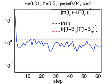
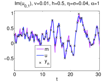
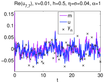
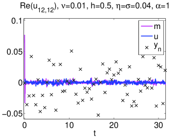
Figure 1: Example of a stable trajectory for 3DVAR with $\nu=0.01,h=0.5,\eta=\sigma=0.04,\alpha=1$. The top left plot shows the norm-squared error between the estimated mean, $m(t_{n})=\hat{m}_{n}$, and the signal, $u(t_{n})$, in comparison to the preferred upper bound (i.e. the total observation error ${\rm tr}(\Gamma)=\Xi$) and the lower bound ${\rm tr}[(I-B_{n})\Gamma(I-B_{n})]$. The other three plots show the estimator, $m(t)$, together with the signal, $u(t)$, and the observations, $y_{n}$ for a few individual modes.

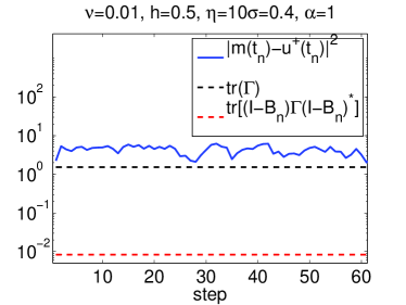
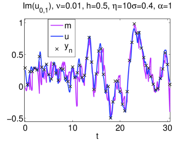
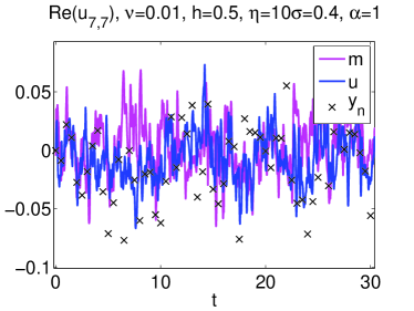
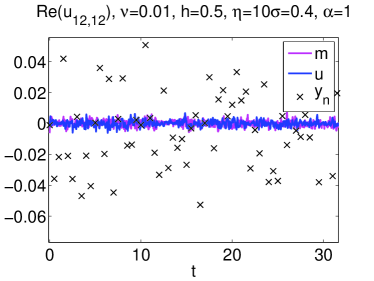
Figure 2: Example of a destabilized trajectory for 3DVAR with the same parameters as in Fig. 1 except the larger value of $\eta=10\sigma=0.4$. Panels are the same.

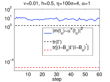
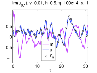
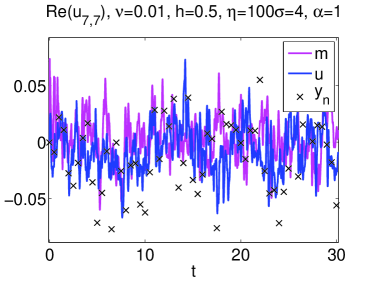
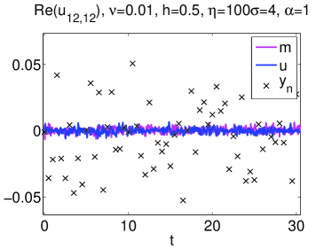
Figure 3: Example of a destabilized trajectory for 3DVAR with the same parameters as in Fig. 1 except the larger value of $\eta=100\sigma=4$. Panels are the same.

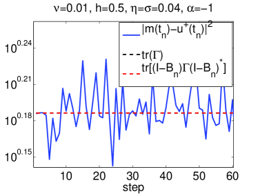
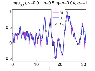
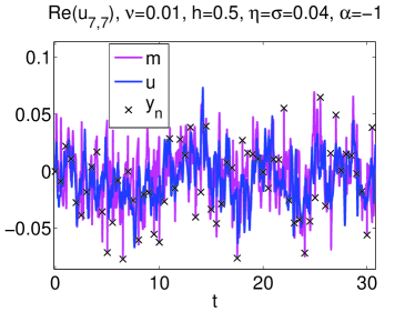
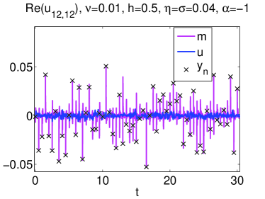
Figure 4: Example of a stable trajectory for 3DVAR with the same parameters as in Fig. 1 except with $\alpha=-1$. Panels are the same.

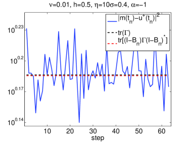
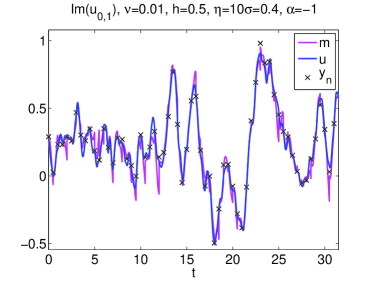
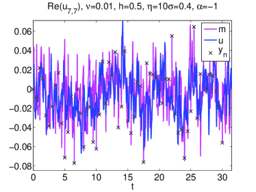
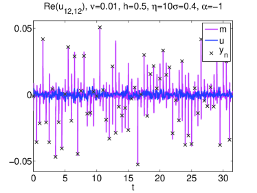
Figure 5: Example of a stable trajectory for 3DVAR with the same parameters as in Fig. 2 except with value of $\alpha=-1$. Panels are the same.

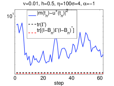
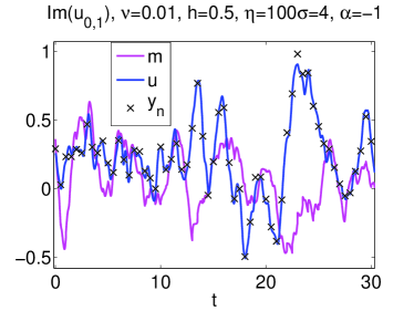
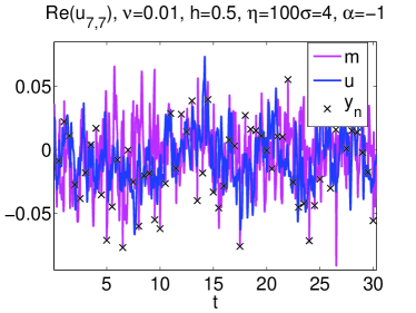
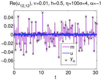
Figure 6: Example of a destabilized trajectory for 3DVAR with the same parameters as in Fig. 3 except with value of $\alpha=-1$. Panels are the same.

5.4 Partial Observations; Discrete Time

We now proceed to examine the case of partial observations, illustrating Theorem 4.3. Note that the forced mode has magnitude $|k_{f}|^{2}=50$, so ensuring that it is observed requires that $\lambda>50\lambda_{1}$. When enough modes are retained, for example when $\lambda=100\lambda_{1}$ in our setting, the results for the $\alpha=1$ case remain roughly the same and are not shown. However, in the case $\alpha=-1$, in which the observations are trusted more than the model at high wavevectors, the results are greatly improved by ignoring the observations of the high-frequencies. See Fig. 7. This improvement, and indeed the improvement beyond setting $B=0$ for both cases $\alpha=\pm 1$ disappears as $\lambda$ is decreased. In particular, when $\lambda=25\lambda_{1}$ the error is never very much smaller than the upper bound. This is due to the fact that the dynamics of the low wavevectors tend to be unpredictable and they contain very little useful information for the assimilation. Then, for much smaller $\lambda=4\lambda_{1}$, once enough unstable modes are left unobserved, there is no convergence. The order of magnitude of the error in the asymptotic regime as a function of $\eta$ remains roughly consistent as $\lambda$ is decreased until the estimator no longer converges. For small $h$ (high-frequency in time observations) and complete observations, the estimator can be slow to converge to the asymptotic regime. In this case, the number of iterations until convergence, for a sufficiently small $\eta$, becomes significantly larger as $\lambda$ is decreased (again until the estimator fails to converge at all).

Given $\lambda\approx k_{\lambda}^{2}\lambda_{1}$, we expect that for $\eta$ sufficiently small the contribution of the model to the filter will be negligible for all $k$ with $|k|<k_{\lambda}$ for $\alpha=1$. Hence the estimators for both $\alpha=\pm 1$ will behave similarly. An example of this is shown in Fig. 8 where $\eta=0.01\sigma=0.0004$ and $\lambda=49\lambda_{1}$ in Fig. 8. In both cases, the estimator is essentially utilizing all the available observations. There are enough observations to draw the higher wavevectors of the estimator closer to the truth than if we just set the population of those modes to zero. In contrast, as mentioned above, when $\lambda=25\lambda_{1}$, there are not enough observations even when they are all used, and the error is roughly the same as the upper bound as $\eta\rightarrow 0$ (not shown).

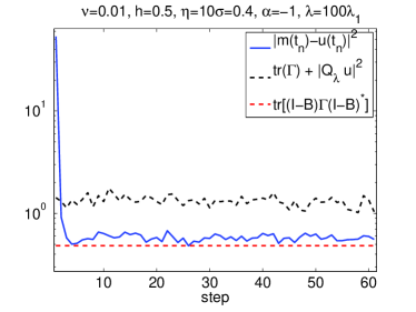
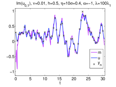
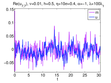
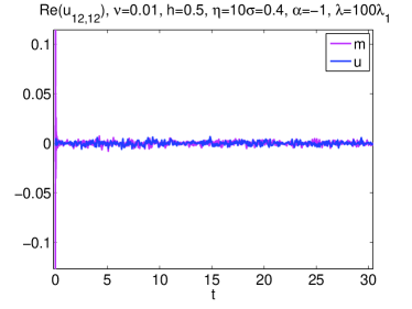
Figure 7: Example of an improved estimator for partial observations with $\lambda=100\lambda_{1}$ and otherwise the same parameters as in Fig. 5. Panels are the same.

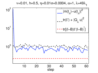
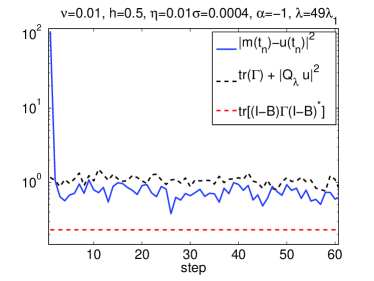
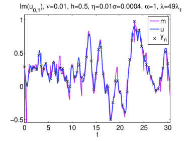
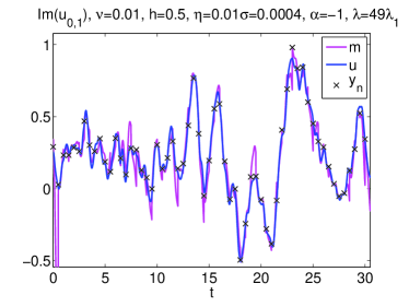
Figure 8: Examples of estimators for partial observations with $\lambda=49\lambda_{1}^{2}$ and $\eta=0.1\sigma=0.004$, otherwise the same parameters as in Figs. 1 and 4. Left panels are for $\alpha=1$ and right panels are for $\alpha=-1$.

5.5 Continuous Observations

Finally, we explore the case of continuous observations using the SPDE and PDE derived in subsection 4.4. We let $\alpha=1/2$ throughout. We invoke a split-step scheme to solve Eqns. 38 and 39 in which we compose solutions of (3) and the Ornstein-Uhlenbeck process

$$\frac{\mathrm{d}\widehat{m}}{\mathrm{d}t}+\omega A_{0}^{-2\alpha}(\widehat{m}-u)=\omega\sigma_{0}A_{0}^{-2\alpha-\beta}\frac{\mathrm{d}W}{\mathrm{d}t},\quad\widehat{m}(0)=\widehat{m}_{0},$$ (43)

at each step, when $r=1$, and setting $\sigma_{0}=0$ in (43) when $r<1$. We begin by considering the $r=1$ case in which we recover the SPDE (38). Notice that the parameter $\omega$ sets a time-scale for relaxation towards the true signal, and $\sigma_{0}$ sets a scale for the size of flucuations about the true signal. The parameter $\beta$ rescales the fluctuation size at different wavevectors with respect to the relaxation time. First we consider setting $\beta=0.$ In Fig. 9 we show numerical experiments with $\omega=100$ and $\sigma_{0}=0.05.$ We see that the noise level on top of the signal in the low modes is almost $O(1)$, and that the high modes do not synchronize at all; the total error remains $O(1)$ although trends in the signal are followed. On the other hand, for the smaller value of $\sigma_{0}=0.005$, still with $\omega=100$, the noise level on the signal in the low modes is moderate, the high modes synchronize sufficiently well, and the total error is small. See Fig. 10.

Now we consider the case $\beta=1$. Again we take $\omega=100$ and $\sigma_{0}=0.05$ and $0.005$ in Figures 11 and 12, respectively. The synchronization is stronger than that observed for $\beta=0$ in each case. This is because the noise decays more rapidly for large wavevectors when $\beta$ is increased, as can be observed in the relatively smooth trajectories of the high modes of the estimator.

For the case when $r<1$ and we recover a PDE, the values of $\sigma_{0}$ and $\beta$ are irrelevant. The value of $\omega$ is the critical parameter in this case. For values of $\omega$ of $O(100)$ the convergence is exponentially fast to machine precision. For values of $\omega$ of $O(1)$ the estimator does not exhibit stable behviour. For intermediate values, the estimator may approach the signal and remain bounded and still an $O(1)$ distance away(see the case $\omega=10$ in Fig. 13), or else it may come close to synchronizing (see the case $\omega=30$ in Fig. 14).

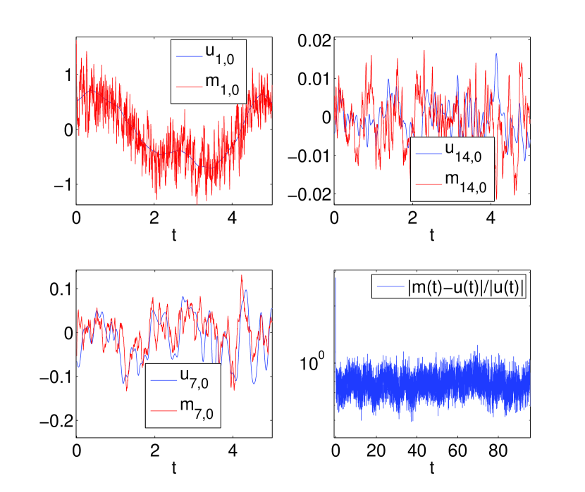
Figure 9: Trajectories of various modes of the estimator $\widehat{m}$ and the signal $u$ are depicted above for $\beta=0$ and $\sigma_{0}=0.05$, along with the total relative error in the $l^{2}$ norm, $|\widehat{m}-u|/|u|$.

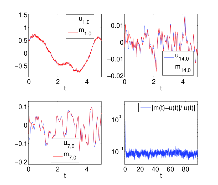
Figure 10: Trajectories of various modes of the estimator $\widehat{m}$ and the signal $u$ are depicted above for $\beta=0$ and $\sigma_{0}=0.005$, along with the relative error.

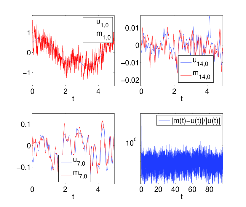
Figure 11: Trajectories of various modes of the estimator $\widehat{m}$ and the signal $u$ are depicted above for $\beta=1$ and $\sigma_{0}=0.05$, along with the relative error.

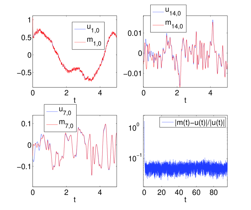
Figure 12: Trajectories of various modes of the estimator $\widehat{m}$ and the signal $u$ are depicted above for $\beta=1$ and $\sigma_{0}=0.005$, along with the relative error.

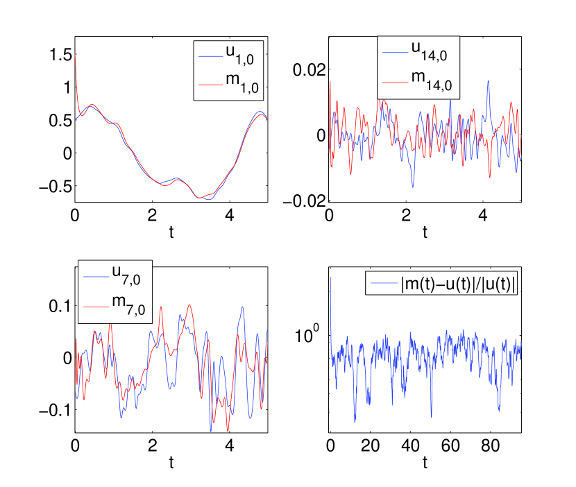
Figure 13: Trajectories of various modes of the estimator $\widehat{m}$ and the signal $u$ are depicted above for $r<1$ and $\omega=10$, along with the relative error.

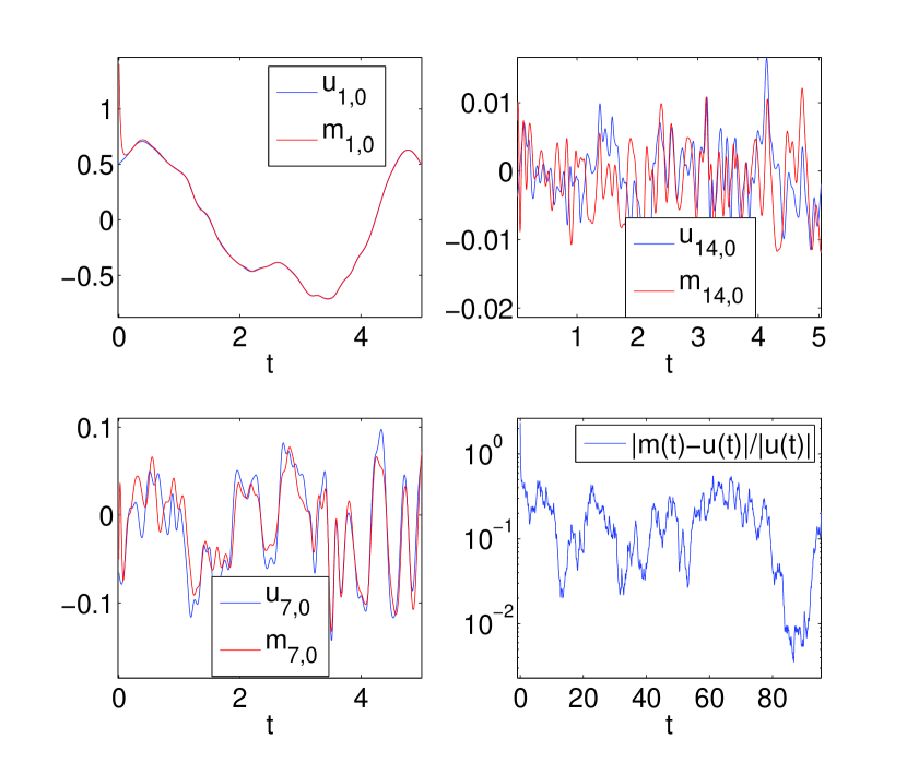
Figure 14: Trajectories of various modes of the estimator $\widehat{m}$ and the signal $u$ are depicted above for $r<1$ and $\omega=30$, along with the relative error.

6 Conclusion

This paper contains three main components:

• we show that the filtering problem for the Navier-Stokes equation may be formulated as a well-posed inverse problem in function space, and demonstrated how various approximate Gaussian filters can be derived (Theorems 3.2 and 3.5, and Corollary 3.3);

• we prove Theorems 4.3 and 4.7, which establish filter stability for small enough observational noise;

• we derive an SPDE (38) and a PDE (39), which may be used as the basis to study filter stability in the case of frequent observations and large observational noise.

Numerical results are used to illustrate, and extend the validity of, the theory.

There are a number of natural future directions which stem from this work:

• to develop analogous filter stability theorems for more sophisticated filters, such as the extended and ensemble-based methods, when applied to the Navier-Stokes equation;

• to rigorously derive, and study the properties of, the SPDE (38) which characterizes filter stability in the case of frequent observations and large observational noise;

• to study model-data mismatch by looking at filter stability for data generated by forward models which differ from those used to construct the filter;

• to study the effect of filtering in the presence of model error, by similar methods, to understand how this may be used to overcome problems arising from model-data mismatch.

Acknowledgements AMS would like to thank the following institutions for financial support: EPSRC, ERC and ONR; KJHL was supported by EPSRC and ONR; and CEAB, KFL, DSM and MRS were supported EPSRC, through the MASDOC Graduate Training Centre at Warwick University. The authors also thank The Mathematics Institute and Centre for Scientific Computing at Warwick University for supplying valuable computation time. Finally, the authors thank Masoumeh Dashti for valuable input.

References

- [1] A. Bain and D. Crişan. Fundamentals of Stochastic Filtering. Springer Verlag, 2008.
- [2] A. Carrassi, M. Ghil, A. Trevisan, and F. Uboldi. Data assimilation as a nonlinear dynamical systems problem: Stability and convergence of the prediction-assimilation system. Chaos: An Interdisciplinary Journal of Nonlinear Science, 18:023112, 2008.
- [3] A. Chorin, M. Morzfeld, and X. Tu. Implicit particle filters for data assimilation. Communications in Applied Mathematics and Computational Science, page 221, 2010.
- [4] P. Constantin and C. Foiaş. Navier-Stokes equations. University of Chicago Press, 1988.
- [5] S. L. Cotter, M. Dashti, J. C. Robinson, and A. M. Stuart. Bayesian inverse problems for functions and applications to fluid mechanics. Inverse Problems, 25(11):115008, 43, 2009.
- [6] P. Courtier, E. Andersson, W. Heckley, D. Vasiljevic, M. Hamrud, A. Hollingsworth, F. Rabier, M. Fisher, and J. Pailleux. The ECMWF implementation of three-dimensional variational assimilation (3d-Var). I: Formulation. Quart. J. R. Met. Soc., 124(550):1783–1807, 1998.
- [7] SM Cox and PC Matthews. Exponential time differencing for stiff systems. Journal of Computational Physics, 176(2):430–455, 2002.
- [8] A. Doucet, N. De Freitas, and N. Gordon. Sequential Monte Carlo methods in practice. Springer Verlag, 2001.
- [9] G. Evensen. Data Assimilation: the Ensemble Kalman Filter. Springer Verlag, 2009.
- [10] M. Hairer and J.C. Mattingly. Ergodicity of the 2D Navier-Stokes equations with degenerate stochastic forcing. Annals of Mathematics, 164:993–1032, 2006.
- [11] J. Harlim and AJ Majda. Filtering nonlinear dynamical systems with linear stochastic models. Nonlinearity, 21:1281, 2008.
- [12] A.C. Harvey. Forecasting, Structural Time Series Models and the Kalman filter. Cambridge Univ Pr, 1991.
- [13] K. Hayden, E. Olson, and E.S. Titi. Discrete data assimilation in the Lorenz and 2d Navier-Stokes equations. Physica D: Nonlinear Phenomena, 2011.
- [14] J.S. Hesthaven, S. Gottlieb, and D. Gottlieb. Spectral Methods for Time-Dependent Problems, volume 21. Cambridge Univ Pr, 2007.
- [15] K.J.H. Law and A.M. Stuart. Evaluating data assimilation algorithms. Arxiv preprint arXiv:1107.4118, 2011.
- [16] A. C. Lorenc. Analysis methods for numerical weather prediction. Quart. J. R. Met. Soc., 112(474):1177–1194, 2000.
- [17] A. C. Lorenc, S. P. Ballard, R. S. Bell, N. B. Ingleby, P. L. F. Andrews, D. M. Barker, J. R. Bray, A. M. Clayton, T. Dalby, D. Li, T. J. Payne, and F. W. Saunders. The Met. Office global three-dimensional variational data assimilation scheme. Quart. J. R. Met. Soc., 126(570):2991–3012, 2000.
- [18] A. Majda and X. Wang. Non-linear dynamics and statistical theories for basic geophysical flows. Cambridge Univ Pr, 2006.
- [19] A.J. Majda, J. Harlim, and B. Gershgorin. Mathematical strategies for filtering turbulent dynamical systems. Dynamical Systems, 27(2):441–486, 2010.
- [20] E. Olson and E.S. Titi. Determining modes for continuous data assimilation in 2D turbulence. Journal of statistical physics, 113(5):799–840, 2003.
- [21] D. F. Parrish and J. C. Derber. The national meteorological center’s spectral statistical-interpolation analysis system. Monthly Weather Review, 120(8):1747–1763, 1992.
- [22] J. C. Robinson. Infinite-Dimensional Dynamical Systems. Cambridge Texts in Applied Mathematics. Cambridge University Press, Cambridge, 2001.
- [23] T. Snyder, T. Bengtsson, P. Bickel, and J. Anderson. Obstacles to high-dimensional particle filtering. Monthly Weather Review., 136:4629–4640, 2008.
- [24] A. M. Stuart. Inverse problems: a Bayesian perspective. Acta Numer., 19:451–559, 2010.
- [25] R. Temam. Navier-Stokes Equations and Nonlinear Functional Analysis. Number 66. Society for Industrial Mathematics, 1995.
- [26] R. Temam. Infinite-Dimensional Dynamical Systems in Mechanics and Physics, volume 68 of Applied Mathematical Sciences. Springer-Verlag, New York, second edition, 1997.
- [27] Z. Toth and E. Kalnay. Ensemble forecasting at NCEP and the breeding method. Monthly Weather Review, 125:3297, 1997.
- [28] P.J. Van Leeuwen. Particle filtering in geophysical systems. Monthly Weather Review, 137:4089–4114, 2009.
- [29] PJ van Leeuwen. Nonlinear data assimilation in geosciences: an extremely efficient particle filter. Quarterly Journal of the Royal Meteorological Society, 136(653):1991–1999, 2010.