The complementarity of the redshift drift

We derive some basic equations related to the redshift drift and we show how some dark energy (DE) properties can be retrieved from it. We consider in particular three kinds of DE models which exhibit a characteristic signature in their redshift drift while no such signature would be present in their luminosity-distances: a sudden change of the equation of state parameter $w_{DE}$ at low redshifts, oscillating DE and finally an equation of state with spikes at low redshifts. Accurate redshift drift measurements would provide interesting complementary probes for some of these models and for models with varying gravitational coupling. While the redshift drift would efficiently constrain models with a spike at $z\sim 1$, the signature of the redshift drift for models with large variations at very low redshifts $z<0.1$ would be unobservable, allowing a large arbitrariness in the present expansion of the universe.

PACS Numbers: 04.62.+v, 98.80.Cq

1 Introduction

Data suggests that our universe has entered a stage of accelerated expansion rate. This is a radical departure from conventional cosmology in which the expansion was constantly decelerated except for the inflationary stage in the very early universe. The mechanism behind this late-time accelerated expansion is unclear and many models were suggested [1]. If it is caused by some isotropic perfect fluid component called dark energy (DE) while gravity is governed by General Relativity (GR), then DE should make up about two thirds of the universe content. The simplest possibility, a cosmological constant $\Lambda$ is problematic from the theoretical point of view because of its tiny amplitude. Further while the data is in agreement with a cosmological constant $\Lambda$, the precision of these data do not allow to rule out models where the equation of state (EoS) parameter of the dark energy component $w_{DE}$ differs from $-1$ and varies with time, and in which the corresponding energy density depends on time as well. A great number of models have been proposed and all their properties were intensively investigated in the hope that future accurate observations would allow to discriminate between these models and that only a small part of them would remain as viable candidates while the other models would be ruled out. Another attractive possibility is a modification of gravity on cosmic scales. Virtually all the foundations of standard cosmology have been questioned in the quest for a solution to the dark energy problem. Decisive progress in settling the issue will come from observations. Experiments of different kinds are planned that will probe with exquisite precision the universe background expansion and also the evolution of the perturbations.

To make progress in the understanding of the nature of DE it is desirable to explore all ways in which its properties can be probed. One such probe is the redshift drift. The feasibility of such measurements was reassessed in [2], many years after its theoretical discovery [3]. It has been suggested recently as a way to test general properties of the DE paradigm [4]. These measurements could give additional insight into the properties of DE because they probe directly the quantity $H(z)$. It is this aspect that we want to emphasize and to investigate in this work. Before embarking on the quantitative assessment of redshift drift data for some specific models we first derive some general properties of the redshift drift relevant for the study of DE.

2 The redshift drift

In an expanding universe many physical quantities evolve with time. The redshift suffered by radiation emitted by a source depends on time as well. Indeed let us consider radiation emitted by a source at the emission time $t_{e}$. If this radiation is observed at time $t_{0}$, the corresponding redshift is given by

$$1+z(t_{e},t_{0})=\frac{a(t_{0})}{a(t_{e})}\equiv\frac{a_{0}}{a_{e}}~{},$$ (1)

where we use the notation $z(t_{e},t_{0})$ to emphasize that the redshift depends on the emission time $t_{e}$ and on the observation time $t_{0}$. If radiation emitted by the same source is observed at time $t_{0}+\delta t_{0}$, the redshift will change by an amount $\delta z$

$$\delta z\equiv z(t_{e}+\delta t_{e},t_{0}+\delta t_{0})-z(t_{e},t_{0})~{}.$$ (2)

It is easy to derive the following expression

$$\delta z = \frac{\delta t_{0}}{a_{e}}\left(\dot{a}_{0}-\dot{a}_{e}\right)$$ (3)

$$= H_{0}\delta t_{0}\left(1+z(t_{e},t_{0})-h_{e}\right)~{}~{}~{}~{}~{}~{}~{}~{}~{}~{}h_{e}\equiv\frac{H_{e}}{H_{0}}$$ (4)

$$= H_{0}\delta t_{0}\left(1+z-h(z)\right)$$ (5)

with the obvious notation $H_{e}=H(t_{e})$. We have dropped the subscript $e$ and finally we return to more conventional notations setting $z\equiv z(t_{e},t_{0})$. It is obvious from (3) that $\delta z$ is a decreasing negative function of $z$ in a universe whose expansion rate is always decelerated. This is what would happen e.g. for an Einstein-de Sitter universe. However the situation changes when at least part of the expansion is accelerated. Let us consider a universe for which the deceleration parameter $q$ satisfies $q<0$ for $z<z_{q}$ and $q>0$ for $z>z_{q}$ and $q(z_{q})=0$. This is the case for a flat universe with dust-like matter and a cosmological constant $\Lambda$ satisfying $\Omega_{\Lambda,0}>\frac{1}{3}$. For this universe we see from (3) that $\delta z$ must be an increasing function of $z$ on the interval $z<z_{q}$ during which the expansion rate is accelerating. At large redshifts, when the expansion rate is decelerating (and matter-dominated), $\delta z$ will decrease in function of $z$. Note that $\delta z$ vanishes in a Milne (empty) universe.

It is interesting to study this behaviour by considering the slope $(\delta z)^{\prime}\equiv\frac{d}{dz}\left(\delta z\right)$. We have

$$(\delta z)^{\prime}=H_{0}\delta t_{0}\left(1-h^{\prime}\right)~{}.$$ (6)

The slope is positive for $h^{\prime}<1$ and negative for $h^{\prime}>1$. For a universe with accelerated expansion rate on the interval $0\leq z\leq z_{q}$, $\delta z$ reaches its maximum at $z_{m}$ when $h^{\prime}(z_{m})=1$. One can show that we have $z_{m}>z_{q}$ with $z_{m}$ typically only slightly larger than $z_{q}$. We will consider below even more sophisticated scenarios where the slope is first negative at $z=0$, then positive at higher $z$ in order to ensure a late-time accelerated stage and then again negative. It is convenient to introduce the new dimensionless quantity

$$\Delta z\equiv\frac{\delta z}{H_{0}\delta t_{0}}~{}.$$ (7)

It is easy to derive the following equalities

$$1+q = \frac{1-(\Delta z)^{\prime}}{1-\frac{\Delta z}{1+z}}=\frac{3}{2}(1+w_{\rm eff})$$ (8)

$$w_{DE} = \left[\frac{1-(\Delta z)^{\prime}}{\frac{3}{2}\left(1-\frac{\Delta z}{1+z}\right)}-1\right]\left[1-\frac{\Omega_{m,0}(1+z)}{\left(1-\frac{\Delta z}{1+z}\right)^{2}}\right]^{-1}~{},$$ (9)

where spatial flatness is assumed in (9). When we use luminosity distances, second derivatives are necessary. We have in particular

$$(\Delta z)^{\prime}_{0}=-q_{0}~{}.$$ (10)

In contrast to the luminosity distance $d_{L}(z)$, the leading order of $\delta z$ for $z\ll 1$ is model dependent and allows to discriminate between models with same $H_{0}$ but different $q_{0}$. Physically this is so because the slope at $z=0$ is sensitive to the dark energy EoS as we see from eqs.(8,9). Note that at the redshift $z_{1}\neq 0$ where $\delta z=0$ (if it exists), $(\Delta z)^{\prime}=-q$. The following inequality

$$(\Delta z)^{\prime}>1~{},$$ (11)

is satisfied by a universe on all redshifts for which it is in a phantom phase, $q<-1$ or $w_{\rm eff}=\Omega_{DE}~{}w_{DE}<-1$. Hence a universe in a phantom phase on small redshifts must satisfy inequality (11) on these redshifts. If it is DE itself which is of the phantom type, $w_{DE}<-1$, the following weaker inequality has to be satisfied

$$(\Delta z)^{\prime}>1-\frac{3}{2}\frac{\Omega_{m,0}(1+z)^{2}}{1+z-\Delta z}~{}.$$ (12)

When DE is a cosmological constant $\Lambda$, the above inequality becomes a strict equality. Note that $(\Delta z)^{\prime}=1$ in a de Sitter universe which corresponds to the asymptotic future of a flat universe with a cosmological constant $\Lambda$ ($\Omega_{m}\to 0$).

These properties can be seen with the small-$z$ expansion

$$\Delta z=-\left[q_{0}z-\frac{1}{2}(q^{2}_{0}-j_{0})z^{2}+...\right]~{},$$ (13)

which is to be contrasted with the expansion

$$D_{L}(z)\equiv H_{0}~{}d_{L}(z)=z+\frac{1}{2}(1-q_{0})z^{2}+...$$ (14)

The leading term of (14) is the same for all models with identical $H_{0}$ in contrast to (13). The result (10) is obviously recovered from (13). In (13) $j_{0}$ is the “jerk” parameter, $j=\frac{\dddot{a}}{aH^{3}}$, at z=0. Expression (13) shows also how $\Delta z$ deviates from a linear law at small redshifts. From (13), this deviation is positive i.e.

$$\Delta z>-q_{0}z~{},~{}~{}~{}~{}~{}~{}~{}~{}~{}~{}~{}~{}~{}~{}~{}~{}~{}~{}~{}~{}~{}~{}z>0,~{}z\approx 0$$ (15)

on some small interval around $z=0$ when the acceleration is slowing down on small redshifts. These properties of the redshift drift are illustrated with Figure 1.

Let us return finally to the amplitude of the redshift drift. Clearly it is proportional to the small quantity $H_{0}\delta t_{0}$. In other words all equations and inequalities derived above make use of $\Delta z$, the redshift drift in units $H_{0}\delta t_{0}$. For $\delta t_{0}=N$ years, $H_{0}\delta t_{0}=1.023~{}N~{}h\times 10^{-10}$ (here $h=H_{0}/100km/sMpc$), so $\delta t_{0}$ should be at least of the order of $10$ years to yield a measurable effect. We will consider in the next section some specific models.

3 Models with peculiar equation of state

We consider now various DE models exhibiting a characteristic signature in their redshift drift because the equation of state (EoS) parameter $w_{DE}$ has a special behaviour on low redshifts. The choice of models in this study looked for distinctive features.

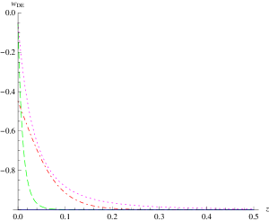
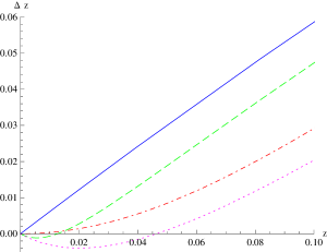
Figure 1: a) On the left panel, three models are displayed with a large variation of $w_{DE}$ on low redshifts. In these universes the acceleration is slowing down on low redshifts and the expansion is even decelerating on very low redshifts for the top (pink) and bottom (green) curves. The red curve (in the middle) is taken from [8] and has $q_{0}\approx 0$. b) On the right panel the corresponding redshift drifts are displayed. The blue curve corresponds to a $\Lambda$CDM universe. Note that the other three curves satisfy the inequality (15). The corresponding luminosity distances have no characteristic signatures though the pink curve is in tension with SNIa data while the model with the green curve provides an excellent fit because strong variation of $w_{DE}$ for this model, with presently decelerated expansion, is confined to the interval $z\leq 0.1$.

3.1 Large variation of $w_{DE}$ on low redshifts

We start with models with a large variation of $w_{DE}$ starting from very low redshifts and on until today. There are several situations where such a variation can occur, for example in models where the accelerated stage is transient and the accelerated expansion is already slowing down on very low redshifts. This can be the case for some quintessence models (see e.g. [5],[6]) or for more exotic models with a singularity in the future (see e.g. [7]). It was also proposed recently as an interesting phenomenological ansatz that can improve the fit to SNIa data compared to a pure cosmological constant [8]. Three models are shown on Figure 1. We see that these models have a characteristic slope of their redfshift drift at very low redshifts which differs significantly from the slope obtained for $\Lambda$CDM $(\Delta z)^{\prime}=1-\frac{3}{2}\frac{\Omega_{m,0}(1+z)^{2}}{1+z-\Delta z}$. The slope at $z=0$ is negative if the universe is presently decelerating and rapid variation of $w_{DE}$ produces a sharp change in $\delta z$. Redshift drift measurements on such very low redshifts suffer from increased difficulties related to the peculiar velocities of objects and are virtually impossible. While the signatures of the models considered in this subsection are most probably not observable, they illustrate nicely the results derived in section 2. As a substantial amount of SNIa data have been added in the interval $0.1\leq z\leq 0.4$ in the Union2 set as compared to the Constitution set, two of these models are now in tension with SNIa data. The model with the pink curve on Figure 1 (denoted mod2 in Table 1) is in tension with the data because it departs from $w_{DE}=-1$ on higher redshifts $z<0.5$. However the model with the green curve in Figure 1 (denoted mod1 in Table 1) provides an excellent fit to the data. It has a sharp departure from $w_{DE}=-1$ on redshifts $z<0.1$ only and a decelerated expansion today. This is in agreement with results obtained in [9].

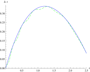
Figure 2: a) The redshift drift for several models with a “spike” in their EoS parameter $w_{DE}$ is shown on the left panel. The spikes located at $z=0.2$ (red and green curves) have identical widths and amplitudes (maximal heighths) $A_{sp}=0.5$ and $A_{sp}=0.2$ respectively. The third spike at $z=1$ (pink curve) has a larger width and amplitude $A_{sp}=0.7$. The location and amplitude of the spike leaves a neat signature in the redshift drift. b) The redshift drift of $\Lambda$CDM and a model with oscillating $w_{DE}$ (with amplitude $A_{osc}=0.3$) are displayed on the right panel. The oscillations are clearly seen in the redshift drift while they are essentially erased in the luminosity distance.

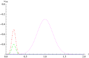
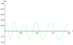
Figure 3: a) The equation of state parameters of our models with spike appearing in Figures 2 (same colour as in Figure 2) are shown on the left panel. b) On the right panel, the oscillating model used in Figure 2 is displayed.

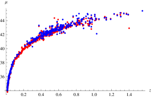
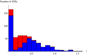
Figure 4: a) SNIa distance modulus data from the Constitution set (blue points) and Union2 set (red points). b) Number of supernovae per redshift intervals of 0.1 for the two data sets. There is a substantial addition in the Union2 data set in the interval $0.1\leq z\leq 0.4$, which accounts for the stronger constraints in models with modifications at low redshift.

3.2 Spikes in the equation of state

Here we consider models where $w_{DE}$ exhibits a spiky feature (see e.g. [9],[10]). The larger the redshift where a spike of given amplitude (i.e. maximal heighth) $A_{sp}$, and width is located, the smaller the effect on $\delta z$ because $\Omega_{DE}$ decreases with redshift and hence the effect on $H(z)$ of a spike in $w_{DE}$ will decrease as well. We consider models which have the same fiducial value $w_{DE,0}=-1$ with a superimposed spike.

We can have models with a clear signature of the spike indicating precisely its location because the slope of $\delta z$ depends directly on $w_{DE}$ and several models are displayed in Figure 2. In luminosity-distances the feature of the spike is erased by the integration so the effect can easily be degenerate with variations of other cosmological parameters and there is no signature which can be unambiguously attributed to the presence of a spike in the equation of state parameter $w_{DE}$. The red curve with a pronounced spike at $z=0.2$ (denoted Spike R in Table 1) is ruled out by SNIa data while the green curve with a less pronounced spike located at the same redshift is in tension with the data. On the other hand the model with a spike at $z=1$ (denoted Spike P in Table 1) provides a very good fit to the data. It is interesting to remark that, due to the reduced number of data at high redshifts, even a stronger modification in $w_{DE}$ like this one can go unnoticed if only SNIa and BAO data is used. From Figure 2, the difference in the quantity $10^{10}~{}\delta z$ between the SpikeP model and $\Lambda$CDM at $z\sim 2$ in a 15-years experiment is estimated to be about 1.2. As things stand now this is still too small to allow for a discrimination by a planned experiment like CODEX [14]. However an improvement of order 4 of the sensitivity would allow to distinguish both models.

3.3 Oscillating dark energy

Another possibility is provided by models where DE has an oscillating EoS parameter (see e.g. [15]), viz.

$$w_{DE}=-1+A_{osc}\sin\left[B\ln(1+z)+C\right]~{}.$$ (16)

Oscillations in $H(z)$ are induced but will be essentially erased in the luminosity-distances. In contrast these oscillations appear clearly in the redshift drift as models displayed on Figure 2 show. It is quite clear that a detection of these oscillations require very accurate data. These oscillations could be detected with accurate data on redshifts $z\sim 2$ in the range where one expects at least in principle accurate data to be possible.

	mod1	mod2	SSS	Spike R	Spike G	Spike P	Osc.	LCDM
$\Omega_{m,0}$	0.267	0.255	0.257	0.241	0.254	0.272	0.262	0.266
$\chi_{2}$	544.5	549.5	547.0	554.6	546.7	545.0	544.9	544.9

Table 1: Best-fit $\Omega_{m,0}$ and $\chi^{2}$ values after marginalization of $H_{0}$, using the Union2 set [11] of 557 SN Ia, the BAO distance ratio [12] and the CMB shift parameter [13]. The first three models correspond resp. to the green, pink and red curves of Figure 1. The models Spike R, Spike G and Spike P correspond resp. to the red, green and pink curves of Figure 2a. There are now enough SNIa data on low redshifts to put most of the models with a large variation of $w_{DE}$, or a pronounced feature, on very low redshifts either in tension with the data (Spike G, SSS) or even to rule out some of them (Spike R, mod2). Redshift drift on these low redshifts would be virtually impossible to measure. But other models are viable and could be potentially constrained using the redshift drift. In particular, Spike P is a strong modification at large redshifts while fitting the data almost as well as $\Lambda$CDM.

4 Some models beyond General Relativity

In this section we would like to show that redshift drift measurements could help in some cases to establish whether a model is inside General Relativity (GR) or outside it. We have in mind models outside GR for which the gravitational constant defining the Chandrasekhar mass evolves with time so that the intrinsic luminosity of SNIa would not be constant for such models. We caution that there are many modified gravity models where this is not the case because the gravitational constant around compact objects is constant and basically equal to the usual Newton’s constant (see [16] for a related discussion in the context of some viable $f(R)$ DE models).

For our discussion it is sufficient to consider spatially flat universes. Let us assume that the intrinsic luminosity of SNIa has some redshift dependence

$$L(z)=L_{0}~{}{\cal G}(z)~{}~{}~{}~{}~{}~{}~{}~{}~{}~{}~{}~{}~{}~{}~{}~{}~{}~{}~{}~{}~{}~{}~{}~{}{\cal G}(z=0)=1.$$ (17)

In principle this could also arise for physical reasons unrelated to modifications of gravity (see e.g.[17]), but we will have in mind DE models where the variation of $L$ is induced by the variation of the gravitational constant defining the Chandrasekhar mass. For example (17) would occur in some models with varying gravitational coupling (see e.g. [18]) and in scalar-tensor models.

From (17), the expression for the measured flux ${\cal F}$ of SNIa can be written as

$${\cal F}=\frac{L(z)}{4\pi d^{2}_{L}}=\frac{L_{0}}{4\pi{\cal D}^{2}_{L}}~{},$$ (18)

where we have introduced the quantity

$${\cal D}_{L}=d_{L}~{}{\cal G}^{-\frac{1}{2}}~{}.$$ (19)

Measuring the flux ${\cal F}$ does not allow to disentangle the expansion of the universe from the variation of the intrinsic luminosity. One can only recover from SNIa data the quantity ${\cal D}_{L}(z)$.

Confusing the two quantities $d_{L}$ and ${\cal D}_{L}$ would lead to an erroneous retrieval of the background expansion because $H^{-1}(z)\neq\left(\frac{{\cal D}_{L}(z)}{1+z}\right)^{\prime}$. We have instead the equality

$$\left(\frac{{\cal D}_{L}}{1+z}\right)^{\prime}={\cal G}^{-\frac{1}{2}}~{}\left[H^{-1}+\frac{d_{L}}{1+z}\left(\ln{\cal G}^{-\frac{1}{2}}\right)^{\prime}\right]~{}.$$ (20)

Measuring $H(z)$, and hence indirectly also $d_{L}(z)$, from the redshift drift allows us to check whether one has ${\cal G}\neq 1$ and also provides us with information about the behaviour of ${\cal G}(z)$.

In the rest of this Section we consider the specific case of (massless) scalar-tensor models. In this model, the usual Newton’s constant in the equation for the growth of perturbations (and in the Poisson equation) is replaced by the effective gravitational coupling constant $G_{\rm eff}(z)$, viz. [19]

$$h^{2}~{}\delta_{m}^{\prime\prime}+\left(\frac{(h^{2})^{\prime}}{2}-\frac{h^{2}}{1+z}\right)\delta_{m}^{\prime}=\frac{3}{2}(1+z)\frac{G_{\rm eff}(z)}{G}~{}\Omega_{m,0}~{}\delta_{m}~{}.$$ (21)

Knowing $H(z)$ and the perturbations $\delta_{m}(z)$, one can check whether these two functions are consistent within a given model. The quantity $G_{\rm eff,0}\equiv G_{\rm eff}(z=0)$ is the coupling constant measured in a Cavendish type experiment, its numerical value is therefore extremely close to $G$.

Taking into account the dependence of the Chandrasekhar mass on $G_{\rm eff}$ and assuming simple SNIa models, the peak luminosity turns out to be proportional to $(\frac{G_{\rm eff}}{G_{\rm{eff},0}})^{-\frac{3}{2}}$ and we have [20]

$${\cal G}(z)=\left(\frac{G_{\rm eff}}{G_{\rm{eff},0}}\right)^{-\frac{3}{2}}~{},$$ (22)

leading to the well-known modification of the distance modulus $\mu$

$$\mu=5\log{\cal D}_{L}+\mu_{0}=5\log d_{L}+\frac{15}{4}\log\left(\frac{G_{\rm eff}}{G_{\rm{eff},0}}\right)+\mu_{0}~{},$$ (23)

with $\mu_{0}=25+5~{}\log~{}\left(\frac{cH_{0}^{-1}}{{\rm Mpc}}\right)$. If the second term is unknown, we cannot retrieve $H(z)$ from $\mu$. On the other hand if it is ignored, i.e. identifying ${\cal D}_{L}$ with $d_{L}$, an incorrect $H(z)$ is obtained from the observed $\mu$. While ignoring this modification of $\mu$ may be enough to show at least an inconsistency with the growth of perturbations in $\Lambda$CDM, or more generally in GR with smooth non-interacting DE, it does not allow to infer the correct behaviour of the quantity $G_{\rm eff}(z)$ from the growth of perturbations. On the other hand, redshift drift measurements yield directly the quantity $H(z)$ independently of SNIa data. Combining with SNIa data on a range of redshifts where both data overlap, one can recover the behaviour of $G_{\rm eff}(z)$ in this interval applying (20). The growth of matter perturbations give a consistency check with

$$h^{2}=\frac{(1+z)^{2}}{\delta^{\prime 2}}\Biggl{[}\delta_{0}^{\prime 2}+3\Omega_{m,0}\int_{0}^{z}\frac{G_{\rm eff}}{G}\frac{\delta^{\prime}\delta}{1+z^{\prime}}dz^{\prime}\Biggr{]}~{}.$$ (24)

Additional properties of the growth of matter perturbations can be used as additional tests (see e.g. [21]). Finally, let us mention that a varying $G_{\rm eff}$ will also affect the width of the light curve which could also provide some information about the evolution of $G_{\rm eff}$.

5 Summary and conclusions

We have studied models for which accurate redshift drift data can exhibit distinctive features not present in luminosity-distances. We emphasize that another incentive to achieve accurate redshift drift measurements comes from some DE models outside GR where an evolving gravitational constant affects the intrinsic luminosity of SNIa. It is well-known that these models can be efficiently probed by checking whether the expansion rate $H(z)$ and the perturbations $\delta_{m}(z)$ are consistent with each other inside a given model. The redshift-drift gives a direct probe of $H(z)$ independently of the modifications of gravity in contrast to SNIa data and we have illustrated this with scalar-tensor DE models. The expansion rate on very low redshifts can also be probed with Baryon Acoustic Oscillations (BAO) (see e.g. [22]) which rely on the nature and the evolution of matter perturbations. Systematics as well as the probed range of redshifts are different, so the two methods would be complementary. It is interesting that models with a strong variation of their EoS both on redshifts $z\leq 0.1$ and $z\sim 1$ would probably escape all observations which leaves some uncertainty about the present and future evolution of our universe (see for example ourmod1 and Spike P). Modifications at high redshifts, in particular, are poorly constrained by current data but can be potentially probed by redshift drift measurements.

We caution that the effect is tiny and that it is not clear yet whether it could be measured with the required accuracy. This obviously represents a technological challenge. However, as the exquisite data of the Cosmic Microwave Background anisotropy have spectacularly shown (see e.g. [13]), technological progress could make such measurements possible. If this is the case, redshift drift data could become useful as a complementary probe in order to help unveil the nature of DE especially if DE is of the kind investigated here.

References

- [1] V. Sahni, A. A. Starobinsky, Int. J. Mod. Phys. D9, 373 (2000); T. Padmanabhan, Phys. Rep. 380, 235 (2003); E. J. Copeland, M. Sami and S. Tsujikawa, Int. J. Mod. Phys. D15, 1753 (2006); V. Sahni, A. A. Starobinsky, Int. J. Mod. Phys. D15, 2105 (2006); S. Tsujikawa, arxiv:1004.1493
- [2] A. Loeb, Astrophys. J. 499, L111 (1998)
- [3] A. Sandage, Astrophys. J. 136, 319 (1962); G. McVittie, Astrophys. J. 136, 334 (1962).
- [4] A. Balbi, C. Quercellini, arXiv:0704.2350; M. Quartin, L. Amendola, Phys. Rev.D81, 043522 (2010); D. Jain, S. Jhingan, Phys. Lett. B692, 219 (2010); J.-P. Uzan, C. Clarkson, G. F.R. Ellis, Phys. Rev. Lett. 100, 191303 (2008).
- [5] D. Blais and D. Polarski, Phys. Rev. D 70, 084008 (2004).
- [6] S. Dutta, S.D.H. Hsu, D. Reeb, R. J. Scherrer, Phys. Rev. D 79 103504 (2009).
- [7] Z. Keresztes, L. Á. Gergely, V. Gorini, U. Moschella, A.Yu. Kamenshchik, Phys. Rev. D 79, 083504 (2009).
- [8] A. Shafieloo, V. Sahni, A. A. Starobinsky, Phys. Rev. D80, 101301 (2009).
- [9] M. Mortonson, W. Hu, D. Huterer, Phys. Rev. D80, 067301 (2009);
- [10] A. Hojjati, L. Pogosian, Gong-Bo Zhao, JCAP 1004, 007 (2010).
- [11] R. Amanullah et al., Astrophys. J. 716, 712 (2010).
- [12] W. J. Percival et al., MNRAS, 401, 2148 (2010).
- [13] E. Komatsu et al., Astrophys. J. Suppl. 192, 18 (2011).
- [14] V. D’Odorico on behalf of the CODEX/ESPRESSO team, arXiv:0708.1258.
- [15] E. Linder, Astropart. Phys. 25, 167 (2006); D. Jain, A. Dev, J. S. Alcaniz, Phys.Lett.B656, 15 (2007); S. Dutta, R. J. Scherrer, Phys. Rev. D78, 083512 (2008); J. Liu, H. Li, J. Xia, X. Zhang, JCAP 0907, 017 (2009); A. Kurek, O. Hrycyna, M. Szydlowski, Phys. Lett. B659, 14 (2008); Phys. Lett. B690, 337 (2010); R. Lazkoz, V. Salzano, I. Sendra, arXiv:1003.6084; L. Jarv, P. Kuusk, M. Saal, arXiv:1006.1246 .
- [16] R. Gannouji, B. Moraes and D. Polarski, JCAP 0902, 034 (2009).
- [17] S. Linden, J.-M. Virey, A. Tilquin, Astron.Astrophys.50, 1095 (2009)
- [18] I.L. Shapiro, J. Sola, H. Stefancic, JCAP 0501, 012 (2005).
- [19] B. Boisseau, G. Esposito-Farèse, D. Polarski and A.A. Starobinsky, Phys. Rev. Lett. 85, 2236 (2000).
- [20] L. Amendola, P. S. Corasaniti, F. Occhionero, astro-ph/9907222; E. Gaztanaga, E. Garcia-Berro, J. Isern, E. Bravo, I. Dominguez, Phys. Rev. D 65, 023506 (2002).
- [21] V. Acquaviva, L. Verde, JCAP 0712, 001 (2007); R. Gannouji, D. Polarski, JCAP 0805, 018 (2008); C. De Boni, K. Dolag, S. Ettori, L. Moscardini, V. Pettorino, C. Baccigalupi, arXiv:1008.5376 .
- [22] B. A. Bassett, R. Hlozek, in Dark Energy, Ed. P. Ruiz-Lapuente, Cambridge University Press (2010); arXiv:0910.5224.