Abstract

In this talk it is reported on an analysis [1] of the form factors for the transitions from a photon to one of the pseudoscalar mesons $\pi^{0},\eta,\eta^{\prime},\eta_{c}$ within the modified perturbative approach in which quark transverse degrees of freedom are retained. The report is focused on the discussion of the surprising features the new BaBar data exhibit, namely the sharp rise of the $\pi\gamma$ form factor with the photon virtuality and the strong breaking of flavor symmetry in the sector of pseudoscalar mesons.

1 Introduction

The recent measurements of the photon-to-pseudoscalar-meson transition form factors by the BaBar collaboration [2, 3, 4] has renewed the interest in these form factors. The BaBar data ruined the believe that these form factors are well understood in collinear QCD. The $\pi\gamma$ form factor in particular, measured up to about $35\,~{}{\rm GeV}^{2}$ now, reveals a sharp rise with the photon virtuality, $Q^{2}$. In fact, the scaled form factor $Q^{2}F_{\pi\gamma}$ approximately increases $\propto\sqrt{Q}$ which is in dramatic conflict with dimensional scaling and turned previous calculations based on collinear factorization obsolete - a substantial increase of the form factor is difficult to accommodate in fixed order perturbative QCD. For large $Q^{2}$ the form factor reads

$$Q^{2}F_{\pi\gamma}(Q^{2}) = \frac{\sqrt{2}f_{\pi}}{3}\,\int_{0}^{1}\,dx\,\Phi_{\pi}(x,\mu_{F})$$ (1)

$$\times \frac{1}{x}\,\Big{[}1+\frac{\alpha_{\rm s}(\mu_{R})}{2\pi}{\cal K}(x,\ln(Q^{2})\Big{]}\,.$$

The LO order result has been derived in [5], and the NLO result, ${\cal K}$, in [6]. In (1) $f_{\pi}$ is the familiar decay constant of the pion, $\mu_{F}$ and $\mu_{R}$ are the factorization and renormalization scales, respectively. The distribution amplitude, $\Phi_{\pi}$, or more generally that of a pseudoscalar meson, $P(=\pi^{0},\eta,\eta^{\prime})$, possesses a Gegenbauer expansion

$$\Phi_{P}(x,\mu_{F}) = \Phi_{\rm AS}\Big{[}1+\sum_{n=2,4,\cdots}a^{p}_{n}(\mu_{0})$$ (2)

$$\times \Big{(}\frac{\alpha_{\rm s}(\mu_{F})}{\alpha_{\rm s}(\mu_{0})}\Big{)}^{\gamma_{n}}C_{n}^{3/2}(2x-1)\Big{]}\,,$$

where the evolution of the expansion parameters, $a^{p}_{n}$, from an initial scale, $\mu_{0}$, to the factorization scale, $\mu_{F}$, is controlled by the anomalous dimensions $\gamma_{n}$ [5]. With $\mu_{F}\to\infty$ the distribution amplitude evolves in the asymptotic form $\Phi_{\rm AS}=6x(1-x)$. Obviously, (1) only provides $\log{Q^{2}}$ effects arising from the running of $\alpha_{\rm s}$ and the evolution of the distribution amplitude. Surprisingly, and this is in addition to the sharp rise of $F_{\pi\gamma}$ a second puzzle, the other transition from factors measured by the BaBar collaboration, namely $\eta\gamma$, $\eta^{\prime}\gamma$ and $\eta_{c}\gamma$, do not exhibit an anomalous $Q^{2}$ dependence, they behave as expected, see e.g. [7, 8].

Many theoretical papers have already been devoted to the interpretation of the BaBar data on the $\pi\gamma$ form factor. Limitation of space only allows to mention a few of them. Thus, for instance, the flat distribution amplitude, $\Phi_{\pi}\equiv 1$ has been proposed [9, 10] which, as is evident from (1), necessitates a regularization prescription for the infrared singular integral. This changes the asymptotic behavior of $Q^{2}F_{\pi\gamma}$ from the constant $\sqrt{2}f_{\pi}$ to $\propto\ln{Q^{2}}$. Other approaches base on light-cone sum rules [11, 12] or consider instanton effects [13]. Another possibility is to use ${\bf k}_{\perp}$-factorization instead of the collinear approach. Here, in this talk, it will be reported on an analysis [1] of the transition from factors on the basis of that factorization.

2 The transition form factors in ${\bf k}_{\perp}$-factorization

The basic idea of this approach is to retain the quark transverse degrees of freedom in the hard scattering. This however implies that quarks and antiquarks are pulled apart in the impact-parameter space, canonically conjugated to the transverse-momentum space. The separation of color sources is accompanied by the radiation of gluons. The corrections to the hard scattering process due to gluon radiation have been calculated in [14] in axial gauge using resummation techniques and having recourse to the renormalization group. These radiative corrections comprising resummed leading and next-to-leading logarithms which are not taken into account by the usual QCD evolution, are presented in the form of a Sudakov factor, $e^{-S}$. This approach, termed the modified perturbative approach (MPA), generates power corrections to the collinear result (1) which may explain the anomalous behavior of the BaBar data [1, 15]. According to [16] the form factor for a transition from a photon to a pseudoscalar meson (P) reads

$$F_{P\gamma}(Q^{2}) = \int dx\frac{d^{2}{\bf b}}{4\pi}\,\hat{\Psi}_{P}(x,-{\bf b},\mu_{F})$$ (3)

$$\times \hat{T}_{H}^{P}(x,{\bf b},Q,\mu_{R})e^{-S(x,b,Q,\mu_{R},\mu_{F})}$$

within the MPA. Since the Sudakov exponent $S$ is given in the impact-parameter space it is convenient to work in that space. In the convolution formula (3) $\hat{T}_{H}$ is the Fourier transform of the momentum-space hard scattering amplitude evaluated to lowest order perturbative QCD from the Feynman graphs displayed in Fig. 1

$$\hat{T}_{H}^{P}\,=\,\frac{2\sqrt{6}\,C_{P}}{\pi}\,K_{0}(\sqrt{x}Qb)\,.$$ (4)

Here $C_{P}$ is a charge factor. For instance, for the pion it reads $C_{\pi}=(e_{u}^{2}-e_{d}^{2})/\sqrt{2}$ where $e_{a}$ denotes the charge of a flavor-$a$ quark in units of the positron charge. The function $K_{0}$ denotes the modified Bessel function of order zero.

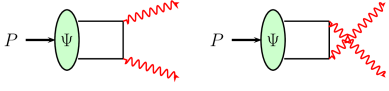
Figure 1: Lowest order Feynman graphs for the $P\gamma$ transition form factor.

The last item in (3) to be explained, is $\hat{\Psi}_{P}$, the valence Fock state light-cone wave function of the meson P in the impact-parameter space. In the original version of the MPA [18] this wave function is assumed to be just the meson distribution amplitude. As argued in [18] the Sudakov factor, $e^{-S}$, can be viewed as the perturbatively generated transverse part of the wave function. For low and intermediate values of $Q^{2}$, however, the non-perturbative intrinsic ${\bf b}$- or ${\bf k}_{\perp}$-dependence of the light-cone wave function cannot be ignored as has been pointed out in [17]. The inclusion of the transverse size of the meson extends considerably the region in which the perturbative contribution to the form factor can be calculated. As in [16, 17] the wave function is parameterized as

$$\hat{\Psi}_{P}(x,{\bf b},\mu_{F})=2\pi\frac{f_{P}}{\sqrt{6}}\,\Phi_{P}(x,\mu_{F})\,\exp{\Big{[}-\frac{x\bar{x}b^{2}}{4\sigma_{P}^{2}}\Big{]}}\,.$$ (5)

In the MPA the impact parameter, ${\bf b}$, which represents the transverse separation of quark and antiquark, acts as an infrared cut-off parameter. Thus, $1/b$ in the Sudakov exponent marks the interface between the non-perturbative soft momenta which are implicitly accounted for in the hadron wave function, and the contributions from soft gluons, incorporated in a perturbative way in the Sudakov factor. Obviously, the infra-red cut-off serves at the same time as the gliding factorization scale

$$\mu_{F}\,=\,1/b$$ (6)

to be used in the evolution of the wave function. In accord with this interpretation the entire Sudakov factor is continued to zero whenever $b>1\Lambda_{\rm QCD}$. In this large-$b$ region the wavelength of the radiative gluon is larger than $1/\Lambda_{\rm QCD}$. Because of the color neutrality of the hadron such gluons cannot resolve the hadron’s quark distribution; hence radiation is damped. Soft gluons with wavelength larger than $1/\Lambda_{\rm QCD}$ are therefore to be excluded from perturbation theory; they have to be absorbed in the soft wave function. This implies that the upper limit of the $b$-integral in (3) is $1/\Lambda_{\rm QCD}$ instead of infinity.

Radiative corrections with wavelengths between the infra-red cut-off and the limit $\sqrt{2}/\xi Q$ yield to suppression through the Sudakov factor. Gluons with even shorter wavelengths are regarded as hard ones which are considered as higher-order perturbative corrections of the hard scattering and, hence, are not part of the Sudakov factor but are included in the hard scattering amplitude. The properties of the Sudakov function lead to an asymptotic damping of any contribution except those from configurations with small quark-antiquark separations, i.e. for $\ln{Q^{2}}\to\infty$ the limiting behavior of the transition from factors in collinear factorization emerges, for instance, $Q^{2}F_{\pi\gamma}\to\sqrt{2}f_{\pi}$.

In analogy to the case of the pion’s electromagnetic form factor [18] the maximum of the longitudinal scale appearing in the scattering amplitude and the transverse scale

$$\mu_{R}\,=\,\max(\sqrt{x}Q,1/b)$$ (7)

is chosen as the renormalization scale [16]. Although to lowest order there is no $\alpha_{\rm s}$ in the hard scattering amplitude for the $P\gamma$ transition form factor, it nevertheless depends on $\mu_{R}$. Indeed, as discussed above, the Sudakov factor comprises the gluonic radiative corrections for scales between $1/b$ and $\xi Q/\sqrt{2}$. Hence, the latter scale specifies the onset of the hard scattering regime. It is to be noted that logarithmic singularities arising from the running of $\alpha_{\rm s}$ and the evolution of the wave function are canceled by the Sudakov factor.

It can be shown [19] that the Sudakov factor in combination with the hard scattering amplitude provides a series of power suppressed terms which come from the region of soft quark momenta ($x,1-x\to 0$) and grow with the Gegenbauer index $n$. This property leads to a strong suppression of the higher-order Gegenbauer terms at low $Q^{2}$ implying that only the lowest few Gegenbauer terms influence the transition form factor. With increasing $Q^{2}$ the higher Gegenbauer terms become gradually more important. At very large $Q^{2}$ the evolution of the distribution amplitude again suppresses all higher-order Gegenbauer terms and the asymptotic limit of the transition form factor emerges. This is to be contrasted with the collinear approximation (1) where, to leading-order accuracy, the sum of all Gegenbauer terms (at a given factorization scale) contributes to the form factor. The intrinsic transverse momentum dependence embedded in the wave function also generates power suppressed terms which are accumulated at all $x$ and do not depend on the Gegenbauer index. We note in passing that the suppression of higher-order Gegenbauer terms by soft non-perturbative correction has also been observed within the framework of light-cone sum rules [11].

This feature of the MPA explains why the CLEO data on the $\pi\gamma$ transition form factor [20] are well described by the asymptotic distribution amplitude as shown in [16] (with $\sigma_{\pi}=0.861\,~{}{\rm GeV}^{-1}$, $\Lambda_{\rm QCD}=200\,~{}{\rm MeV}$), see Fig. 2. With the BaBar data [2] at disposal which extend to much larger values of $Q^{2}$ and do exceed the asymptotic limit $\sqrt{2}f_{\pi}$ , higher Gegenbauer terms can no more be ignored; they are required for a successful description of the transition form factor. What can be learned about the higher-order Gegenbauer terms from the BaBar data will be discussed in the next section.

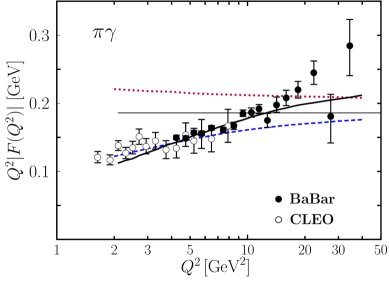
Figure 2: (Color online) The scaled $\pi\gamma$ transition form factor versus $Q^{2}$ evaluated from fit (9) (solid line). The dashed line represents the result presented in [16] which is obtained from the asymptotic distribution amplitude and $\sigma_{\pi}=0.861\,~{}{\rm GeV}^{-1}$. The dotted line is obtained from collinear factorization to NLO accuracy. The thin solid line indicates the asymptotic behavior. Data taken from [2, 20]

3 Confronting with experiment

Now, having specified the details of the MPA, one can analyze the transition form factor by inserting (5) and (2) into (3) and fitting the Gegenbauer coefficients to experiment. From a detailed examination of the data it becomes apparent that besides the transverse size parameter only one Gegenbauer coefficient can safely be determined. If more coefficients are freed the fits become unstable. The coefficients acquire unphysically large absolute values between 1 and 10 and with alternating signs leading to strong compensations among the various terms.

Let us begin with the analysis of the CLEO [20] and BaBar [2] data on the $\pi\gamma$ form factor. A reasonable fit to these data is obtained by taking for the Gegenbauer coefficient $a_{2}^{\pi}$ the face value of a lattice QCD result [21]:

$$a_{2}^{\pi}(\mu_{0})\,=\,0.20$$ (8)

at the scale $\mu_{0}=2\,~{}{\rm GeV}$ (with $\Lambda_{\rm QCD}=0.181\,~{}{\rm GeV}$ and the 1-loop expression for $\alpha_{\rm s}$) and fitting $a_{4}^{\pi}$ and the transverse size parameter, $\sigma_{\pi}$, to the data for $Q^{2}>2.3\,~{}{\rm GeV}^{2}$. The resulting parameters are

$$\sigma_{\pi} = 0.40\pm 0.06\,~{}{\rm GeV}^{-1}\,,$$

$$a_{4}(\mu_{0}) = 0.01\pm 0.06\,,$$ (9)

and $\chi^{2}=34.2$ which appears reasonable given that 28 data points are included in the fit. A fit with just $\sigma_{\pi}$ and $a_{2}^{\pi}$ leads to parameters in agreement with the lattice result (8) and the parameters quoted in (9); the results for the form factor are practically indistinguishable from the first fit. The results for the $\pi\gamma$ form factor of the fit (9) are shown in Fig. 2. At the largest values of $Q^{2}$ the fit seems to be a bit small as compared to the BaBar data. Partially responsible for this fact are the large fluctuations the BaBar data exhibit; the fit compromises between all the data. For comparison the fit presented in [16] which is evaluated from the asymptotic distribution amplitude and $\sigma_{\pi}=0.861\,~{}{\rm GeV}$, is also shown in Fig. 2. This result is obviously too low at large $Q^{2}$, it does not exceed the asymptotic limit of the scaled form factor, $\sqrt{2}f_{\pi}$, in contrast to the BaBar data and the fit (9). Also shown in Fig. 2 is a typical result of the collinear factorization approach to NLO accuracy taking $\mu_{F}=\mu_{R}=Q$ and the Gegenbauer coefficients specified in (8) and (9). Apparently the shape of that result is in conflict with experiment. The difference between this result and the MPA result for the same distribution amplitude reveals the strength of the power corrections taken into account by the MPA. It is to be stressed that, in the collinear factorization approach, a change of the values of the Gegenbauer coefficients or the addition of further coefficients with the proviso that large negative coefficients are excluded, does not alter the shape but only the absolute value of the form factor. Thus, the $\pi\gamma$ transition form factor sets an example of an exclusive observable for which collinear factorization is insufficient for $Q^{2}$ as large as $35\,~{}{\rm GeV}^{2}$.

In Sec. 2 it is mentioned that the Sudakov factor can be viewed as the perturbatively generated transverse part of the wave function. In the the original version of the MPA [18], applied to the electromagnetic form factor of the pion, only this part of the wave function has been taken into account and any intrinsic transverse momentum neglected. With this approximation however, i.e. if the Gaussian in (5) is replaced by 1, a food fit to the form factor data cannot be achieved, the results are too flat as compared to the data and the minimal $\chi^{2}$ is 155. Hence, the ${\bf b}$ dependence of the wave function is an important ingredient of the MPA as has been suggested in [17].

Li and Mishima [15] also applied the MPA to the $\pi\gamma$ transition form factor and achieved a reasonable fit to experiment. In contrast to [1] the flat distribution amplitude, $\Phi_{\pi}\equiv 1$, is used. It is combined with a Gaussian $b$-dependence as in (5) in a kind of wave function. However, this product cannot be considered as a proper wave function in so far as it is not normalizable. It is furthermore argued in [15] that the flat distribution amplitude is accompanied by a threshold factor that represents resummed double logs $\alpha_{\rm s}\ln^{2}{x}$ and $\alpha_{\rm s}\ln^{2}{(1-x)}$ arising from the end-point singularities which occur for the flat distribution amplitude in collinear factorization. The threshold factor combined with the flat distribution amplitude can be viewed as an effective distribution amplitude of the type

$$\Phi_{\pi}^{r}\,=\,\frac{\Gamma(2+2r)}{\Gamma^{2}(1+r)}\,\big{[}x\bar{x}\big{]}^{r}\,.$$ (10)

According to [15], $r$ is about 1 for low $Q^{2}$ and small for $Q^{2}\simeq 35\,~{}{\rm GeV}^{2}$, see Fig. 3. This particular $Q^{2}$-dependence of the power $r$ generates the increase of the form factor required by the BaBar data [2]: At low $Q^{2}$ the effective distribution amplitude is the asymptotic one implying small values of the transition form factor while, at $Q^{2}$ of about $35\,~{}{\rm GeV}^{2}$, the effective distribution amplitude is close to the flat one and hence leads to much larger values of the form factor.

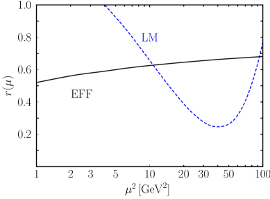
Figure 3: (Color online) The effective power (EFF) of the distribution amplitude (10) compared to the power (LM) of the threshold factor in [15] at the scale $\mu$.

Eq. (10) defines a family of power-like distribution amplitudes. It includes the limiting cases of the asymptotic distribution amplitude for $r=1$ as well as the flat distribution amplitude for $r=0$. Also the square root distribution amplitude proposed in [22] belongs to this family. Expanding (10) upon the Gegenbauer polynomials and using its evolution one can show [19] that, for $0\leq r(\mu_{0})\leq 1$, the distribution amplitude (10) approximately remains power-like under evolution, $r\to r(\mu)$ over a large range of the scale. The power-like distribution amplitude (10) may be examined by fitting the transverse size parameter as well as the power $r(\mu_{0})$ to the data on the $\pi\gamma$ form factor. One finds ($\chi^{2}\,=\,34.4$)

$$\sigma_{\pi} = 0.40\pm 0.05\,~{}{\rm GeV}^{-1}\,,$$

$$r(\mu_{0}) = 0.59\pm 0.06\,.$$ (11)

The quality of this fit to the data on the $\pi\gamma$ form factor is similar to that presented in [15] and to (9). In Fig. 3 the power $r(\mu)$ for the fit (11) is compared to the scale dependence of the threshold factor used in [15] (in this work the power is set to unity for $\mu^{2}\raisebox{-4.0pt}{$\,\stackrel{{\scriptstyle\textstyle<}}{{\sim}}\,$}4\,~{}{\rm GeV}^{2}$). As can be seen from Fig. 3 the distribution amplitude (10) exhibits the usual evolution behavior, it monotonically evolves into the asymptotic one, $\Phi_{\rm AS}$, for $\mu\to\infty$. On the other hand, the scale dependence of the threshold factor or the effective distribution amplitude advocated for in [15], is drastically different.

Let us now turn to the analysis of the $\eta\gamma$ and $\eta^{\prime}\gamma$ form factors. They can be expressed as a sum of the flavor-octet and flavor-singlet contributions [7]

$$F_{P\gamma}\,=\,F^{8}_{P\gamma}+F^{1}_{P\gamma}\,.$$ (12)

As is the case for the $\pi\gamma$ form factor the functions $F^{i}_{P\gamma}$ ($i=1,8$) are proportional to the constants $f_{P}^{i}$ assigned to the decays of meson $P$ through the SU(3)_F octet or singlet axial-vector weak currents which are defined by the matrix elements

$$\langle 0\mid J_{\mu 5}^{i}\mid P(p)\rangle\,=\,if_{P}^{i}\,p_{\mu}\,.$$ (13)

Adopting the general parameterization [23]

$$f_{\eta}^{8} = f_{8}\cos{\theta_{8}}\,,\qquad f_{\eta}^{1}\,=\,-f_{1}\sin{\theta_{1}}\,,$$

$$f_{\eta^{\prime}}^{8} = f_{8}\sin{\theta_{8}}\,,\qquad f_{\eta^{\prime}}^{1}\,=\,\phantom{-}f_{1}\cos{\theta_{1}}\,,$$ (14)

one can show [24] that on exploiting the divergences of the axial-vector currents - which embody the axial-vector anomaly - the mixing angles, $\theta_{8}$ and $\theta_{1}$, differ considerably from each other and from the state mixing angle, $\theta$. In [24] the mixing parameters have been determined:

$$f_{8} = 1.26\,f_{\pi}\,,\qquad f_{1}\,=\,1.17\,f_{\pi}\,,$$

$$\theta_{8} = -21.2^{\circ}\,,\qquad\theta_{1}\,=\,-9.2^{\circ}\,.$$ (15)

Assuming particle-independent [7, 24] wave functions, $\Psi^{8}$ and $\Psi^{1}$, for the valence Fock states of the respective octet and singlet $\eta$ mesons and parameterizing them as in (5) with decay constants $f_{8}$ and $f_{1}$ instead of $f_{\pi}$, one can cast the transition form factors into the form

$$F_{\eta\gamma} = \cos{\theta_{8}}\,F^{8}-\sin{\theta_{1}}\,F^{1}$$

$$F_{\eta^{\prime}\gamma} = \sin{\theta_{8}}\,F^{8}+\cos{\theta_{1}}\,F^{1}\,.$$ (16)

The charge factors in (4) read (with $P=1,8$)

$$C_{8} = (e_{u}^{2}+e_{d}^{2}-2e_{s}^{2})/\sqrt{6}\,,$$

$$C_{1} = (e_{u}^{2}+e_{d}^{2}+e_{s}^{2})/\sqrt{3}\,.$$ (17)

The asymptotic behavior of the form factors is

$$Q^{2}F^{8}\to\sqrt{\frac{2}{3}}f_{8}\,,\qquad Q^{2}F^{1}\to\frac{4}{\sqrt{3}}f_{1}\,.$$ (18)

The renormalization-scale dependence of the singlet-decay constant [23] is omitted since the anomalous dimension controlling it is of order $\alpha_{\rm s}^{2}$ and, hence, leads to tiny effects.

For the singlet $\eta$ meson, $\eta_{1}$, there is also a glue-glue Fock component which, however, only contributes to NLO (or higher) of the hard scattering [26, 27, 28]. In the MPA analysis the glue-glue Fock component does not contribute directly but only through the matrix of the anomalous dimensions and the mixing of the singlet quark-antiquark with the glue-glue distribution amplitude. It is assumed in [1] that the Gegenbauer coefficients of the glue-glue distribution amplitude are zero at a low scale of order $1\,~{}{\rm GeV}$. Hence, the quark-antiquark singlet distribution amplitude practically evolves with the same anomalous dimensions as the octet distribution amplitude.

The two form factors $F^{8}$ and $F^{1}$ can now be evaluated from (3) and (4) in full analogy to the $\pi\gamma$ transition form factor. The data on $F^{8}$ and $F^{1}$ are extracted from the CLEO [20] and BaBar [4] data using (16). As for the $\pi\gamma$ form factor only the transverse size parameter and one Gegenbauer coefficient for each wave function can be determined. The best fit is obtained with the parameters:

$$\sigma_{8} = 0.84\pm 0.14\,~{}{\rm GeV}^{-1}\,,$$

$$a_{2}^{8}(\mu_{0}) = -0.06\pm 0.06\,,$$

$$\sigma_{1} = 0.74\pm 0.05\,~{}{\rm GeV}^{-1}\,,$$

$$a_{2}^{1}(\mu_{0}) = -0.07\pm 0.04\,.$$ (19)

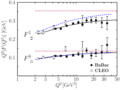
Figure 4: (Color online) The octet and singlet form factors. Dotted lines represent the asymptotic behavior (18), the dashed lines the results obtained in [7]. The solid lines represent the new fit (19). Data taken from [20, 4]

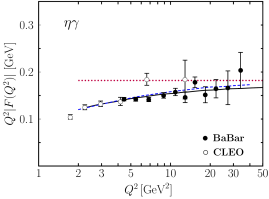
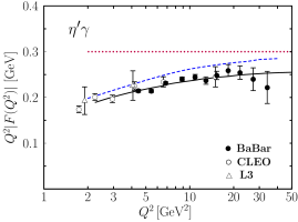
Figure 5: (Color online) The scaled $\eta\gamma$ (left) and $\eta^{\prime}\gamma$ (right) transition form factor versus $Q^{2}$. Data taken from [20, 25, 4]. For notations refer to Fig. 4

The values of $\chi^{2}$ are 15.0 and 14.1 for the octet and singlet cases, respectively (for 16 data points in each case). In Fig. 4 the results of this fit are compared to the data on $F^{8}$ and $F^{1}$. The quality of this fit is very good. In contrast to the $\pi\gamma$ case the data on both $F^{8}$ and $F^{1}$ lie below the asymptotic results (18). The combination of these two form factors into the physical ones according to (16) leads to the results shown in Fig. 5. Again very good agreement with the data is to be observed. Also shown in Figs. 4 and 5 are the results obtained in [7] which have been evaluated from the asymptotic distribution amplitudes (with $\sigma_{1}=\sigma_{8}=0.861\,~{}{\rm GeV}^{-1}$). The octet as well as the $\eta\gamma$ form factors of [7] are in very good agreement with experiment while the results for $F^{1}$ and the $\eta^{\prime}\gamma$ form factor are somewhat too large.

Since the octet and singlet wave functions in (19) are very close to the asymptotic one, the power corrections generated by the MPA are small. Therefore, and in sharp contrast to the $\pi\gamma$ case, an analysis of the $\eta\gamma$ and $\eta^{\prime}\gamma$ form factors within the collinear factorization approach is also possible. In this case information on the glue-glue Fock component of the $\eta_{1}$ may be extracted [28]. Even with form factor data up to about $35\,~{}{\rm GeV}^{2}$ it is apparently not possible to discriminate between logarithmic and power corrections.

The analysis of the $\eta\gamma$ and $\eta^{\prime}\gamma$ form factors performed in [1] relies on the mixing parameters (15) determined in [24, 29]. Mixing of the $\eta$ and $\eta^{\prime}$ mesons has been frequently investigated. Although in most cases not the same set of processes as in [24, 29] has been analyzed the mixing parameters found are in reasonable agreement with (15) within occasionally large errors (see the discussion in [30]). An exception is [31] where the parameters markedly differ from (15). However, as pointed out in [32], the parameters quoted in [31] are in conflict with the transition form factors.

The treatment of the $\eta_{c}\gamma$, also measured by the BaBar collaboration [3], differs from that of the three other cases. There is a second large scale in addition to the virtuality of one of the photons, namely the mass of the $\eta_{c}$ ($M_{\eta_{c}}$) or that of the charm quark ($m_{c}$). It cannot be neglected in a perturbative calculation in contrast to the case of the light mesons where quark and hadron masses do not play a role. Despite this the $\eta_{c}\gamma$ form factor is to be calculated from (3) but the hard scattering amplitude to lowest order perturbative QCD reads [8]

$$T_{H}\,=\,\frac{4\sqrt{6}\,e_{c}^{2}}{xQ^{2}+(1+4x(1-x))m_{c}^{2}+{\bf k}_{\perp}^{2}}\,.$$ (20)

The symmetry of the problem under the replacement of $x$ by $1-x$ is already taken into account in (20). Due to the involved second large scale in the problem the $\eta_{c}\gamma$ form factor can be calculated even at $Q^{2}=0$.

The light-cone wave function of the $\eta_{c}$ is parameterized as in (5). Following [8, 33] the distribution amplitude is chosen as

$$\Phi_{\eta_{c}}\,=\,N(\sigma_{\eta_{c}})x\bar{x}\exp{\Big{[}-\sigma^{2}_{\eta_{c}}M_{\eta_{c}}^{2}\frac{(x-1/2)^{2}}{x\bar{x}}\Big{]}}$$ (21)

where $N(\sigma_{\eta_{c}})$ is determined from the usual requirement $\int_{0}^{1}dx\Phi_{\eta_{c}}(x)=1$. The distribution amplitude exhibits a pronounced maximum at $x=1/2$ and is exponentially damped in the end-point regions. It describes an essentially non-relativistic $c\bar{c}$ bound state; quark and antiquark approximately share the meson’s momentum equally. In the hard scattering amplitude the charm quark mass occurs while in the distribution amplitude the meson mass is used. This property of the latter distribution amplitude is a model assumption which contributes to the theoretical uncertainty of the results. In the sense of the non-relativistic QCD [34] $2m_{c}$ and $M_{\eta_{c}}$ are equivalent. In (3) the Sudakov factor can be set to 1 in the case at hand since it is mainly active in the end-point regions (see the discussion in Sect. 2) which are already strongly damped by the $\eta_{c}$ wave function. Even the ${\bf k}_{\perp}$ dependence of the hard scattering amplitude plays a minor role. The evolution behavior of the $\eta_{c}$ distribution amplitude is unknown in the range where $Q^{2}$ is of order of $M_{\eta_{c}}^{2}$ and is therefore ignored here. Consequently, also the running of the charm quark mass is omitted.

The normalization of the $\eta_{c}\gamma$ transition form factor is fixed by its value at $Q^{2}=0$ which is related to two-photon decay width. However, this decay width is experimentally not well known [35]. It is therefore advisable to normalize the form factor by its value at $Q^{2}=0$ all the more so since the recent BaBar data [3] are also presented this way. Doing so the perturbative QCD corrections at $Q^{2}=0$ to the $\eta_{c}\gamma$ transition form factor which are known to be large [36], are automatically included. Also the $\alpha_{\rm s}$ corrections for $Q^{2}\raisebox{-4.0pt}{$\,\stackrel{{\scriptstyle\textstyle<}}{{\sim}}\,$}M_{\eta_{c}}^{2}$ [26] cancel to a high degree in the ratio $F_{\eta_{c}\gamma}(Q^{2})/F_{\eta_{c}\gamma}(0)$. Even at $Q^{2}=10\,~{}{\rm GeV}^{2}$ their effect is less than $5\%$, see the discussion in [8]. The uncertainties in the present knowledge of the $\eta_{c}$ decay constant do also not enter the predictions for this ratio.

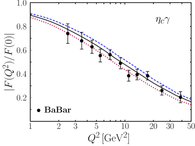
Figure 6: (Color online) The $\eta_{c}\gamma$ form factor scaled by its value at $Q^{2}=0$. Data taken from [3]. The solid (dotted) line represents the results of a calculation with the values of the parameters quoted in (22) (with $m_{c}=1.26\,~{}{\rm GeV}$). The dashed line is the prediction given in [8]

The recent Babar data on the $\eta_{c}\gamma$ form factor [3] are shown in Fig. 6. The predictions given in [8] which have been evaluated from $m_{c}=M_{\eta_{c}}/2$, are about one standard deviation too large but with regard to the uncertainties of the theoretical calculation, as for instance the exact value of the mass of the charm quark, one can claim agreement between theory and experiment. A little readjustment of the value of the charm quark mass improves the fit. Thus, with the parameters

$$m_{c}\,=\,1.35\,~{}{\rm GeV},\qquad\sigma_{\eta_{c}}\,=\,0.44\,~{}{\rm GeV}^{-1}\,,$$ (22)

a perfect agreement with experiment is achieved as is to be seen in Fig. 6. For comparison there are also shown results evaluated from $m_{c}=1.21\,~{}{\rm GeV}$.

The form factors scaled by their respective asymptotic behaviors are displayed in Fig. 7 for a large range of $Q^{2}$. Asymptotically they all tend to 1. The $\pi\gamma$ form factor approaches 1 from above, the other ones from below. The approach to 1 is a very slow process; even at $500\,~{}{\rm GeV}^{2}$ the limiting behavior has not yet been reached. It is also evident from Fig. 7 that, forced by the BaBar data, there are strong violations of SU(3)_F flavor symmetry in the ground state octet of the pseudoscalar mesons at large $Q^{2}$. In other processes involving pseudoscalar mesons, e.g. two-photon annihilations into pairs of pseudoscalar mesons [37, 38], such large flavor symmetry violations have not been observed. Below $8\,~{}{\rm GeV}^{2}$, i.e. in the range of the CLEO data, flavor symmetry breaking is much milder. The $\eta_{c}\gamma$ transition form factor which is also shown in Fig. 7, behaves different - the large charm-quark mass slows down the approach to the asymptotic limit

$$Q^{2}F_{\eta_{c}\gamma}\to\frac{8f_{\eta_{c}}}{3}\,.$$ (23)

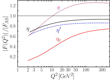
Figure 7: (Color online) The $P-\gamma$ transition form factors scaled by the corresponding asymptotic behavior, versus $Q^{2}$. The thick solid (dashed, dotted, thin solid) line represents the case of the $\eta$ ($\eta^{\prime}$, $\pi$, $\eta_{c}$) meson. Parameters are taken from fit (9), (19) and (22)

4 Summary

In this talk it is reported on an analysis of the form factors for the transitions from a photon to a pseudoscalar meson [1]. The analysis is performed within the MPA which bases on ${\bf k}_{\perp}$ factorization. In combination with the hard scattering kernel the Sudakov suppressions which are an important ingredient of the MPA and which represents radiative corrections in next-to-leading-log approximation summed to all orders of perturbation theory, lead to a series of power suppressed terms which are accumulated in the soft regions. Since these corrections grow with the Gegenbauer index the transition form factors are only affected by the few lowest Gegenbauer terms of the distribution amplitude, the higher ones do practically not contribute. How many Gegenbauer terms are relevant depends on the range of $Q^{2}$ considered: In the $Q^{2}$ range covered by the CLEO data [20] ($<10\,~{}{\rm GeV}^{2}$) it suffices to use just the asymptotic distribution amplitude in order to fit the CLEO data. With the BaBar data [2, 4] at disposal, covering the unprecedented large range $4\,~{}{\rm GeV}^{2}<Q^{2}<35\,~{}{\rm GeV}^{2}$, the next or the next two Gegenbauer terms have to be taken into account or, turning the argument around, can be determined from an analysis of the data on the transition form factors. Indeed this is what has been done in [1]. From this analysis it turned out that for the case of the pion a fairly strong contribution from $a_{2}$ is required by the data while for the $\eta$ and $\eta^{\prime}$ much smaller deviations from the asymptotic distribution amplitude are needed. For these cases the results from a previous calculation within the MPA [7] are already in fair agreement with the BaBar data, nearly perfect for the $\eta$, slightly worse for the $\eta^{\prime}$. Comparing the $\pi\gamma$ form factor with the $\eta\gamma$ or more precisely the $\eta_{8}\gamma$ one, one observes a strong breaking of flavor symmetry in the ground-state octet of the pseudoscalar mesons. In other processes involving pseudoscalar mesons such large flavor symmetry violations have not been observed. With regard to the theoretical importance of the transition form factors, in particular the role of collinear factorization a remeasurement, e.g. by the BELLE collaboration, would be highly welcome.

Acknowledgements It is a pleasure to thank Stanislav Dubnicka and Suzanna Dubnickova for the kind invitation to the conference on Hadron Structure held in Tatranska Strba (Slovakia) and for the hospitality extended to the authors. This work is supported in part by the BMBF, contract number 06RY258.

References

- [1] P. Kroll, Eur. Phys. J. C71, 1623 (2011).
- [2] B. Aubert et al. [The BABAR Collaboration], Phys. Rev. D 80, 052002 (2009).
- [3] J. P. Lees et al. [The BABAR Collaboration], Phys. Rev. D 81 (2010) 052010.
- [4] V. P. Druzhinin et al. [BABAR Collaboration], arXiv:1101.1142 [hep-ex].
- [5] G. P. Lepage and S. J. Brodsky, Phys. Lett. B 87, 359 (1979).
- [6] F. del Aguila and M. K. Chase, Nucl. Phys. B 193, 517 (1981); E. Braaten, Phys. Rev. D 28, 524 (1983).
- [7] T. Feldmann and P. Kroll, Eur. Phys. J. C 5, 327 (1998).
- [8] T. Feldmann and P. Kroll, Phys. Lett. B 413, 410 (1997).
- [9] A.V. Radyushkin, Phys. Rev. D 80, 094009 (2009).
- [10] M. V. Polyakov, JETP Lett. 90, 228 (2009).
- [11] S. S. Agaev, V. M. Braun, N. Offen and F. A. Porkert, Phys. Rev. D83, 054020 (2011).
- [12] A. P. Bakulev, S. V. Mikhailov and N. G. Stefanis, Acta Phys. Polon. Supp. 3, 943 (2010).
- [13] A. E. Dorokhov, arXiv:1003.4693 [hep-ph].
- [14] J. Botts and G. Sterman, Nucl. Phys. B 325, 62 (1989).
- [15] H.-S. Li and S. Mishima, Phys. Rev. D 80, 074024 (2009).
- [16] P. Kroll and M. Raulfs, Phys. Lett. B 387, 848 (1996).
- [17] R. Jakob and P. Kroll, Phys. Lett. B 315, 463 (1993) [Erratum-ibid. B 319, 545 (1993)].
- [18] H. n. Li and G. Sterman, Nucl. Phys. B 381, 129 (1992).
- [19] V. Braun, M. Diehl and P. Kroll, work in progress.
- [20] J. Gronberg et al. [CLEO Collaboration], Phys. Rev. D 57, 33 (1998).
- [21] V.M. Braun et al [QCDSF/UKQCD collaboration], Phys. Rev. D 74, 074501 (2006).
- [22] S. J. Brodsky and G. F. de Teramond, Phys. Rev. D 77, 056007 (2008).
- [23] H. Leutwyler, Nucl. Phys. Proc. Suppl. 64 (1998) 223. R. Kaiser and H. Leutwyler, arXiv:hep-ph/9806336;
- [24] T. Feldmann, P. Kroll and B. Stech, Phys. Rev. D 58, 114006 (1998).
- [25] M. Acciarri et al. [L3 Collaboration], Phys. Lett. B 418, 399 (1998).
- [26] M. A. Shifman and M. I. Vysotsky, Nucl. Phys. B186, 475 (1981).
- [27] V. N. Baier and A. G. Grozin, Nucl. Phys. B192, 476 (1981).
- [28] P. Kroll and K. Passek-Kumericki, Phys. Rev. D 67, 054017 (2003).
- [29] T. Feldmann, P. Kroll, B. Stech, Phys. Lett. B449, 339-346 (1999).
- [30] P. Kroll, Mod. Phys. Lett. A20, 2667-2684 (2005).
- [31] R. Escribano, J. -M. Frere, JHEP 0506, 029 (2005).
- [32] Y. N. Klopot, A. G. Oganesian, O. V. Teryaev, [arXiv:1106.3855 [hep-ph]].
- [33] M. Wirbel, B. Stech and M. Bauer, Z. Phys. C 29, 637 (1985).
- [34] G. T. Bodwin, E. Braaten and G. P. Lepage, Phys. Rev. D 51, 1125 (1995) [Erratum-ibid. D 55, 5853 (1997)].
- [35] K. Nakamura et al. [Particle Data Group], JPG 37, 075021 (2010).
- [36] R. Barbieri, E. d’Emilio, G. Curci, E. Remiddi, Nucl. Phys. B154, 535 (1979).
- [37] M. Diehl and P. Kroll, Phys. Lett. B 683, 165 (2010).
- [38] S. Uehara et al. [Belle Collaboration], Phys. Rev. D 80, 032001 (2009).