Qubit state detection using the quantum Duffing oscillator

Abstract

We introduce a detection scheme for the state of a qubit, which is based on resonant few-photon transitions in a driven nonlinear resonator. The latter is parametrically coupled to the qubit and is used as its detector. Close to the fundamental resonator frequency, the nonlinear resonator shows sharp resonant few-photon transitions. Depending on the qubit state, these few-photon resonances are shifted to different driving frequencies. We show that this detection scheme offers the advantage of small back action, a large discrimination power with an enhanced read-out fidelity, and a sufficiently large measurement efficiency. A realization of this scheme in the form of a persistent current qubit inductively coupled to a driven SQUID detector in its nonlinear regime is discussed.

I Introduction

The efficient and reliable detection of the quantum mechanical state of a nanoscale system is a key component of all present designs of quantum circuits.Clerk10 One nondestructive readout scheme currently in use for the important class of superconducting flux qubits is based on a heterodyne detection of the dynamic response of a dc superconducting quantum interference device (dc-SQUID) detector which is inductively coupled to the qubit. Lupascu04 ; Lupascu05 Thereby, the dc-SQUID is operated in its linear regime as a shunted variable inductor in a resonant circuit. In this set-up, its resonance frequency depends on the magnetic flux generated by the qubit being in the ground or excited state. Hence, measuring the impedance of the resonant circuit as a function of an externally applied bias current yields two characteristic Lorentzian resonances at two different resonance frequencies, which depend on the two qubit states. This detection scheme, hence, allows us to infer the state of the qubit from the resonant response of the detector in the nanocircuit. In order that a reliable discrimination of the two qubit states becomes possible in this continuous type of readout design, the probability distributions for the readout values have to be only weakly overlapping. Due to thermal and quantum fluctuations, the readout naturally is a random process,Lupascu05 and the noise properties of the nanocircuit around the detector resonances determine the discrimination power of the set-up.

An alternative readout scheme is the Josephson bifurcation amplifier.Siddiqi04 ; Vijay09 It is based on a classical driven nonlinear resonator and exploits the classical bifurcation point of the dynamically induced bistability with a small- and a large-oscillation state.Nayfeh79 The response (or output) of the nonlinear resonator around the bifurcation point is very sensitive to small changes in the circuit parameters. This is an ideal prerequisite for a sensitive detector. Depending on the state of the qubit to be sensed, the resonator bifurcation point is shifted to a different frequency, allowing for large discrimination powers between the large- and small-oscillation detector state of up to $98\%$.Lupascu06 Nevertheless, since the detector is a classical macroscopic device, it introduces considerable dephasing and relaxation to the qubit state, yielding a reduced contrast of the qubit Rabi oscillations of less than $90\%$.Lupascu06 This implies that the thermal noise properties of the nonlinear detector (together with semiclassical corrections due to quantum fluctuations) around the classical bifurcation point determine the discrimination power between the two states close to the classical bifurcation point. Dykman79 ; Dykman90 ; Dmitriev86 ; Dykman88 Hence, it would be desirable to combine the advantage of a large discrimination power of a nonlinear detector with the reduced noise sensitivity of a nanocircuit operated close to the quantum regime.

In this paper, we introduce a combination of both strategies and propose a nonlinear detector scheme in the form of a nonlinear resonator with an amplitude modulated drive in its few-photon deep quantum regime. In particular, in this regime, we shall exploit sharp multiphoton resonances in the nonlinear resonator, Peano04 ; Peano06a ; Peano06b which are induced by the external driving field close to the fundamental resonator frequency. They can be used for the detection of the states of the qubit and offer the advantage of being rather sharp and externally tunable by varying the parameters of the external drive. The concept is an extension of the case of a linear resonator, where the fundamental resonance frequency is shifted depending on the qubit state. However, the multiphoton resonances in the nonlinear detector close to the detector’s fundamental frequency show very small line widths. The width of the $N$-photon resonance is determined by the corresponding $N$-photon Rabi frequency, which decreases with increasing photon number. The sharp resonance lines, in turn, offer the advantage that only a few measurement cycles are necessary to ensure a large discrimination power. To understand the back action of the nonlinear multiphoton detector on the qubit state, we determine the relaxation rate of the qubit due to the coupling to the driven dissipative nonlinear oscillator around a multiphoton resonance. Notably, the back action of the resonator on the qubit is sufficiently weak, yielding to a good qubit-state measurement fidelity. Furthermore, we show that the discrimination power of the set-up is rather large and beyond $98\%$ for our choice of realistic parameters of a flux qubit circuit. In fact, it gives rise to an enhanced measurement fidelity as compared to the linear parametric oscillator. Furthermore, we show that the nonlinear multiphoton detector does not have a worse measurement efficiency as compared to the linear detector scheme. We determine the measurement efficiency of the set-up via the ratio of the time it takes to collect enough information on the qubit state (measurement time) and the relaxation time. It turns out that the measurement efficiency does not considerably decrease as compared to the linear case. Hence, the detection scheme indeed has the advantage of an overall reduced back action in combination with an enhanced discrimination power, together with a sufficiently large measurement efficiency.

An experimental realization of a driven nonlinear resonator in its few-photon quantum regime is in principle possible with present set-ups and technology. In a recent experiment,Murch10 a nanoscale superconducting microwave resonator has been driven to its nonlinear regime by fast frequency-chirped voltage pulses. At low enough temperature, the regime of quantum noise has been reached. In this experiment, the applied driving strength has been rather large, which corresponds to a large photon number transferred to the resonator. No particular few-photon resonances have been revealed and the nonlinear response is similar to previous schemes on classical bifurcation detectors using a time-dependent driving frequency.Naaman08 . However, the route to the few-photon regime seems to be clear.

The paper is organized as follows. In Sec. II, we start from a typical experimental setup for the flux qubit and its SQUID detector and we derive the Hamiltonian model. This serves to motivate an experimental realization of our proposed detection scheme. Moreover, we discuss the regime of validity of the model. In accordance with the approximation made in Sec. II, we continue the study of the coherent dynamics in Sec. III in the rotating wave approximation. Dissipative coupling to the environment is included on the level of a Born-Markov master equation in the rotating frame in Sec. IV. In Sec. V, we analyze the multiphoton transitions in the nonlinear response of the Duffing oscillator and show that their resonance frequency depends on the qubit state. Then, in Sec. VI we determine the back action of the driven dissipative detector on the qubit dynamics by analyzing the population difference of the qubit states at the multiphoton transitions in the detector. Furthermore, we determine the measurement efficiency in Sec. VII.

II Model

In order to relate the theoretical approach in the following to realistic devices, we start by deriving the model from standard set-ups already realized in experiments. For this, we use a typical architecture of a persistent current qubit which is inductively coupled to a driven SQUID.

II.1 Persistent current qubit

We consider the experimental set-up used in Ref. flux-qubit, for the qubit, consisting of a superconducting loop interrupted by three Josephson junctions, two of which have equal Josephson energies, while the coupling energy of the third is smaller, in order to yield a double-well potential configuration. In this low-inductance circuit, the flux through the loop remains close to the externally applied value $\Phi_{\rm qb}$. When the latter is close to $(n+1/2)\Phi_{0}$, where $n$ is an integer and $\Phi_{0}$ is the flux quantum, the device is described by the Hamiltonian in terms of the Pauli matrices $\sigma_{x,z}$ as ($\hbar=1$)

$$H_{\rm qb}=\frac{\epsilon}{2}\,\sigma_{z}-\frac{\Delta}{2}\,\sigma_{x},$$ (1)

with the two eigenstates $|\!\!\uparrow\rangle$ and $|\!\!\downarrow\rangle$ of $\sigma_{z}$ corresponding to the two persistent current states $\pm I_{p}$. The minimal energy level splitting $\Delta$ and the current $I_{p}$ are determined by the charging and Josephson energies of the Josephson junctions. The asymmetry is given by $\epsilon=2I_{p}(\Phi_{\rm qb}-\Phi_{\rm 0}/2)$. In the energy eigenbasis, the Hamiltonian follows as $H_{\rm qb}=\omega_{\rm qb}\tau_{z}/2$, with $\omega_{\rm qb}=\sqrt{\epsilon^{2}+\Delta^{2}}$, and $\tau_{z}=\sigma_{z}\cos\theta-\sigma_{x}\sin\theta$ is the corresponding Pauli matrix with $\tan\theta=\Delta/\epsilon$. The detection of the qubit state essentially involves the measurement of the magnetic flux produced by the persistent current states. To this end, one can use the driven SQUID as a sensitive magnetometer, Lupascu04 operating in its nonlinear region. Below, we will restrict to the few-photon deep quantum regime.

II.2 Driven SQUID as a nonlinear quantum detector

We consider the standard setup of a dc-SQUID formed by two Josephson junctions in a superconducting loop, but subject to a time-dependent external bias current.Vijay09 Moreover, we assume a negligible ring inductance $L_{R}$ of the SQUID (low-inductance approximation). Soerensen76 In this configuration, the superconducting phase differences at each junction, $\chi_{1}$ and $\chi_{2}$, play the role of dynamical variables with a constraint given by the flux quantization, i.e., $\chi_{1}-\chi_{2}=-\Phi_{\rm sq}/\varphi_{0}\equiv-2\pi\varphi_{\rm ex}$, where $\Phi_{\rm sq}$ is the external magnetic flux piercing the superconducting loop and $\varphi_{0}=\Phi_{0}/2\pi$. Note that within the low-inductance approximation, $L_{R}I_{\rm 0c}\ll\varphi_{0}$ with the critical current $I_{\rm 0c}$ of the SQUID. Thus, the system is described by the generalized coordinate $\chi_{+}=(\chi_{1}+\chi_{2})/2$, with the effective Lagrangian Clarke01

$$L_{\rm sq}(\chi_{+},\dot{\chi}_{+},t) = \varphi_{0}^{2}\,C_{0}\,\dot{\chi}_{+}^{2}+E_{J}\cos\left(\pi\varphi_{\rm ex}\right)\cos(\chi_{+})$$ (2)

$$-\varphi_{0}I_{\rm b}(t)\,\chi_{+},$$

where we have assumed a symmetric loop, with $E_{J}=\varphi_{0}I_{\rm 0c}$ as the Josephson energy, and $C_{0}$ as the capacitance of each junction. Moreover, we include a time-periodic ac current $I_{\rm b}(t)=I_{0}\cos(\omega_{\rm ex}t)$ with frequency $\omega_{\rm ex}$ and amplitude $I_{0}$ injected “into” the loop. The above Lagrangian describes an effective superconducting loop (with a negligible ring inductance) with a single Josephson junction Lupascu05 with a tunable Josephson energy $E_{J}\cos(\pi\varphi_{\rm ex})$, critical current $I_{\rm c}=2I_{\rm 0c}|\cos\pi\varphi_{\rm ex}|$, cross-junction phase difference $\chi_{+}$, and capacitance $C=2C_{0}$. In order to tune the resonance frequency, the SQUID is shunted Vijay09 with a capacitance $C_{s}\gg C$. Next, we shall establish the optimal working point of the qubit-detector system, where the dissipative influence entering via the detector is minimal.

II.2.1 Qubit-detector interaction

The qubit and the SQUID are coupled by means of their mutual inductance $M$.Lupascu05 ; Makhlin01 Thereby, the SQUID induces the flux $MI_{\circlearrowleft}$ in the qubit loop, where $I_{\circlearrowleft}$ is the circulating current in the SQUID. The latter can be determined by using current conservation in the loop and the Josephson relations for the two junctions in the SQUID. For the symmetric SQUID,Lupascu05 it follows that $I_{\circlearrowleft}(t)=I_{\rm c0}\sin(\pi\varphi_{\rm ex})\cos(\chi_{+}(t))$. Thus, the total magnetic flux in the qubit is affected by its coupling with the SQUID, and it is composed of the external flux and the SQUID-generated contribution, i.e., $\Phi_{\rm qb}\rightarrow\Phi_{\rm qb}+MI_{\circlearrowleft}(t)$. This implies that the energy bias of the qubit acquires a contribution that depends on the circulating current in the SQUID, leading to the effective asymmetry $\epsilon_{f}=\epsilon(\Phi_{\rm qb})+\beta(I_{\circlearrowleft}(t))$, where $\beta(I_{\circlearrowleft}(t))=2MI_{p}I_{\circlearrowleft}(t)$.

Therefore, two sources of noise can affect the qubit dynamics, i.e., the fluctuations from the external flux $\Phi_{\rm qb}$ and from the bias current $I_{\rm b}(t)$ in the SQUID,Bertet05 which is related to $\chi_{+}$ by the Josephson equation $I_{b}(t)=I_{c0}\sin(\chi_{+}(t))$. By tuning the bias current to the critical value $I^{*}_{\rm b}$ characterized by $(d\beta/dI_{\rm b})_{I_{\rm b}=I^{*}_{\rm b}}=0$, the influence from current fluctuations in the SQUID can be minimized Bertet05 and the optimal working point is reached. For a nonsymmetric SQUID, the lowest-order contribution is linear in $I_{b}$,Clarke01 ; Bertet05 while in the symmetric case this lowest-order contribution vanishes, which implies that around the optimal working point the phase $\chi_{+}$ is very small, $\chi_{+}\sim 0$. In the following, we consider a setup close to the optimal point, where we can expand the expression for $I_{\circlearrowleft}$ up to second order in $\chi_{+}$, yielding the interaction term

$$H_{\rm qb-sq}=\tilde{g}\chi_{+}^{2}\hat{\sigma}_{z},$$ (3)

with the coupling constant $\tilde{g}=2I_{p}I_{\rm 0c}M\sin(\pi\varphi_{\rm ex})$.

II.2.2 SQUID modelled as a Duffing oscillator

As we operate the detector in its nonlinear regime, we expand the potential term $V(\chi_{+})=-E_{J}\cos\left(\pi\varphi_{\rm ex}\right)\cos(\chi_{+})\simeq V_{0}+m\Omega^{2}\chi_{+}^{2}/2-\tilde{\alpha}\chi_{+}^{4}$ in Eq. (2) around the optimal point up to fourth order in $\chi_{+}$, where $m=\varphi_{0}^{2}C_{\rm s}$ is the effective mass, $\Omega=\left(I_{\rm c}/\varphi_{0}C_{\rm s}\right)^{1/2}$ the corresponding frequency, and $\tilde{\alpha}=m\Omega^{2}/4$ the strength of the nonlinearity. We switch to a description in terms of the creation and annihilation operators $a$ and $a^{\dagger}$, defined by $\chi_{+}=\chi_{0}(a+a^{\dagger})$ with $\chi_{0}=\sqrt{1/(2m\Omega)}$ the zero-point energy of the phase $\chi_{+}$. Adding the time-dependent driving term yields us to the Hamiltonian of the driven SQUID described by the quantum Duffing oscillator model

$$H_{\rm sq}=\Omega\,a^{\dagger}a-\frac{\alpha}{12}(a+a^{\dagger})^{4}+f(a+a^{\dagger})\cos\left(\omega_{\rm ex}t\right),$$ (4)

with nonlinearity and driving strength given by $\alpha=3I_{c}\varphi_{0}\chi_{0}^{4}$, and $f=I_{0}\varphi_{0}\chi_{0}$, respectively. Similarly, the interaction Hamiltonian in terms of ladder operators reads as

$$H_{\rm qb-sq}=\frac{g}{2}(a+a^{\dagger})^{2}\sigma_{z},$$ (5)

with $g=2\tilde{g}\chi_{0}^{2}$.

Notice that $g$ and $\alpha$ depend on the external flux $\varphi_{\rm ex}$, i.e., they are tunable in a limited regime with respect to the desired oscillator frequency $\Omega$, where the coupling term is considered as a perturbation to the SQUID ($g<\alpha$), in order to keep the dynamics of the oscillator to dominate. The dependence of the dimensionless ratios $\alpha/\Omega$ and $g/\Omega$ is shown in Fig. 1.

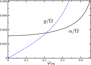
Figure 1: (Color online) Dependence of the dimensionless ratios $\alpha/\Omega$ and $g/\Omega$ on the external flux $\varphi_{\rm ex}$ in the SQUID. The parameters of the SQUID are chosen as $C_{s}=7.65$ pF, $I_{c0}=200$ nA, $I_{p}=300$ nA, and $M=40$ pH. Lupascu05

We restrict to parameters of the external magnetic flux in the SQUID loop, which generate a weak nonlinearity and a weak qubit-detector coupling strength, $\{\alpha,g\}\ll\Omega$, i.e., for $\varphi_{\rm ex}\sim 0$. A typical dependence of both parameters for typical experimental parameters is shown in Fig. 1. Both cases of $g/\Omega>\alpha/\Omega$ and $g/\Omega<\alpha/\Omega$ can be achieved. For our purpose of a qubit-detector setup, the qubit-resonator coupling typically will be required as small enough in order to ensure a minimal back action. On the other hand, the qubit-detector coupling should be large enough so that an efficient detection of the qubit state becomes possible. As is shown in Fig. 1 and will be quantitatively discussed in the sequel of this paper, this can indeed be achieved for realistic parameters. Moreover, the choice of the parameter regime also justifies us to restrict the influence of the resonator coupling on the effective qubit bias to lowest order in $\chi_{+}$ only. Eventually, the total system is described by the Hamiltonian $H(t)=H_{\rm qb}+H_{\rm qb-sq}+H_{\rm sq}(t)$.

III Coherent dynamics and rotating-wave approximation

Before we address the dynamics of the detection scheme based on the nonlinear response of the Duffing oscillator to the applied periodic driving in the stationary regime, we discuss the coherent dynamics generated by $H(t)$, which is periodic in time.

Here, we are interested in exploiting few-photon transitions in the detector around the fundamental detector frequency $\Omega$. Hence, higher harmonics have a small amplitude and can effectively be neglected. Furthermore, we focus on the regime of weak nonlinearity, weak driving, and weak qubit-detector coupling as characterized by $\{\alpha,f,g\}\ll\Omega$. The proposed mechanism of detection is most conveniently discussed in the simplest case, when the dynamics occurs close to the fundamental oscillator resonance $\omega_{\rm ex}\sim\Omega\sim\omega_{\rm qb}/2$. Then, the rotating-wave approximation (RWA) can be invoked in order to obtain a simple interpretation in terms of few-photon transitions. In passing, we note that we have also performed a complete analysis in terms of full Floquet theory, thereby avoiding the RWA. For all cases shown below, both approaches yield coinciding results.

We switch to the rotating reference frame by the transformation $R(t)=\exp\{i(a^{\dagger}a+\tau_{z})\omega_{\rm ex}t\}$. Then, the RWA eliminates the fast oscillating terms from the transformed Hamiltonian ${\cal H}=R(t)H(t)R^{\dagger}(t)-iR(t)\dot{R}^{\dagger}(t)$ and the time-independent Schrödinger equation in the rotating frame ${\cal H}|\varphi_{\alpha}\rangle=\varepsilon_{\alpha}|\varphi_{\alpha}\rangle$ follows, with the RWA Hamiltonian given by

$${\cal H}={\cal H}_{\rm qb}+{\cal H}_{\rm qb-sq}+{\cal H}_{\rm sq}\,,$$ (6)

with

$${\cal H}_{\rm qb}=\frac{1}{2}\delta\omega_{\rm qb}\tau_{z},$$

$${\cal H}_{\rm qb-sq}=g\cos\theta\,a^{\dagger}a\,\tau_{z}+\frac{g}{2}\sin\theta\,(a^{\dagger\,2}\tau^{-}+a^{2}\tau^{+})\,,$$

$${\cal H}_{\rm sq}=\delta\Omega\,a^{\dagger}a-\frac{\alpha}{2}a^{\dagger}a\,a\,a^{\dagger}+\frac{f}{2}(a+a^{\dagger})\,.$$

The detuning frequencies follow as $\delta\Omega=\Omega-\omega_{\rm ex}$ and $\delta\omega_{\rm qb}=\omega_{\rm qb}-2\omega_{\rm ex}$, and $\tau^{\pm}=(\tau_{x}\pm i\tau_{y})/2$. The quasienergies $\varepsilon_{\alpha}$ and the RWA eigenstates $|\varphi_{\alpha}\rangle$ result from a straightforward numerical diagonalization of ${\cal H}$. In the static frame, an orthogonal (at equal times) set $\{|\tilde{\varphi}_{\alpha}(t)\rangle\}$ of approximated solution of the Schrödinger equation follows as

$$|\tilde{\varphi}_{\alpha}(t)\rangle\simeq e^{-i\varepsilon_{\alpha}t}|\phi_{\alpha}(t)\rangle=e^{-i\varepsilon_{\alpha}t}e^{-i(a^{\dagger}a+\tau_{z})\omega_{\rm ex}t}|\varphi_{\alpha}\rangle.$$ (7)

Here, the quasienergy states $|\phi_{\alpha}(t)\rangle\equiv e^{-i(a^{\dagger}a+\tau_{z})\omega_{\rm ex}t}|\varphi_{\alpha}\rangle$ are time periodic with period $2\pi/\omega_{\rm ex}$ and form a complete basis that will be used below for the description of the dissipative dynamics. We note that an analytic expression for the multi-photon resonances would follow from a Van-Vleck perturbative approach in a similar manner as for the pure quantum Duffing oscillator.Peano06a ; Peano06b However, the resulting expression will be cumbersome and not further illuminating for the present purpose. We note, furthermore, that the qubit-detector interaction occurs via a parametric coupling $g\cos\theta\,a^{\dagger}a\tau_{z}$, and via a two-photon coupling $g\sin\theta\,(a^{\dagger\,2}\tau^{-}+a^{2}\tau^{+})/2$.

IV Dissipative dynamics

The electronic nanocircuit is embedded in a dissipative environment. In particular, the SQUID is shunted with an Ohmic resistor, which yields dissipative fluctuations $\xi(t)$.weiss We focus to the case of an underdamped SQUID, where the shunt resistance is large, Makhlin01 ; Vijay09 and use the standard harmonic bath in order to model the fluctuations, which are rooted in current fluctuations and can be encoded in the Ohmic spectral density $J(\omega)=\gamma\omega$.weiss They couple to the resonator’s dipole operator, i.e., $H_{\xi}=\chi_{+}\xi(t)$. We note that, in the same way, the direct coupling of the qubit to the electromagnetic fluctuations could be included. However, we have checked Peano10 that for a related set-up of a flux qubit coupled to a harmonic oscillator, such a direct dissipation of the qubit yields only minor quantitative corrections, which should be included in a quantitative description of an experiment,Bertet05 but do not add qualitatively new physics.

The time evolution of the reduced density operator $\varrho(t)$ is described in terms of a standard Markovian master equation projected onto the basis of the quasienergy states $\{|\phi_{\alpha}(t)\rangle\}$

$$\dot{\varrho}_{\alpha\beta}(t)=-i(\varepsilon_{\alpha}-\varepsilon_{\beta})\varrho_{\alpha\beta}+\sum_{\alpha^{\prime}\beta^{\prime}}{\cal L}_{\alpha\beta,\alpha^{\prime}\beta^{\prime}}\varrho_{\alpha^{\prime}\beta^{\prime}}(t),$$ (8)

where $\varrho_{\alpha\beta}(t)\equiv\langle\phi_{\alpha}(t)\lvert\rho(t)\lvert\phi_{\beta}(t)\rangle$. The dissipative transition rates are given by Peano06a ; Peano06b

$${\cal L}_{\alpha\beta,\alpha^{\prime}\beta^{\prime}} = \sum_{n}(N_{\alpha\alpha^{\prime},-n}+N_{\beta\beta^{\prime},-n})\chi_{\alpha\alpha^{\prime},n}\chi_{\beta\beta^{\prime},-n}$$

$$-\delta_{\alpha\alpha^{\prime}}\sum_{\alpha^{\prime\prime},n}N_{\alpha^{\prime\prime}\beta^{\prime},-n}\chi_{\beta^{\prime}\alpha^{\prime\prime},-n}\chi_{\alpha^{\prime\prime}\beta,n}$$

$$-\delta_{\beta\beta^{\prime}}\sum_{\beta^{\prime\prime},n}N_{\beta^{\prime\prime}\alpha^{\prime},-n}\chi_{\alpha\beta^{\prime\prime},-n}\chi_{\beta^{\prime\prime}\alpha^{\prime},n},$$

with $n\in\mathbb{Z}$ and $\chi_{\alpha\beta,n}$ being the Fourier components according to $\langle\phi_{\alpha}(t)\lvert\chi_{+}\lvert\phi_{\beta}(t)\rangle=\sum_{n}\exp\{-i\omega_{\rm ex}nt\}\chi_{\alpha\beta,n}$. Furthermore, we have used the Planck numbers $N_{\alpha\beta,n}=N(\varepsilon_{\alpha}-\varepsilon_{\beta}+n\omega_{\rm ex})$, where $N(\varepsilon)=\gamma\varepsilon\left[\coth(\varepsilon/2T)-1+\Theta(-\varepsilon)\right]$ with $k_{B}=1$, temperature $T$ and $\Theta(x)$ being the Heaviside function. Since within the rotating wave approximation, $\lvert\phi_{\alpha}(t)\rangle\approx e^{-i(a^{\dagger}a+\tau_{z})\omega_{\rm ex}t}|\varphi_{\alpha}\rangle$, the only non-zero Fourier components are $\chi_{\alpha\beta,1}=\chi_{0}\langle\varphi_{\alpha}|a|\varphi_{\beta}\rangle/\sqrt{2}$ , and $\chi_{\alpha\beta,-1}=\chi_{0}\langle\varphi_{\alpha}|a^{\dagger}|\varphi_{\beta}\rangle/\sqrt{2}$ and the master equation (8) considerably simplifies as it involves only single step transitions, i.e., one-photon emission (for $n=-1$) into and absorption (for $n=+1$) processes from the bath. We note that neglecting also the quasienergy dependence of the Planck numbers would yield the well-known Lindblad master equation.

In order to measure the dynamic response of the resonator to the external drive at asymptotically long times, a heterodyne detection scheme such as in Ref. Bishop, can be used,Lupascu05 where the coupled qubit-oscillator system approaches the steady state $\varrho^{\infty}=\varrho(t\to\infty)$. We determine the stationary solution characterized by $\dot{\varrho}(\infty)=0$ numerically. For this, we solve the corresponding eigenvalue problem and $\varrho^{\infty}$ follows as eigenvector to the eigenvalue zero. With this, we compute the nonlinear response of the detector, characterized by the mean value $\langle\chi_{+}\rangle_{\infty}(t)$ at asymptotic times. As we restrict the discussion to the regime close to the first harmonic (small detuning), higher harmonics can be neglected and we immediately obtain

$$\langle\chi_{+}\rangle_{\infty}(t) = \mathrm{tr}(\varrho^{\infty}\chi_{+})$$

$$= \sum_{\alpha,\beta}\rho^{\infty}_{\alpha\beta}\langle\phi_{\beta}(t)|\chi_{+}|\phi_{\alpha}(t)\rangle$$

$$= \sum_{\alpha\beta}\varrho^{\infty}_{\alpha\beta}(\chi_{\beta\alpha,+1}e^{i\omega_{\rm ex}t}+\chi_{\beta\alpha,-1}e^{-i\omega_{\rm ex}t})\,.$$

As the system is driven with frequency $\omega_{\rm ex}$, $\langle\chi_{+}\rangle_{\infty}(t)$ also oscillates with time. Its amplitude is given by

$$A=\sum_{\alpha\beta}\varrho_{\alpha\beta}(\chi_{\beta\alpha,+1}+\chi_{\beta\alpha,-1})\,.$$ (11)

Correspondingly, we evaluate the population difference $\langle\sigma_{z}\rangle_{\infty}(t)$ of the qubit states and obtain

$$\langle\sigma_{z}\rangle_{\infty}(t) = \mathrm{tr}(\varrho^{\infty}\sigma_{z})$$ (12)

$$= \sum_{\alpha,\beta}\rho^{\infty}_{\alpha\beta}\langle\phi_{\beta}(t)|\sigma_{z}|\phi_{\alpha}(t)\rangle$$

$$= \sin\theta\sum_{\alpha\beta}\varrho^{\infty}_{\alpha\beta}(\tau^{+}_{\beta\alpha}e^{2i\omega_{\rm ex}t}+\tau^{-}_{\beta\alpha}e^{-2i\omega_{\rm ex}t})$$

$$+\cos\theta\sum_{\alpha\beta}\varrho^{\infty}_{\alpha\beta}\tau^{z}_{\beta\alpha},$$

where $\tau^{z}_{\alpha\beta}=\langle\varphi_{\alpha}|\tau_{z}|\varphi_{\beta}\rangle$ and $\tau^{\pm}_{\alpha\beta}=\langle\varphi_{\alpha}|\tau^{\pm}|\varphi_{\beta}\rangle$. The population difference oscillates, with a maximal value given by

$$P_{\infty}=\cos\theta\sum_{\alpha\beta}\varrho_{\alpha\beta}\,\tau^{z}_{\beta\alpha}+\sin\theta\sum_{\alpha\beta}\varrho_{\alpha\beta}\tau^{x}_{\beta\alpha}\,.$$ (13)

V Detector’s dynamics

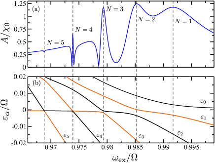
Figure 2: (Color online) (a) Amplitude $A$ of the nonlinear response of the decoupled quantum Duffing detector ($g=0$) as a function of the external driving frequency $\omega_{\rm ex}$. (b) The corresponding quasienergy spectrum $\varepsilon_{\alpha}$. The labels $N$ denote the corresponding $N$-photon (anti-)resonance. The parameters are $\alpha=0.01\Omega$, $f=0.006\Omega$, $T=0.006\Omega$, and $\gamma=1.6\times 10^{-4}\Omega$.

V.1 No coupling between detector and qubit

Before turning to the quantum detection scheme, we discuss the dynamical properties of the isolated detector, which is the quantum Duffing oscillator. A key property is its nonlinearity which generates multiphoton transitions at frequencies $\omega_{\rm ex}$ close to the fundamental frequency $\Omega$. In order to see this, one can consider first the undriven nonlinear oscillator with $f=0$ and identify degenerate states, such as $|n\rangle$ and $|N-n\rangle$ (for $N>n$), when $\delta\Omega=\alpha(N+1)/2$.Dykman05 ; Peano06a ; Peano06b For finite driving $f>0$, the degeneracy is lifted and avoided quasienergy level crossings form, which is a signature of discrete multiphoton transitions in the detector. As a consequence, the amplitude $A$ of the nonlinear response signal exhibits peaks and dips, which depend on whether a large or a small oscillation state is predominantly populated.Peano06a ; Peano06b The formation of peaks and dips goes along with jumps in the phase of the oscillation, leading to oscillations in or out of phase with the driving. A typical example of the nonlinear response of the quantum Duffing oscillator in the deep quantum regime containing few-photon (anti-)resonances is shown in Fig. 2(a) (decoupled from the qubit), together with the corresponding quasienergy spectrum [Fig. 2(b)]. We show the multiphoton resonances up to a photon number $N=5$. The resonances get sharper for increasing photon number, since their widths are determined by the Rabi frequency, which is given by the minimal splitting at the corresponding avoided quasienergy level crossing. Performing a perturbative treatment with respect to the driving strength $f$, one can get the minimal energy splitting at the avoided quasienergy level crossing $(0,N)$ as larsen ; Peano06a

$$\Omega_{N,0}=f\left(\frac{2f}{3\alpha}\right)^{N-1}\frac{\sqrt{(N)!}}{(N-1)!^{2}}.$$ (14)

Because the nonlinearity $\alpha$ is typically fixed by the design of the SQUID, the Rabi frequency can be easily tuned by tuning the driving strength $f$.

V.2 Detector response for weak coupling to the qubit

Next, we consider a finite coupling of the detector to the qubit whose state is to be sensed, i.e., $g\neq 0$. The coupling inevitably induces relaxation and decoherence in the qubit, characterized by the relaxation and dephasing rate, $\Gamma$ and $\Gamma_{d}$, respectively. Typically, the detector couples only weakly to the system, i.e., $g\ll\omega_{\rm qb}$. Then, the associated relaxation and dephasing times ($T_{1}$ and $T_{2}$, respectively) are still much larger than the corresponding relaxation time scale for the detector given by $1/\gamma$. In passing, we note that the corresponding relaxation time around a resonant multiphoton transition (in the underdamped case) has been shown in Refs.  Peano04, ; Peano06b, to be comparable to $\gamma$. Moreover, we bias the qubit with a large asymmetry, $\epsilon\gg\Delta$ in order to “gauge” the detector response.

For a rough evaluation of the order of magnitude of the involved time scales, we may neglect the nonlinearity of the detector ($\alpha=0$) for the moment and estimate the effective relaxation rate for the qubit coupled to an Ohmically damped harmonic oscillator.Thorwart04 This model can be mapped to a qubit coupled to a structured harmonic environment with an effective (dimensionless) coupling constant $\kappa_{\rm eff}=8\gamma g^{2}/\Omega^{2}$. For the realistic parameters used in Fig. 2 and $g=0.0012\Omega$, we find that $\kappa_{\rm eff}\simeq 10^{-10}$, giving rise to an estimated relaxation rateweiss ; Thorwart04 $\Gamma_{\rm harm}\simeq(\pi/2)\sin^{2}(\theta)\,\kappa_{\rm eff}\,\epsilon\simeq 10^{-13}\Omega$ (evaluated at low temperature). Hence, this illustrates that we can easily achieve the situation where $\Gamma_{\rm harm}\ll\gamma$ required for this detection scheme. Then, for a waiting time (after which we start the measurement) much longer than the relaxation time $\gamma^{-1}$ of the nonlinear oscillator, but still smaller than $\Gamma^{-1}$, the oscillator is able to reliably detect the qubit state.

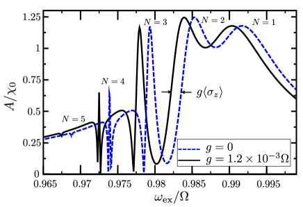
Figure 3: (Color online) Nonlinear response $A$ of the detector as a function of the external driving frequency $\omega_{\rm ex}$ in the presence of a finite coupling $g=0.0012\,\Omega$ to the qubit (black solid line). The blue dashed line indicates the response of the isolated detector. The parameters are the same as in Fig. 2 and $\epsilon=2.2\Omega$ and $\Delta=0.05\Omega$, in correspondence to realistic experimental parameters Lupascu05 .

In fact, under these conditions, the state of the qubit, apart from the inevitable dephasing, remains unaffected in a time window before it reaches its global stationary state and an effective shift of the oscillator’s eigenfrequency arises due to the parametric coupling term $\sim g\cos\theta\,a^{\dagger}a\,\tau_{z}$ in Eq. (6). Treating the qubit-detector interaction term in Eq. (5) perturbatively to lowest order in $g$, the eigenfrequency shift follows straightforwardly as

$$\Omega\rightarrow\Omega+g\,\langle\sigma_{z}\rangle\;.$$

Thus, the nonlinear response is shifted by $-g$ ($+g$) if the qubit is prepared in the state $\sigma_{z}=-1$ ($\sigma_{z}=1$). This is illustrated in Fig. 3, in which we show the nonlinear response of the resonator for the uncoupled (blue dashed line) and the coupled (black solid line) case.

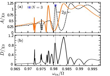
Figure 4: (Color online) (a) Nonlinear response $A$ of the detector coupled to the qubit prepared in its ground state $|\!\!\downarrow\rangle$ (orange solid line) and in its excited state $|\!\!\uparrow\rangle$ (black dashed line) for the same parameters as in Fig. 3. The quadratic qubit-detector coupling induces a global frequency shift of the response by $\delta\omega_{\rm ex}=2g$. (b) Discrimination power $D(\omega_{\rm ex})$ of the detector coupled to the qubit for the same parameters as in a).

For a fixed value of $g$, the shift between the two cases of the opposite qubit states is given by the frequency gap $\delta\omega_{\rm ex}\simeq 2\,g$. Figure 4 (a) shows the nonlinear response of the detector for the two cases when the qubit is prepared in one of its eigenstates: $|\!\!\uparrow\rangle$ (orange solid line) and $|\!\!\downarrow\rangle$ (black dashed line).

An important feature of a detection scheme is that it is efficient in discriminating the states to be detected. This can be quantified by the discrimination power of the detector, which can be defined for our case as

$$D(\omega_{\rm ex})=\left|{A_{|\uparrow\rangle}(\omega_{\rm ex})-A_{|\downarrow\rangle}(\omega_{\rm ex})}\right|\,.$$ (15)

The result for $D(\omega_{\rm ex})$ is shown in Fig. 4 (b). The discrimination power shows a rich structure of local maxima and minima, which indicates that it can be tuned directly by tuning the driving frequency. It is moreover important to realize that the discrimination power can be optimized by tuning $g$. In the optimized case, a local maximum of the multiphoton resonance for one qubit state can be made to coincide with a local minimum of the response for the opposite qubit state yielding to a maximal discrimination power. An example where the discrimination power has been optimized with respect to the three-photon resonance is shown in Fig. 4 (b).

VI Back action in the qubit

Another important prerequisite for a useful detection scheme is that the coupling of the qubit to the detector around a multiphoton resonance does not generate a destructive back action on the qubit dynamics. In this section, we show that the back action in this design is surprisingly small for a realistic choice of parameters.

The back action of the detector on the qubit arises in the form of two contributions from the coupling. First, this coupling has a parametric component ${\cal H}_{1}=g\cos\theta\,n\,\tau_{z}$, which commutes with the Hamiltonian. Thus, in the presence of a coupling of the oscillator to the bath, this term only produces dephasing and no relaxation, as it is, for instance, required for a quantum non-demolition measurement. This part guarantees an efficient detection of the qubit state. The second component ${\cal H}_{2}=g\sin\theta(a^{\dagger\,2}\tau^{-}+a^{2}\tau^{+})/2$ in the coupling term yields transitions in the qubit when two-photon processes are induced in the detector by the external driving and/or by dissipative transition. Since, at low temperature, dissipation is dominated by photon leaking and the driving is very weak, the decay rate of the qubit from its excited state to its ground state accompanied by the emission of two oscillators photons, largely exceeds the excitation rate from the ground state to the excited state accompanied by the absorption of two photons originally coming from the bath or the driving. On the other hand, when the effective oscillator frequency is close to a multiphoton resonance, photon absorption in the coupled system is enhanced and thus the asymptotic qubit population might be reduced.

Thus, for a large asymmetry $|\epsilon|\gg\Delta$, peaks and dips in the qubit population difference $P_{\infty}$ are expected when multiphoton transitions in the detector are induced. This is what is shown in Fig. 5(a), where $P_{\infty}$ is shown for several values of $f$. For an easier orientation, we show in addition the corresponding stationary nonlinear response of the detector in Fig. 5(b). For increasing driving, the deviation from the expected value $P_{\infty}=-1$ becomes more pronounced for larger photon numbers $N$ and larger driving $f$. The reason is that, for increasing driving, a larger Rabi frequency for the corresponding transition results [see Eq. (14)]. From Fig. 5, it follows that when the qubit is prepared in its ground state $|\!\!\uparrow\rangle$ (we consider $\epsilon\gg\Delta$) the back action is very small. The impact is less than $2\%$ for the considered realistic parameters, yielding to a readout contrast of more than $98\%$. This has to be compared with presently achievable readout contrasts of less than $90\%$, Lupascu06 which results from an architecture with a classical Josephson bifurcation amplifier. In passing, we note that the detector response can also be calculated from the stationary solution of the master equation (8), but for the parameters considered here (in particular because of the large qubit bias), this coincides with the shifted one.

Moreover, we note that the components ${\cal H}_{1}$ and ${\cal H}_{2}$ can be tuned by $\epsilon$ and $\Delta$. Therefore, $g\sin\theta$ can in principle be eliminated by setting $\Delta=0$, which would imply that the measurement scheme keeps the state of the qubit without any relaxation but only pure dephasing (ideal quantum nondemolition measurement). However, turning off the splitting implies a major change in the experimental design of the sample, since this parameter is determined by the Josephson energy in the junctions of the superconducting flux qubit and, thus, may not be easy to be realized.

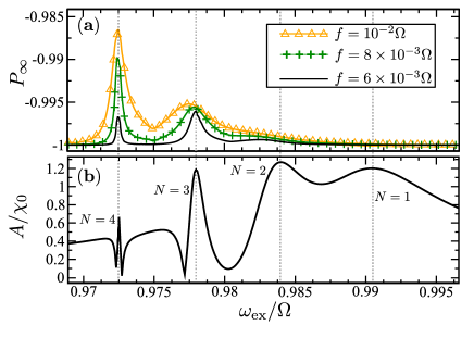
Figure 5: (Color online) (a) Asymptotic population difference $P_{\infty}$ of the qubit states, and (b) the corresponding detector response $A$ as a function of the external frequency $\omega_{\rm ex}$ for the same parameters as in Fig. 3.

The back action of the detector on the qubit should be small not only when the qubit is in its ground state but also when it is in its excited state. We therefore address next the relaxation rate of the qubit. Energy relaxation in the qubit induced by the measurement process will be proportional to the fluctuations of the square of the phase operator $\chi_{+}$ induced by the detector’s environment.Clerk10 ; Lupascu04 This relaxation process is characterized by the transition rate Clerk10 ; Lupascu04

$$\Gamma\simeq\tilde{g}^{2}\,\sin^{2}\theta\,{\cal S}_{\chi_{+}^{2}}[-\omega_{\rm qb}],$$ (16)

which has been computed perturbatively to lowest order in $\tilde{g}$. Here,

$${\cal S}_{\chi_{+}^{2}}[\omega] = \frac{\omega_{\rm ex}}{4\pi}\int_{0}^{2\pi/\omega_{\rm ex}}\!\!\!\!dt\int_{-\infty}^{+\infty}\!\!\!d\tau e^{i\omega\tau}\langle\{\chi^{2}_{+}(\tau+t),\chi^{2}_{+}(t)\}\rangle$$

is the symmetrized power spectrum of $\chi_{+}^{2}$ averaged over the period of the external driving (see Appendix for details), with $\{,\}$ indicating the anticommutator. The fact that information on the qubit state is acquired in the detector via the same channel by which dissipation is introduced is nicely reflected in the expression of the relaxation rate in Eq. (16). In Fig. 6(a), the relaxation rate $\Gamma$ is shown for a large negative asymmetry in the qubit. The relaxation rate is strongly peaked around the multiphoton transitions. There, the noise from the detector absorbs more energy from the qubit around the multiphoton transition $(0,N)$ since the parametric component ${\cal H}_{1}$ of the coupling becomes negligible, leading to a dominant relaxation process induced by ${\cal H}_{2}$.

We emphasize that although the relaxation is maximally enhanced at a multiphoton resonance, the absolute value of $\Gamma$ is still very small in comparison to the damping constant, e.g., $\Gamma/\gamma\sim 10^{-6}$. Thus, we can infer the qubit state with sufficient precision by operating the detector in its steady state regime as it has been assumed in Section V.2.

VII efficiency of the measurement

The measurement of the qubit state requires a coupling to the outer world, which clearly introduces noise to the qubit. In turn, the noisy detector yields measurement results, which are statistically distributed. This implies that several measurements have to be performed to obtain a reliable statistics. Hence, the relaxation time of the qubit state should not only exceed the typical relaxation time of the detector but also the time it takes to acquire sufficient information to infer the qubit state (the measurement time $T_{\rm meas}$). Hence, for a good measurement fidelity, $T_{\rm meas}$ should be smaller than the characteristic time $\Gamma^{-1}$ given by Eq. (16), or, $\Gamma_{\rm meas}/\Gamma\gg 1$.

The measurement time can be formalized Lupascu04 ; Clerk10 ; Makhlin01 as the ratio of the symmetrized power spectrum ${\cal S}_{\chi_{+}}$ of the phase operator $\chi_{+}$ (evaluated at zero frequency) and the square of the difference between the two expectation values of $\chi_{+}$ when the qubit is in the two opposite states, i.e., with Eq. (15),

$$T_{\rm meas}=\frac{{\cal S}_{\chi_{+}}}{[D(\omega_{\rm ex})]^{2}}\,\,.$$ (18)

The result for $T_{\rm meas}$ as a function of $\omega_{\rm ex}$ is shown in Fig. 6 b) for the parameter set used above, for which the discrimination power $D(\omega_{\rm ex})$ around the 3-photon resonance has been maximized. In correspondence with this is the relative minimum of $T_{\rm meas}$ around the 3-photon resonance, see Fig. 6 b). Interestingly enough, the time scale of the measurement time around this resonance is $T_{\rm meas}\approx 10^{-2}\times 2\pi/\Omega$. Considering realistic numbers of a typical experimental set-up Lupascu05 , where $\Omega$ is in the regime of a few GHz, we obtain a time scale of $T_{\rm meas}\approx 100$ ps for the nonlinear quantum detection scheme. This should be contrasted to the measurement time of $T_{\rm meas}\approx 300$ ns obtained in Ref. Lupascu05, . In between the multiphoton resonances, the dependence of $T_{\rm meas}$ on $\omega_{\rm ex}$ shows a rich structure including several singularities, which are simply due to the several crossings of the two nonlinear response curves shown in Fig. 4 a), where $D(\omega_{\rm ex})$ becomes zero, implying insufficient discrimination of the two qubit states.

With this, we can evaluate the measurement efficiency, defined by the ratio $\Gamma_{\rm meas}/\Gamma$, with $\Gamma_{\rm meas}=T_{\rm meas}^{-1}$. This quantity sets the probability to infer the qubit state, based on the nonlinear response of the detector. We show the result for the efficiency of the measurement in Fig.  6(c). Related to the multiphoton resonances in the detector, the efficiency also shows local maxima. For the discrimination power being optimized around the three-photon resonance, the measurement efficiency displays a clear local maximum [see Fig. 6(c)]. Due to the small size of the relaxation rate $\Gamma$ of the detector, the overall measurement efficiency is rather large in comparison to the detection set-up with a linear resonator, Lupascu05 ensuring $\Gamma_{\rm meas}/\Gamma\gg 1$.

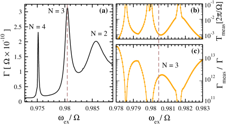
Figure 6: (Color online) (a) Relaxation rate $\Gamma$ of the nonlinear quantum detector, (b) the measurement time $T_{\rm meas}$, and (c) the measurement efficiency $\Gamma_{\rm meas}/\Gamma$ as a function of the external frequency $\omega_{\rm ex}$. The parameters are the same as in Fig. 3.

VIII Conclusions

To conclude, we have introduced a scheme for quantum state detection on the basis of a nonlinear detector which is operated in the regime of resonant few-photon transitions. Discrete multiphoton resonances in the detector can be used to infer the state of the parametrically coupled qubit via a state-dependent frequency shift of the detector’s nonlinear response function. The multiphoton resonances are well separated in the spectrum and sharp enough to allow for a good resolution of the qubit state.

By analyzing key quantities of the detector, we have shown that the nonlinear few-photon detector can be operated efficiently, reliably, and with sufficiently weak back action. In fact, it can be efficiently tuned by tuning the amplitude of the ac bias current of the SQUID. Furthermore, we have shown that the sharpness of the multiphoton resonances can be used to obtain an increased discrimination power as compared to the linear parametric detection scheme. Clearly, the relaxation rate at a multiphoton resonance for the qubit becomes maximal, but in general remains very small. The measurement time around a multiphoton resonance can be tuned such that it becomes minimal. For realistic experimental parameters, we find surprisingly small measurement times, allowing in principle for fast measurements. Moreover, the efficiency of the measurement, which takes the time to acquire enough information to infer the qubit state into account, also assumes large values, thus allowing for a reliable and highly efficient measurement of the qubit state.

We have chosen realistic values for the involved model parameters such that an experimental realization of this quantum measurement scheme should become possible in the near future. The nonlinear detection scheme in the deep few-photon quantum regime offers thus the advantage of an increased discrimination power of more than $98\%$ (for our choice of realistic parameters), as compared to previous classical detection schemes based on the Josephson bifurcation amplifier.

A possible setup in order to realize the nonlinear few-photon detector could be the architecture used in a recent experiment.Murch10 The low-temperature regime, where quantum noise effects are important, has already been reached. In order to operate in the regime of only few photons in the resonator, the sensitivity and stability of the devices might have still to be further increased. However, no principle obstacles are apparent.

*

Appendix A Power spectrum

To calculate the power spectrum of a driven out-off-equilibrium system is a non trivial task, since the time reversal symmetry, which simplifies the calculation in equilibrium systems, is not given anymore. An elegant way to compute this in terms of correlation functions is presented in Ref. Melvin63, . The correlation function between two operators $A$ and $B$ is described as a mean value

$$S_{\rm AB}(t,\tau)={\rm Tr}_{\rm S\oplus B}\{{\cal W}(t+\tau)A(0)\}.$$ (19)

Here, the trace is over the whole system-plus-bath, with the “density” operator ${\cal W}(t+\tau)=U(t+\tau,t)[BW(t)]U^{\dagger}(t+\tau,t)$ and $U(t+\tau,t)=\exp\{-i{\cal T}\int_{t}^{t+\tau}H_{\rm total}(t^{\prime})dt^{\prime}\}$, with $H_{\rm total}$ being the Hamiltonian of the whole system-plus-bath, $W$ the density operator of the total system, and ${\cal T}$ the time ordering operator. Furthermore, $A$ and $B$ are in the Heisenberg representation.

In the regime of weak coupling to the environment, the reduced density operator $\tilde{\varrho}(t+\tau)\equiv{\rm Tr}_{B}\{{\cal W}(t+\tau)\}$ evolves according to the master equation (8).

In the superoperator notation, ${\cal D}_{\alpha\beta,\alpha^{\prime}\beta^{\prime}}=-i(\varepsilon_{\alpha}-\varepsilon_{\beta})\delta_{\alpha\alpha^{\prime}}\delta_{\beta\beta^{\prime}}+{\cal L}_{\alpha\beta,\alpha^{\prime}\beta^{\prime}}$ (Liouville superoperator) is represented by a ${\cal N}^{2}\times{\cal N}^{2}$ supermatrix ${\bf\cal D}$, where ${\cal N}$ is the number of effective states in the system. In the same way, the density operator $\varrho_{\alpha\beta}$ formally is a ${\cal N}^{2}$ dimensional column vector $\varrho(t)$. The solution of the master equation is reduced to an eigenvalue problem of the matrix ${\bf\cal D}$, as

$${\bf\cal D}\cdot{\bf v}^{m}=\Gamma_{m}{\bf v}^{m},\quad{\bf v}^{\dagger}_{m}\cdot{\bf\cal D}=\Gamma_{m}{\bf v}^{\dagger}_{m},$$ (20)

where ${\bf v}^{m}$ and ${\bf v}_{m}$ are the left and right eigenvectors, respectively, with eigenvalue $\Gamma_{m}$.

In the superoperator notation, the master equation (8) is expressed as $\dot{\varrho}(t)={\bf\cal D}\cdot{\varrho}(t)$, and its solution is given by

$$\varrho(t)=\exp\{{\bf\cal D}\,t\}\cdot\varrho(t=t_{0}).$$ (21)

In the regime of the RWA, and at low temperature the master equation (8) conserves the trace and the positivity of the density operator, i.e., it assumes Lindblad form. Therefore, we can expand the solution of the master equation in terms of the right-eigenvector ${\bf v}^{m}$

$$\varrho(t)=\sum_{m}{\bf v}^{m}\,c_{m}\exp\{{\Gamma_{m}\,t}\},$$ (22)

with $c_{m}={\bf v}^{\dagger}_{m}\cdot\varrho(t_{0})$. Here, we have used the orthogonality property ${\bf v}_{m}^{\dagger}\cdot{\bf v}^{m^{\prime}}=\delta_{mm^{\prime}}$. The corresponding expression follows for the operator $\tilde{\varrho}(t+\tau)$, but with a different initial condition. It is easily understandable in the operator notation

$$\tilde{\varrho}_{\alpha\beta}(t+\tau)=\sum_{m,\alpha^{\prime}\beta^{\prime}\xi^{\prime}}v^{m}_{\alpha\beta}\;v^{\dagger}_{m,\beta^{\prime}\alpha^{\prime}}\;B_{\alpha^{\prime}\xi^{\prime}}(t)\;\varrho_{\xi^{\prime}\beta^{\prime}}(t)\;e^{\Gamma_{m}\tau}$$ (23)

where $B_{\alpha\beta}(t)=\langle\phi_{\alpha}(t)|B|\phi_{\beta}(t)\rangle$, and $v^{m}_{\alpha\beta}$ ($v_{m,\alpha\beta}$) is the operator representation of ${\bf v}^{m}$ (${\bf v}_{m}$) in the quasienergy states. Considering an initial time in the stationary regime, i.e., $\varrho_{\alpha\beta}(t)\rightarrow\varrho^{\infty}_{\alpha\beta}$, and after averaging the initial time $t$ over the period $2\pi/\omega_{\rm ex}$, the correlation function reads

$$S_{\rm AB}(t)=\sum_{m,n}\;S_{nm}\;e^{\Gamma_{m}t-in\omega_{\rm ex}t},$$ (24)

with

$$S_{nm}=\sum_{\alpha\beta}\sum_{\alpha^{\prime}\beta^{\prime}\xi^{\prime}}\;v^{m}_{\alpha\beta}\;A_{\beta\alpha,n}\;v^{\dagger}_{m,\beta^{\prime}\alpha^{\prime}}\;B_{\alpha^{\prime}\xi^{\prime},-n}\;\rho^{\infty}_{\xi^{\prime}\beta^{\prime}},$$ (25)

where $A_{\alpha\beta,n}$ and $B_{\alpha\beta,n}$ are the coefficients of the Fourier expansion of $A_{\alpha\beta}(t)$ and $B_{\alpha\beta}(t)$, respectively. The power spectrum is obtained directly from the Fourier transform of Eq. (24).

References

- (1) A. A. Clerk, M.H. Devoret, S.M. Girvin, F. Marquardt, and R.J. Schoelkopf, Rev. Mod. Phys. 82, 1155 (2010).
- (2) A. Lupaşcu, C.J.M. Verwijs, R.N. Schouten, C.J.P.M. Harmans, and J.E. Mooij, Phys. Rev. Lett. 93, 177006 (2004).
- (3) A. Lupaşcu, C. J. P. M. Harmans, and J. E. Mooij, Phys. Rev. B 71, 184506 (2005).
- (4) I. Siddiqi, R. Vijay, F. Pierre, C. M. Wilson, M. Metcalfe, C. Rigetti, L. Frunzio, and M. H. Devoret , Phys. Rev. Lett. 93, 207002 (2004).
- (5) R. Vijay, M.H. Devoret, and I. Siddiqi, Rev. Sci. Instrum. 80, 111101 (2009).
- (6) A. H. Nayfeh and D. T. Mook, Nonlinear Oscillations (Wiley, New York, 1979).
- (7) A. Lupaşcu, E.F.C. Driessen, L. Roschier, C.J.P.M. Harmans, and J. E. Mooij, Phys. Rev. Lett. 96, 127003 (2006).
- (8) M. I. Dykman and M. A. Krivoglaz, Zh. Eksp. Teor. Fiz. 77, 60 (1979) [Sov. Phys. JETP 50, 30 (1979)].
- (9) M. I. Dykman and V. N. Smelyanski, Phys. Rev. A 41, 3090 (1990).
- (10) A. P. Dmitriev and M. I. D’yakonov, Zh. Eksp. Teor. Fiz. 90, 1430 (1986) [Sov. Phys. JETP 63, 838 (1986)].
- (11) M. I. Dykman and V.N. Smelyanskii, Zh. Eksp. Teor. Fiz. 94, 61 (1988) [Sov. Phys. JETP 67, 1769 (1988)].
- (12) V. Peano and M. Thorwart, Phys. Rev. B 70, 235401 (2004).
- (13) V. Peano and M. Thorwart, New J. Phys. 8, 21 (2006).
- (14) V. Peano and M. Thorwart, Chem. Phys. 322, 135 (2006).
- (15) K. W. Murch, R. Vijay, I. Barth, O. Naaman, J. Aumentado, L. Friedland, and I. Siddiqi, Nature Phys. 7, 105 (2010).
- (16) O. Naaman, J. Aumentado, L. Friedland, J. S. Wurtele, and I. Siddiqi, Phys. Rev. Lett. 101, 117005 (2008).
- (17) J. E. Mooij, T.P. Orlando, L. Levitov, L. Tian, and C. H. van der Wal, Science 285, 1036 (1999).
- (18) O.H. Soerensen, J. Appl. Phys. 47, 5030 (1976).
- (19) C. D. Tesche and J. Clarke, Low Temp. Phys. 29, 301 (1977).
- (20) Y. Makhlin, G. Schön, and A. Shnirman, Rev. Mod. Phys. 73, 357 (2001).
- (21) P. Bertet, I. Chiorescu, G. Burkard, K. Semba, C. J. P. M. Harmans, D. P. DiVincenzo, and J. E. Mooij, Phys. Rev. Lett. 95, 257002 (2005).
- (22) U. Weiss, Quantum Dissipative Systems, 3rd ed. (World Scientific, Singapore, 2007).
- (23) V. Peano and M. Thorwart, Europhys. Lett. 89, 17008 (2010).
- (24) L. S. Bishop, J. M. Chow, J. Koch, A. A. Houck, M. H. Devoret, E. Thuneberg, S. M. Girvin, and R. J. Schoelkopf, Nature Phys. 5, 105 (2009).
- (25) D. M. Larsen and N. Bloembergen, Opt. Comm. 17, 254 (1976)
- (26) M. I. Dykman and M. V. Fistul, Phys. Rev. B 71, 140508 (2005).
- (27) M. Thorwart, E. Paladino, and M. Grifoni, Chem. Phys. 296, 333 (2004).
- (28) M. Lax, Rev. Phys. 129, 2342 (1963).