Temporal effects in the growth of networks

Abstract

We show that to explain the growth of the citation network by preferential attachment (PA), one has to accept that individual nodes exhibit heterogeneous fitness values that decay with time. While previous PA-based models assumed either heterogeneity or decay in isolation, we propose a simple analytically treatable model that combines these two factors. Depending on the input assumptions, the resulting degree distribution shows an exponential, log-normal or power-law decay, which makes the model an apt candidate for modeling a wide range of real systems.

Over the years, models with preferential attachment (PA) were independently proposed to explain the distribution of the number of species in a genus Yule25 , the power-law distribution of the number of citations received by scientific papers Price76 and the number of links pointing to WWW pages BarAlb99 . A theoretical description of this class of processes and the observation that they generally lead to power-law distributions are due to Simon Simon55 . Notably, the application of PA to WWW data by Barabási and Albert helped to initiate the lively field of complex networks Newman03 . Their network model, which stands at the center of attention of this work, was much studied and generalized to include effects such as presence of purely random connections Liu02 , non-linear dependence on the degree KrReLe00 , node fitness BiaBar01 and others (AlbBar02, , Ch. 8).

Despite its success in providing a common roof for many theoretical models and empirical data sets, preferential attachment is still little developed to take into account the temporal effects of network growth. For example, it predicts a strong relation between a node’s age and its degree. While such first-mover advantage Newman09 plays a fundamental role for the emergence of scale free topologies in the model, it is a rather unrealistic feature for several real systems (e.g., it is entirely absent in the WWW AdaHub00 and significant deviations are found in citation data Newman09 ; Redner05 ). This motivates us to study a model of a growing network where a broad degree distribution does not result from strong time bias in the system. To this end we assign fitness to each node and assume that this fitness decays with time—we refer it as relevance henceforth. Instead of simply classifying the vertices as active or inactive, as done in AmScBaSt00 ; LeJaLa05 , we use real data to investigate the relevance distribution and decay therein and build a model where decaying and heterogeneous relevance are combined.

Models with decaying fitness values (“aging”) were shown to produce narrow degree distributions (except for very slow decay) DoMe00 and widely distributed fitness values were shown to produce extremely broad distributions or even a condensation phenomenon where a single node attracts a macroscopic fraction of all links BiaBar01b . We show that when these two effects act together, they produce various classes of behavior, many of which are compatible with structures observed in real data sets.

Before specifying a model and attempting to solve it, we turn to data to provide support for our hypothesis of decaying relevance. We use here the citation data provided by the American Physical Society (APS) which contains all 450 084 papers published by the APS from 1893 to 2009 together with their 4 691 938 citations of other papers from APS journals. It is particularly fitting to use citation data for our work because ordinary PA with direct proportionality to the node degree was detected in this case by previous works Newman09 ; JeNeBa03 . Data analysis according to CSN09 reveals that the best power-law fit to the in-degree data has lower bound $k_{\mathrm{min}}=50$ and exponent $2.79\pm 0.01$. Though $p$-values greater than $0.10$ are only achieved for $k_{\mathrm{min}}\gtrsim 150$, log-normal distribution does not appear to fit the data particularly better. Since PA can be best imagined to model citations within one field of research, we consider in our analysis also a subset of papers about the theory of networks. We identify them using the PACS number 89.75.Hc (“Networks and genealogical trees”)—in this way we obtain a small data set with 985 papers and 4 395 citations among them.

Denoting the in-degree of paper $i$ at time $t$ as $k_{i}(t)$ and assuming that during next $\Delta t$ days, $C(t,\Delta t)$ new citations are added to papers in the network, preferential attachment predicts that the number of citations received by paper $i$ is $\Delta k_{i}(t,\Delta t)_{PA}=C(t,\Delta t)k_{i}(t)/\sum_{j}k_{j}(t)$. If in reality, $\Delta k_{i}(t,\Delta t)$ citations are received, the ratio between this number and the expected number of received citations defines the paper’s relevance

$$X_{i}(t,\Delta t):=\frac{\Delta k_{i}(t,\Delta t)\sum_{j}k_{j}(t)}{C(t,\Delta t)k_{i}(t)}.$$ (1)

This expression is obviously undefined for $k_{i}(t)=0$ which stems from the known limitation of the PA in requiring an additional attractiveness factor to allow new papers to gain their first citation. Although one could try to include this effect in our analysis, we simply compute $X_{i}(t,\Delta t)$ only when $k_{i}(t)\geq 1$. Similarly we exclude time periods when no citations are given and $C(t,\Delta t)=0$.

Figure 1 shows how the average relevance of papers with different final in-degree values decays with time after their publication. We see that the relevance values indeed decay and this decay is initially very fast (for papers with the highest final in-degree, it is by a factor of 100 in less than three years). However, the exponential decay reported in Zhu03 appears to have only very limited validity (up to five years after the publication date). After 10 or more years, the decay becomes very slow or even vanishes, producing a stationary relevance value $r_{0}$. Figure 2 depicts the distribution of the total relevance $X_{T}(i)=\sum_{t}X_{i}(t)$ and shows that, perhaps contrary to one’s expectations, this distribution is rather narrow with an exponential decay for $X_{T}\gtrsim 25\cdot 10^{3}$. An exponential-like tail appears also when the analysis is restricted to papers of a similar age which means that it is not only an artifact of the papers’ age distribution. One could attempt to fit this data with, for example, a Weibull distribution as in BoMaGo04 . We shall see later that it is the tail behavior of $X_{T}$ what determines the tail behavior of the degree distribution, hence the current level of detail suffices our purpose. We can conclude that in the studied citation data, relevance values exhibit time decay and papers’ total relevances are rather homogeneously distributed, showing an exponential decay in the tail.

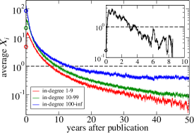
Figure 1: Time decay of the average relevance values (based on $\Delta t=91\,\mathrm{days}$) for papers divided into groups according to their final in-degree (color online). The dashed line shows $X=1$ indicating exact preferential attachment and open circles show the initial relevance values. The inset shows results for papers about the theory of networks.

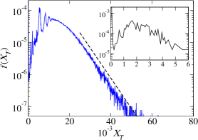
Figure 2: The distribution of the total relevance $X_{T}$ in the studied data (color online). For $X_{T}\gtrsim 25\cdot 10^{3}$, $f(X_{T})$ decays as $\exp[-\alpha X_{T}]$ with $\alpha=(21.7\pm 0.2)\cdot 10^{-3}$ (denoted with the indicative dashed line). The peak at $X_{T}=0$ is due to approximately $60\,000$ papers without citations. The inset shows results for papers about the theory of networks.

Now we proceed to a model based on the above-reported empirical observations. We consider a uniformly growing undirected network which initially consists of two connected nodes. At time $t$, a new node is introduced and linked to an existing node $i$ where the probability of choosing node $i$ is

$$P(i,t)=\frac{k_{i}(t)R_{i}(t)}{\sum_{j=1}^{t}k_{j}(t)R_{j}(t)}$$ (2)

which has the same structure as assumed before in DoMe00 ; Zhu03 . Here $k_{j}(t)$ and $R_{j}(t)$ is degree and relevance of node $j$ at time $t$, respectively footnote1 . Our goal is to determine whether a stationary degree distribution exists and find its functional form.

Eq. (2) represents a complicated system where evolution of each node’s degree depends not only on the node itself but also on the current degrees and relevances of all other nodes. The key simplification is based on the assumption that at any time moment (except for a short initial period), there are many nodes with non-negligible values of $k_{i}(t)R_{i}(t)$. The denominator of Eq. (2) is then a sum over many contributing terms and therefore it fluctuates little with time. This allows us to approximate the exact selection probability $P(i,t)$ with

$$P(i,t)=\frac{k_{i}(t)R_{i}(t)}{\Omega(t)}$$ (3)

where $\Omega(t)$ is now just a normalization factor.

If $R_{i}(t)$ decays sufficiently fast (faster than $1/t$) and $\lim_{t\to\infty}R_{i}(t)=0$, the initial growth of $\Omega(t)$ stabilizes at a certain value $\Omega^{*}$ which shall be determined later by the requirement of self-consistency. The master equation for the degree distribution $p(k_{i},t)$ now has the form $p(k_{i},t+1)=(1-k_{i}R_{i}(t)/\Omega^{*})p(k_{i},t)+(k_{i}-1)R_{i}(t)p(k_{i}-1,t)/\Omega^{*}$. Note that the stationarity of $p(k_{i},t)$ in our case is due to transition probabilities that vanish because $\lim_{t\to\infty}R_{i}(t)=0$. Before tackling the degree distribution itself, we examine the expected final degree of node $i$, $\langle k_{i}^{F}\rangle$. By multiplying the master equation with $k_{i}$ and summing it over all $k_{i}$, we obtain a difference equation $\langle k_{i}(t+1)\rangle=\langle k_{i}(t)\rangle\big{(}1+R_{i}(t)/\Omega^{*}\big{)}$. If $R_{i}(t)$ decays sufficiently slowly, we can switch to continuous time to obtain $\mathrm{d}\langle k_{i}(t)\rangle/\mathrm{d}t=k_{i}(t)R_{i}(t)/\Omega^{*}$ which together with $\langle k_{i}(t_{i})\rangle=1$ yields

$$\langle k_{i}^{F}\rangle=\exp\Big{(}\frac{1}{\Omega^{*}}\int_{t_{i}}^{\infty}\!R_{i}(t)\,\mathrm{d}t\Big{)}.$$ (4)

Here $t_{i}$ is the time when node $i$ is introduced to the system (in our case, $t_{i}=i$). When the continuum approximation is valid, this result is well confirmed by numerical simulations (see the inset in Fig. 3). To observe saturation of the degree growth for an infinitely growing network, the total relevance $T_{i}:=\int_{t_{i}}^{\infty}R_{i}(t)\,\mathrm{d}t$ must be finite and hence $R_{i}(t)$ must decay faster than $1/t$ for all nodes. To assess the error of the continuum approximation, one can use the Taylor expansion to write $\langle k_{i}(t+1)\rangle-\langle k_{i}(t)\rangle\approx\mathrm{d}\langle k_{i}(t)\rangle/\mathrm{d}t+\tfrac{1}{2}\mathrm{d}^{2}\langle k_{i}(t)\rangle/\mathrm{d}t^{2}$. The second derivative term can be approximately evaluated using Eq. (4) and it can be shown that it’s negligible when $\lvert\dot{R}_{i}(t)\rvert\ll R_{i}(t)$, which is consistent with our initial assumption that $R_{i}(t)$ decays sufficiently slowly for all $i$.

Since $\Omega^{*}$ is the same for all nodes, Eq. (4) demonstrates that a node’s expected final degree depends only on its total relevance $T_{i}$. Therefore we can use the continuum approach to compute $\Omega^{*}$ directly from its definition as $\Omega^{*}=\int\varrho(T)\langle\Omega(T)\rangle\,\mathrm{d}T$ where $\langle\Omega(T)\rangle\approx\lim_{t\rightarrow\infty}\int_{0}^{t}R(t-t_{0})\langle k(t-t_{0})\rangle\,\mathrm{d}t_{0}=\int_{0}^{\infty}R(t)\langle k(t)\rangle\,\mathrm{d}t=\Omega^{*}\big{(}\mathrm{e}^{T/\Omega^{*}}-1\big{)}$, as there is only one node with total relevance $T$ which contributes to $\langle\Omega(T)\rangle$ with $R(t)\langle k(t)\rangle$ for each $t$. When $\varrho(T)$ is given, the resulting equation

$$\int\varrho(T)\,\mathrm{e}^{T/\Omega^{*}}\mathrm{d}T=2$$ (5)

can be used to find $\Omega^{*}$. Alternatively, the construction constraint of the average network’s degree in the large time limit, $\langle k\rangle=2$, implies $\int_{0}^{\infty}\varrho(T)\langle k^{F}(T)\rangle\,\mathrm{d}T=2$ which gives the same equation for $\Omega^{*}$. Note that when $\varrho(T)$ decays slower than exponentially, the integral in Eq. (5) diverges and no $\Omega^{*}$ can satisfy the system’s requirements, implying that in this case no stationary value of $\Omega^{*}$ is established.

Similarly to $\langle k_{i}(t)\rangle$, degree fluctuations for nodes of a given total relevance can be derived from the master equation. When $\lvert\dot{R}_{i}(t)\rvert\ll R_{i}(t)$, the continuum approximation can be again shown to be valid and yields

$$\mathrm{d}\langle k_{i}^{2}\rangle/\mathrm{d}t=R_{i}(t)\big{(}\langle k_{i}(t)\rangle+2\langle k_{i}^{2}(t)\rangle\big{)}/\Omega^{*}$$ (6)

where $\langle k_{i}^{2}(0)\rangle=1$ and which can be solved for general $R_{i}(t)$ to obtain the stationary standard deviation of the node’s degree

$$\sigma_{k}(T_{i})=\big{(}\mathrm{e}^{2T_{i}/\Omega^{*}}-\mathrm{e}^{T_{i}/\Omega^{*}}\big{)}^{1/2}.$$ (7)

When $T_{i}=T$ for all nodes, Eq. (5) implies $\mathrm{e}^{T/\Omega^{*}}=2$ and therefore $\sigma_{k}=\sqrt{2}$. We see that the resulting degree distribution $f(k)$ is very narrow which is not the case in most real complex networks. One has to proceed to heterogeneous $T_{i}$ values.

Since the distribution $f(k_{i}|T_{i})$ is very narrow, one can use the distribution $\varrho(T)$ together with Eq. (4) and $f(k)\,\mathrm{d}k=\varrho(T)\,\mathrm{d}T$ to obtain the degree distribution $f(k)$. If $T_{i}$ are drawn from a distribution with finite support, the support of $f(k)$ is also finite which is not of interest for us (though it may be appropriate to model some systems). If $T_{i}$ follow a truncated normal distribution (the truncation is needed to ensure $T_{i}\geq 0$ and $\langle k_{i}\rangle\geq 1$), it follows immediately that $f(k)$ is log-normally distributed which may be of great relevance in many cases CSN09 ; Mitz04 . We finally consider $T_{i}$ values that follow a fast-decaying exponential distribution $\varrho(T)=\alpha\exp[-\alpha T]$ which is supported by the analysis of citation data presented in Figure 2. By transforming from $\varrho(T)$ to $f(k)$, we then obtain $f(k)\sim k^{-1-\alpha\Omega^{*}}$. From Eq. (5) it follows that in this case is $\Omega^{*}=2/\alpha$, hence the power-law exponent is $\gamma=3$. We see that even a very constrained exponential distribution of $T$ leads to a scale-free distribution of node degree—the exponent of this distribution is in fact the same as in the original PA model. As shown in Fig. 3, numerical simulations confirm that this result truly realizes in a wide range of parameters.

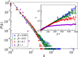
Figure 3: Simulation results for the studied model where $R_{i}(t)=R_{i}(0)\,\mathrm{e}^{-\beta(t-t_{i})}$ ($t_{i}$ is the time when node $i$ entered the network), $R_{i}(0)$ values are drawn from an exponential distribution and the final number of nodes is $10^{5}$ (color online). Since the decay is the same for all nodes, distributions of $R_{i}(0)$ and $T_{i}$ have the same functional form. The indicative dashed line has the slope of $-3$. The inset shows the dependency between $\beta T$ and the average node degree; the dashed line follows from Eq. (4).

Motivated by Fig. 2, one may ask what happens when $T$ is exponentially distributed only in its tail. We take a simple combination where $1-q$ of all nodes have $T=1$ and the remaining nodes follow the exponential distribution $\varrho(T)=\mathrm{e}^{-(T-1)}$ for $T\in[1;\infty)$. By the same approach as before, we obtain the equation for $\Omega^{*}$ in the form $\mathrm{e}^{1/\Omega^{*}}[1-q+q/(1-1/\Omega^{*})]=2$ which yields power-law exponents monotonically increasing from $2.44$ (for $q=0$) to $4.18$ (for $q=1$). The reason for the exponent decreasing as $q$ shrinks is that when $q$ is small, every node with a potentially high exponentially-distributed $T$ value has few able competitors during its life span and therefore it is likely to acquire many links (more than for $q=1$). At the same time, as $q$ decreases, the power-law tail contains smaller and smaller fraction of all nodes and becomes less visible. This example further demonstrates flexibility of the studied model which is able to produce different kinds of behavior depending on the input parameters.

It is easy to show that as long as $R_{i}(t)$ values decay faster than $1/t$, the growth of $k_{i}(t)$ is sublinear and the condensation phase observed in BiaBar01b is not possible despite $T$ having an unlimited support. However, in the system numerically studied in Fig. 3, deviations from the scale free distribution of node degree appear when $\beta$ is small. This happens when the characteristic lifetime of a node, $1/\beta$, is so long that the decay cannot compensate for the unlimited support of $\varrho(T)$. To get a qualitative estimate for the value of $\beta$ when these deviations appear, we use the following argument. If the final degree distribution is a power law with exponent $\gamma$, we expect $\langle k_{\mathrm{max}}\rangle$ to grow as $t^{1/(\gamma-1)}=\sqrt{t}$ (here we use that the number of nodes equals $t$). When a node with a sufficiently high relevance appears, the system can undergo a temporary condensation phase where this node acquires a finite fraction of links during its lifetime. To avoid a deviation from the power law behavior, this lifetime must not be longer than $\langle k_{\mathrm{max}}\rangle$, hence $\beta\lesssim 1/\sqrt{t}$. As $t$ goes to $\infty$, $\beta$ can be arbitrarily small and yet no deviations appear. This confirms that in the thermodynamic limit, the condensation phase does not realize in our model.

The key formula (4) builds on the assumption that fluctuations of $\Omega(t)$ are small enough, and the degree distribution results hold if the effective lifetime of nodes is long enough (a short-living node cannot acquire many links regardless of its total relevance). These two assumptions are in fact closely related: when the effective lifetime of nodes is long, then at any time step there are many nodes competing for the incoming link and the time fluctuations of $\Omega(t)$ are hence small. To evaluate the effective life time of node $i$, $\tau_{i}$, we use the participation number

$$\tau_{i}:=\frac{\big{(}\sum_{t=1}^{\infty}R_{i}(t)\big{)}^{2}}{\sum_{t=1}^{\infty}R_{i}(t)^{2}}\approx T_{i}^{2}/\int_{0}^{\infty}R_{i}(t)^{2}\,\mathrm{d}t.$$ (8)

When $\tau_{i}\gg 1$ for all nodes, $\Omega(t)$ fluctuates little. Numerical simulations show that $\mathrm{var}(\Omega)$ is indeed proportional to the effective life time for a wide range of decay functions $R(t)$, confirming its relevance in the present context. In conclusion, our analytical results are valid when all the obtained conditions ($R_{i}(t)$ decreasing faster than $1/t$, $\lvert\dot{R}_{i}(t)\rvert\ll R_{i}(t)$, and $\tau_{i}\gg 1$), are fulfilled.

To summarize, we studied a model of a growing network where heterogeneous fitness (relevance) values and aging of nodes (time decay) are combined. We showed that in contrast to models where these two effects are considered in isolation, here we obtain various realistic degree distributions for a wide range of input parameters. We analyzed real citation data and showed that they indeed support the hypothesis of coexisting node heterogeneity and time decay. Even when our model is more realistic than the preferential attachment alone, it neglects several effects which might be of importance in various systems: directed nature of the network, accelerating growth of the network, gradual fragmentation of the network into related yet independent fields, and others. Note that the very reason for the exponential tail of the total fitness value $T$, though it is crucial for the resulting degree distribution, is not discussed here at all—yet we have empirical support for it in our data. Also the case when the normalization $\Omega(t)$ in Eq. (2) does not have a stationary value (because $\lim_{t\to\infty}R_{i}(t)>0$ or $\varrho(T)$ decays slower than exponentially) is open. Finally, note that while we focused on the degree distribution here, there are other network characteristics—such as clustering coefficient and degree correlations—that deserve further attention.

This work was supported by the EU FET-Open Grant 231200 (project QLectives) and by the Swiss National Science Foundation Grant 200020-132253. We are grateful to the APS for providing us the data set. We acknowledge helpful discussions with Yi-Cheng Zhang, An Zeng, Juraj Földes, Matouš Ringel and Yves Berset.

References

- (1) G. U. Yule, Phil. Trans. R. Soc. B 213, 21 (1925).
- (2) D. J. de S. Price, J. of the Am. Soc. for Inf. Science 27, 292 (1976).
- (3) H. A. Simon, Biometrika 42, 425 (1955).
- (4) A. L. Barabási, R. Albert, Science 286, 509 (1999).
- (5) M. E. J. Newman, SIAM Review 45, 167 (2003).
- (6) Z. Liu, Y.-C. Lai, N. Ye, P. Dasgupta, Phys. Lett. A 303, 337 (2002).
- (7) P. L. Krapivsky, S. Redner, F. Leyvraz, Phys. Rev. Lett. 85, 4629 (2000).
- (8) G. Bianconi, A.-L. Barabási, EPL 54, 436 (2001).
- (9) R. Albert, A.-L. Barabási, Revs. of Mod. Phys. 74, 47 (2002).
- (10) M. E. J. Newman, EPL 86, 68001 (2009).
- (11) L. A. Adamic, B. A. Huberman, Science 287, 2115 (2000).
- (12) S. Redner, Phys. Today 58, No. 6, 49 (2005).
- (13) L. A. N. Amaral, A. Scala, M. Barthélémy, H. E. Stanley, Proc. Natl. Acad. Sci. U. S. A. 97, 11149 (2000).
- (14) S. Lehmann, A. D. Jackson, B. Lautrup, EPL 69, 298 (2005).
- (15) S. N. Dorogovtsev, J. F. F. Mendes, Phys. Rev. E 62, 1842 (2000).
- (16) G. Bianconi, A.-L. Barabási, Phys. Rev. Lett. 86, 5632 (2001).
- (17) H. Jeong, Z. Néda, A. L. Barabási, EPL 61, 567 (2003).
- (18) A. Clauset, C. R. Shalizi, M. E. J. Newman, SIAM Review 51, 661 (2009).
- (19) H. Zhu, X. Wang, J.-Y. Zhu, Phys. Rev. E 68, 056121 (2003).
- (20) Note that our definition of is consistent in the sense that when these values are used in Eq. (2), the expected degree increments equal the observed ones.
- (21) Katy Börner, J. T. Maru, R. L. Goldstone, Proc. Natl. Acad. Sci. U. S. A. 101, 5266 (2004).
- (22) M. Mitzenmacher, Internet Mathematics 1, 226 (2008).