Radiative decays () in little Higgs models
Abstract
The study of the phenomenology of an extra neutral gauge boson, , can help us to unravel the underlying theory. We study the decay of such a particle into two neutral gauge bosons, (), in two popular versions of the little Higgs model: the littlest Higgs model (LHM) and the simplest little Higgs model (SLHM). These decays are induced at the one-loop level by a fermion triangle and are interesting as they are strongly dependent on the mechanism of anomaly cancellation. All the relevant tree-level two- and three-body decays of the gauge boson are also calculated. It is found that the branching ratios for the decays can be as large as that of a tree-level three-body decay but the decay is very suppressed. We also discuss the experimental prospects for detecting these decays at the LHC and a future linear collider. We conclude that the latter would offer more chances for the detection of such rare decays.
pacs:
14.70.Pw,13.38.DgI Introduction
The standard model (SM) of electroweak interactions has proven highly successful as its predictions have been confirmed with a high precision at particle colliders. The only missing ingredient of this theory is the Higgs boson, which plays an essential role in the mechanism of electroweak symmetry breaking (EWSB). A global fit to electroweak precision data collected at LEP and Tevatron :2005dia suggests that the Higgs boson mass, , is below 209 GeV. Since receives quadratically divergent contributions at the one-loop level from the top quark, the gauge bosons, and the Higgs boson itself, fine-tuning would be required to get a relatively light . The problem would worsen if the new physics scale was of the order of the Planck scale. This is known as the little hierarchy problem, which remains among the unanswered puzzles of the SM. Although supersymmetry has long been known as a promising prospect to solve the hierarchy problem, very recently little Higgs models ArkaniHamed:2001nc ; ArkaniHamed:2002qy ; ArkaniHamed:2002pa ; ArkaniHamed:2002qx ; Low:2004xc ; Kaplan:2003uc ; Schmaltz:2004de have emerged as an interesting alternative to stabilize the Higgs boson mass without fine-tuning. This class of theories are based on the old hypothesis that the Higgs boson is a pseudo-Goldstone boson arising from a spontaneously broken approximate global symmetry at a scale of the order of a few TeVs. After a collective symmetry breaking mechanism is introduced, there is a set of new particles that play the role of partners of the SM gauge bosons and the top quark. The couplings of these new particles are such that the quadratic divergences to arising at one-loop from the SM particles are exactly canceled by the contribution of their respective partners, thereby yielding a naturally light Higgs boson. Several realizations of this idea have been proposed in the literature, such as the littlest Higgs model (LHM) ArkaniHamed:2002qy , the littlest Higgs model with T-parity (LHTM) Low:2004xc , which is actually an extension of the latter, and the simplest little Higgs model (SLHM) Kaplan:2003uc ; Schmaltz:2004de .
Little Higgs models predict effects that may show up at the 1 TeV level, so the study of their phenomenology could be at the reach of the large hadron collider (LHC) or a future linear collider. The scale of the global symmetry breaking as well as other parameters of little Higgs models have been constrained from low energy electroweak measurements Csaki:2002qg ; Hewett:2002px ; Csaki:2003si ; Gregoire:2003kr ; Chen:2003fm ; Casalbuoni:2003ft ; Marandella:2005wd ; Han:2005dz ; Kilian:2003xt ; Hubisz:2005tx and the respective phenomenology has been widely studied throughout the last years Burdman:2002ns ; Han:2003wu ; Han:2005ru ; Hubisz:2004ft ; Belyaev:2006jh ; Freitas:2006vy . Even if the new particles predicted by little Higgs models were too heavy to be directly produced at particle colliders, they could show-up via loop effects in particle observables. Apart from reproducing the SM at the electroweak scale, little Higgs models predict heavy partners for the top quark and the weak gauge bosons, which are necessary to cancel the quadratic divergences of the Higgs boson mass at the one-loop level. There can also be a massive partner for the photon, as well as new scalar particles and additional fermions, but their presence is more dependent on the particular implementation of the model. In this work we will concentrate our attention on the extra neutral gauge boson that is the partner of the SM weak gauge boson. As explained below, it can give a more robust signal of the model at particle colliders than a heavy photon.
An extra neutral gauge boson arises in models in which the SM group is extended with an extra gauge group or if it is embedded into a larger gauge group, such as occurs in the left-right symmetric model, grand unified theories, 331 models, extra dimension theories, technicolor models, the twin-left right symmetric model, etc. It is worth mentioning that the literature has been mainly devoted to the study of the extra neutral gauge boson associated with an extra gauge group Langacker:2008yv , which is customarily denoted by . In the LHM and its T-parity extension, the gauge boson partner, denoted by , is associated with the additional gauge group. In these models there is also a heavy photon partner, , which is the lightest new particle and is the analogue of the gauge boson. Although this gauge boson has a great potential to hint the first LHM evidences at a particle collider, it has been argued that it would not offer a robust signal of the model due to the arbitrariness of the charge assignments of the SM fermions under the gauge group. As far as the SLHM is concerned, the role of the partner, which is denoted by , is played by a linear combination of and gauge fields. This model also predicts a new no self conjugate extra neutral gauge boson, . From now on, the letter will denote the extra neutral gauge boson that plays the role of the partner of the gauge boson in little Higgs models. When we refer to a particular model version, we will use the customary notation to refer to this extra neutral gauge boson.
It is not possible to obtain a model-independent bound on the mass of an extra neutral gauge boson from experimental measurements, but electroweak precision data Erler:1999nx along with Tevatron :2007sb and LEP2 Alcaraz:2006mx searches, allow one to obtain limits on from about GeV to GeV in models with universal flavor gauge couplings. Since the mass of the new heavy gauge bosons predicted by little Higgs models are of the the order of , a bound on translates into an indirect bound on . While an extra neutral gauge boson with a mass around 4-5 TeV may be detected at the LHC, the future international linear collider would be able to produce it with a mass up to 2-5 TeV Langacker:2008yv . This would open up potential opportunities to study the phenomenology of this particle and even study some of its rare decays. Since an extra neutral gauge boson may prove useful to find out the particular little Higgs model from which it arises, we are interested in studying its decay modes into a pair of neutral gauge bosons, (), which arise at the one-loop level but may have a sizable branching ratio similar to that of a tree-level three-body decay. These decays, which are interesting as their rate is dictated by the mechanism of anomaly cancellation, have already been studied in the context of a superstring-inspired model Chang:1988fq , the minimal 331 model Perez:2004jc , and 5D warped-space models Perelstein:2010yd . decays into three neutral gauge bosons were also studied in the framework of the minimal 331 model FloresTlalpa:2009kd ; FloresTlalpa:2009jh .
The remainder of this paper is structured as follows. In Section II we present a survey of little Higgs models, with particular emphasis on the gauge sector and the properties of the extra neutral gauge boson that is the partner of the boson. Section III is devoted to present the calculation of the one-loop decays () in the LHM and the SLHM. In order to calculate the respective branching ratios, we will also discuss the dominant decay modes of the boson arising at the tree-level. Finally, Sec. IV will be devoted to discuss the results, including some remarks on the experimental possibilities to measure the decays at the LHC and a future linear collider.
II The framework of little Higgs models
The idea that the Higgs boson is light because it is a pseudo-Goldstone boson arising from an approximately broken global symmetry associated with a strongly interacting sector was explored long ago Kaplan:1983fs ; Kaplan:1983sm . The drawback of those models is that, due to the fact that a Goldstone boson can only have derivative couplings, its gauge and Yukawa couplings would necessarily violate the global symmetry. As a consequence, these interactions would generate radiatively a mass term for the Goldstone boson, which would be of the same order as the one appearing in models in which no global symmetry is present, thereby preventing a light Higgs boson unless fine-tuning is reintroduced. A solution to this problem was suggested by Arkani-Hamed, Cohen and Georgi ArkaniHamed:2001nc . By invoking a collective mechanism of symmetry breaking (the Goldstone bosons are parametrized by a nonlinear sigma model which apart from a global symmetry under the group has a local symmetry under the subgroup ), the gauge and Yukawa couplings of the Goldstone boson are introduced in such a way that the Higgs boson mass is free of quadratic divergences at the one-loop or even at the two-loop level. In the fermion sector it is necessary to introduce a new vector-like top quark (top partner) to cancel the quadratically divergent contribution to the Higgs boson mass from the top quark loops. This idea can be implemented in several ways, but there are basically two different types of little Higgs models Perelstein:2005ka : product group models, in which the SM gauge group is the diagonal subgroup of a larger gauge group, and simple group models, in which the SM gauge group is embedded into a larger gauge group. Models that fall into each category are the LHM, which is based on the product gauge group, and the SLHM, which has gauge symmetry under the simple group. These models share features common to other models of the same class, so the study of their phenomenology may shed light on the properties of similar models. As stated above, we will concentrate on two particular little Higgs models, namely, the LHM, ArkaniHamed:2002qy and the SLHM Schmaltz:2004de . We will not consider the LHM with T-parity as the decays we are interested in are forbidden in that model. Instead of discussing with detail the theoretical framework of these models, we will content ourselves with focusing on those topics essential for our discussion. A detailed description can be found in the original works.
II.1 The littlest Higgs model
The most economic and most popular version of little Higgs models is the LHM ArkaniHamed:2002qy . However, electroweak precision measurements put stringent constraints on the scale of the symmetry breaking, , of the order of 4 TeV Csaki:2002qg , rendering the model somewhat unattractive. There is still a small region of parameter space in which can be as low as 2 TeV. This problem is alleviated if the model is extended by invoking T parity Low:2004xc , a discrete symmetry analogue to R-parity, the symmetry introduced in supersymmetric models. However, in this version of the model the () decays are forbidden due to T-parity.
The LHM is a nonlinear sigma model with a global symmetry under the group and a gauged subgroup . The Goldstone bosons are parametrized by the following field
| (1) |
where is the pion matrix. The field transforms under the gauge group as , with an element of the gauge group.
The global symmetry is broken down to by the sigma field VEV, , which is of the order of the scale of the symmetry breaking. After the global symmetry is broken, 14 Goldstone bosons arise accommodated in multiplets of the electroweak gauge group: a real singlet, a real triplet, a complex triplet and a complex doublet. The latter will be identified with the SM Higgs doublet. At this stage, the gauge symmetry is also broken down to its diagonal subgroup, . The real singlet and the real triplet are absorbed by the gauge bosons associated with the broken gauge symmetry.
The LHM effective Lagrangian is assembled by the kinetic energy Lagrangian of the field, , the Yukawa Lagrangian, , and the kinetic terms of the gauge and fermion sectors. The sigma field kinetic Lagrangian is given by ArkaniHamed:2002qy
| (2) |
with the covariant derivative defined by ArkaniHamed:2002qy
| (3) |
The heavy and gauge bosons are and , with and the gauge generators, while and are the respective gauge couplings. The VEV generates masses for the gauge bosons and mixing between them. The heavy gauge boson mass eigenstates are given by ArkaniHamed:2002qy
| (4) | |||||
| (5) |
with masses and .
The orthogonal combinations of gauge bosons are identified with the SM gauge bosons:
| (6) | |||||
| (7) |
which remain massless at this stage, their couplings being given by and , where and are mixing parameters (here and ).
The gauge and Yukawa interactions that break the global symmetry induce radiatively a Coleman-Weinberg potential, , whose explicit form can be obtained after expanding the field:
| (8) |
where , , and depend on the fundamental parameters of the model, whereas , which receives logarithmic divergent contributions at one-loop level and quadratically divergent contributions at the two-loop level, is treated as a free parameter of the order of . The Coleman-Weinberg potential induces a mass term for the complex triplet , whose components acquire a mass of the order of . The neutral component of the complex doublet develops a VEV, , of the order of the electroweak scale, which is responsible for EWSB. The VEV along with the triplet VEV, , are obtained when is minimized.
At the electroweak scale, EWSB proceeds as usual, yielding the final mass eigenstates: the three SM gauge bosons are accompanied by three heavy gauge bosons which are their counterpart, , and . The masses of the heavy gauge bosons get corrected by terms of the order of and so are the masses of the weak gauge bosons and . The heavy gauge boson masses are given by Han:2003wu :
| (9) |
| (10) |
with , being and the sine and cosine of the Weinberg angle , while .
In the scalar sector, after diagonalizing the Higgs mass matrix, the light Higgs boson mass can be obtained at the leading order Han:2003wu
| (11) |
It is required that to obtain the correct electroweak symmetry breaking vacuum with . The Higgs triplet masses are degenerate at this order:
| (12) |
In summary, in the gauge sector there are four new gauge bosons , and , while in the scalar sector there are new neutral, singly charged and doubly charged Higgs scalars, , , , together with one pseudoscalar boson . The presence of the heavy gauge bosons and is generic in little Higgs models since they are necessary for the collective symmetry mechanism. However, the scalar sector depends on the particular implementation of the model.
II.1.1 Fermion sector
The fermion sector is identical to the SM one except in the top sector, which requires a new vector-like top quark , which is known as the top partner. The loops cancel the quadratically divergent contribution to the Higgs mass arising from the top quark loops. This fixes the Yukawa interactions, given by ArkaniHamed:2002qy
| (13) |
where and are antisymmetric tensors. The subscripts () are summed over (). In addition, is the SM top quark, is the SM right-handed top quark, is a new vector-like top quark and . The first term of induces the couplings of the Higgs boson to the fermions such that the quadratic divergences from the top quark loop are canceled by the top partner loop. The expansion of the field leads to the physical states, and , after diagonalizing the mass matrix. At the leading order in , the masses of the SM top quark and the new top quark are given by Han:2003wu
| (14) |
There is no need to introduce extra vector-like quarks for the first two quark generations as the quadratic divergences arising from light fermions are not important below the cutoff scale .
The remaining terms of the LHM Lagrangian and all the Feynman rules for the new interactions were given in Burdman:2002ns ; Han:2003wu . In particular, the couplings of the heavy neutral gauge bosons depend on the isospin and hypercharge of the fermions, which is dictated by the gauge invariance of the scalar couplings to the fermions under . They are given by
| (15) |
with and , while represent the quantum number assignments of the field. The fermion hypercharges are given in terms of two free parameters, and , which can be fixed to and by requiring anomaly cancellation under both groups.
The Feynman rules for all the couplings necessary for the calculation of the decays of the gauge boson were taken from Burdman:2002ns ; Han:2003wu and are presented in Appendix A for completeness.
II.2 The simplest little Higgs model
This realization of little Higgs models has a global symmetry under the group and a gauged subgroup Schmaltz:2004de . It is necessary to introduce two sigma fields and , whose VEVs break down the global symmetry down to the subgroup , generating 10 Goldstone bosons. At this stage, the sigma field VEVs also break the gauged subgroup down to the SM gauge group. The kinetic Lagrangian of the sigma model can be written as
| (16) |
with the sigma fields given by
| (17) |
and
| (18) |
where the VEVs of the sigma fields, and , are of the order of TeV. Here the subscripts denote the VEVs transformation properties under the group. Also, stand for the pion matrices. The covariant derivative of the can be written as
| (19) |
where () and are the gauge fields of the and gauge groups, stands for the generators, whereas and are the associated gauge coupling constants. The latter is required to be to match the SM hypercharge coupling constant. After the breaking of the local symmetry, five massive gauge bosons emerge in a complex doublet and a real singlet of , which are given in terms of the gauge fields as:
| (20) | |||||
| (21) |
The extra neutral gauge boson is a linear combination of and :
| (23) |
Five of the ten generated Goldstone bosons are eaten by the heavy gauge bosons, which get masses of the order of , whereas the remaining ones accommodate in a real singlet and a complex doublet of the electroweak gauge group. We can identify the electroweak gauge fields as follows
| (24) | |||||
| (25) | |||||
| (26) |
The scalar complex doublet corresponds to the SM Higgs doublet and develops a VEV, via a radiatively generated Coleman-Weinberg potential induced by the gauge and Yukawa interactions. EWSB is triggered as usual, after which the SM gauge bosons acquire mass and the heavy gauge bosons get additional mass terms. The heavy and light physical states as well as their masses can be obtained after expanding Eq. (16) in powers of . Up to order , the Lagrangian for the charged gauge bosons and is diagonal and their masses are
| (27) |
| (28) |
The charged physical states differ from the gauge eigenstates by terms of the order of . Thus, unless a high precision is required, the charged gauge eigenstates can be considered the same as the mass eigenstates. As far as the neutral gauge bosons are concerned, the gauge eigenstates must be rotated to obtain the physical eigenstates at the order . The gauge boson gets mixed with the SM boson by a term of the order of . The physical states are obtained after the replacement: and , with
| (29) |
The masses of the massive neutral gauge bosons are given by
| (30) |
| (31) |
| (32) |
In summary, apart from the SM gauge spectrum, in the gauge sector there are a pair of new heavy charged gauge bosons, , a new no self-conjugate neutral gauge boson, , and a new neutral gauge boson, . The latter plays the role of the SM gauge boson and is the focus of this paper. As far as the scalar sector is concerned, there is a new neutral scalar, which can be light but has a different phenomenology than the one of the SM Higgs boson.
II.2.1 Fermion sector
In the fermion sector, the doublets need to be promoted to triplets, which requires the inclusion of new fermions along with new right singlets to endow the new fermions with masses. Notice that while the inclusion of the top partner is necessary to cancel the Higgs boson mass quadratic divergences at the one-loop level, it is not necessary to include additional partners for the light fermions. The three lepton families transform similarly under the gauge group and include one new neutral lepton for each generation:
| (33) |
where stands for the family index and the gauge quantum numbers appear in the parenthesis. In the quark sector, a new quark for each family is necessary. Two different alternatives have been proposed to add the new quarks: the universal embedding and the anomaly-free embedding.
In the universal embedding the three quark generations carry identical quantum numbers. They transform as
| (34) |
for . The three new quarks are , , and , which are partners of the , and quarks, respectively. This leads to anomalies although the gauge group remains anomaly free. Since the SLHM is an effective theory valid up to the cut-off scale , the anomalies must be canceled by new fermions included in the ultraviolet completion of the theory.
Another alternative is to choose a particular transformation for the triplets such that anomalies are canceled Kong:2003tf . In this case each quark generation has different quantum number assignments. While the first two families transform alike:
| (35) |
the third family transforms differently
| (36) |
The three new quarks are , , and , which are partners of the SM quarks , and , respectively. It is worth mentioning that anomaly cancellation does not occur family by family as in the SM but only when the three families are summed over. This mechanism of anomaly cancellation is identical to that introduced in the 331 model with right-handed neutrinos Foot:1994ym .
.
The Yukawa Lagrangian for both the lepton and the quark sector along with the Lagrangians for the gauge sector and the fermion sector were worked out with detail in Han:2005ru . The fermion masses are given by:
| (37) | |||||
| (38) | |||||
| (39) |
where , and the usual notation, and , has been introduced.
The Feynman rules necessary for the calculation of the decays are taken from Ref. Han:2005ru and appear in Appendix A.
III Extra neutral gauge boson decays
We now present the analytical results for the calculation of the extra neutral gauge boson decays in the models discussed above. We begin with the tree-level decays and afterwards focus on the one-loop induced () decays.
III.1 Littlest Higgs model
III.1.1 Tree-level two-body and three-body decays
The dominant decays of the neutral gauge boson are the tree-level induced two-body decays , , , and . The latter is the only kinematically allowed tree-level two-body decay involving a new particle as a final state. The calculation is straightforward and we will present the respective decay widths in a rather generic form, which will be useful for the SLHM calculations. We first present the decay width into the fermion pair assuming an interaction similar to that given in Eq. (51) for the coupling of the extra neutral gauge boson to a fermion pair:
| (41) |
were represents the extra neutral gauge boson and we introduced the notation . is the fermion color number.
The and decay widths are
| (42) |
| (43) |
The decay width can be obtained from after the replacements and are done. The above results agree with the calculation presented in Burdman:2002ns . We also calculated the tree-level three-body decays into SM particles: , , , , , , and . The latter is mediated by a virtual Higgs boson. For completeness, we also calculate other kinematically allowed three-body decays involving a heavy photon: , , , and . To obtain the decay widths, we squared the decay amplitude with the aid of the FeynCalc package and the integration over the three-body phase space was performed numerically. We refrain from presenting the analytical results as they are too cumbersome to be included here. It is worth noting that the two- and three-body decays of the gauge boson into SM particles were already studied in Boersma:2007fd for values of the mixing angle such that the couplings of the gauge boson to scalar Higgs bosons become strongly interacting. We also note that the decays widths for and were obtained with the assumption of GeV to avoid infrared divergences. All the coupling constants appearing above can be found in Appendix A.
III.1.2 One-loop decays ()
We now turn to the one-loop level two-body decays and . It is worth mentioning that the decay into a photon pair is forbidden by the Landau-Yang theorem. We will not consider the one-loop decays involving a heavy photon as they are expected to have a smaller decay width due to phase space suppression. In the LHM the decay is induced by the fermion triangle shown in Fig. 1. The same fermion circulates through the loop as we will not consider those Feynman diagrams induced by the nondiagonal vertices and (the corresponding amplitude is suppressed by powers of ). Also, the charged gauge boson loops do not contribute to trilinear neutral gauge boson vertices. This can be explained from the fact that these kind of contributions cannot generate the structure of Eq. (44), which involves the Levi-Civitta tensor. The decay amplitudes were calculated via the Passarino-Veltman technique Passarino:1978jh via the FeynCalc package Mertig:1990an . After the mass-shell and transversality conditions for the gauge bosons were considered, and once we got rid of superfluous terms via the the Schouten identity, the decay amplitude can be cast in the form
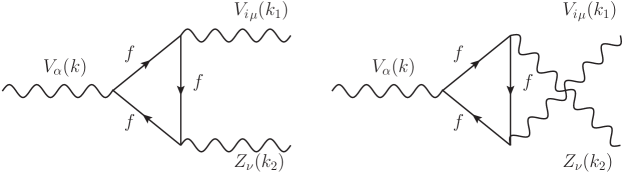
| (44) |
where the four-momenta and correspond to the outgoing and gauge bosons, respectively. The mass factor and the scalar products were included for convenience purpose only. The above amplitude displays explicitly electromagnetic gauge invariance. Assuming the couplings given in Eq. (51), the coefficients can be written in terms of Passarino-Veltman scalar functions as follows
| (45) | |||||
| (46) | |||||
where and , with the fermion electric charge, the fermion color number and the couplings of the gauge boson to the fermions. The sum is over all the charged fermions. Anomaly cancellation requires that . stands for the following two-point scalar functions , , and , while is a three-point scalar function scaled by the mass. It is evident that the coefficients are free of ultraviolet divergences. After the above amplitude is squared and summed (averaged) over polarizations of outgoing (ingoing) particles, we obtain the following decay width
| (47) |
We now concentrate on the decay. The respective amplitude must obey Bose symmetry and can be written as
| (48) |
where and are the four-momenta of the outgoing gauge bosons. The coefficient is
| (49) | |||||
with , , and . The two-point scalar functions and were given above, while the scaled three-point scalar function is . The sum is now over all fermions. Anomaly cancellation requires that . The decay width is given by
| (50) |
We will examine below the behavior of the branching ratios of all the above decays as functions of the symmetry breaking scale and the mixing angle . The results will be discussed in Sec. IV.
III.2 Simplest Littlest Higgs model
In this model the main tree-level decays allowed by kinematics are , , , , , , , , , and . There are no decays into the heavy gauge bosons nor . In the case of the two-body decays, we can readily use the expressions given above, Eqs. (41)-(43), after replacing the respective coupling constants and the extra neutral gauge boson mass. The same method described above was used for the calculation of the three-body decays. As far as the one-loop two-body decays and are concerned, Eqs. (44) -(50) are also valid. We only need to insert the proper coupling constants of the gauge boson to a fermion pair. We have calculated the branching ratios for all these decays as functions of the scale . The results are shown in Sec. IV.
IV Numerical discussion results and experimental perspectives
We now turn to present the numerical results for the branching ratios of the extra neutral gauge boson decays in the previously discussed versions of the little Higgs model. We will first discuss the current constraints on the symmetry breaking scale .
In the original LHM, the bounds on the scale depend on the mixing angles of the gauge sector: and . Such constraints can be obtained from electroweak precision measurements, such as the pole data, low-energy neutrino-nucleon scattering, and measurements of the mass Csaki:2002qg ; Hewett:2002px ; Csaki:2003si ; Gregoire:2003kr ; Chen:2003fm ; Casalbuoni:2003ft ; Marandella:2005wd ; Han:2005dz ; Kilian:2003xt . The largest corrections to electroweak precision observables arise from the heavy gauge bosons Csaki:2002qg . A global fit to experimental data severely constrains the symmetry breaking scale, TeV, for a wide region of values of the mixing parameters Csaki:2002qg . This would require reintroducing fine-tuning to have a light Higgs boson, which would render the model somewhat unattractive. It was suggested however that dangerous corrections to electroweak precision observables could be controlled by tuning the parameters of the model Han:2003wu , which would allow for a less stringent constraint on the scale . In fact, if a suitable assignment of the quantum numbers of the light fermions under the new gauge group is chosen, can be as low as 1-2 TeV in a small region of the parameter space Csaki:2002qg . Another solution requires the introduction of T-parity into the model Low:2004xc , which forbids a triplet VEV and cancels the tree-level contributions to electroweak observables arising from the heavy gauge bosons. In this scenario, the constraint on the scale is significantly weaker than in the original LHM: can be as low as 500 GeV Hubisz:2005tx . For the latest direct bounds on the LHM with T-parity see also Perelstein:2011ds . However, in this model the gauge boson can only decay into a heavy photon plus additional SM particles and so the decays we are interested in are forbidden. As far as the SLHM is concerned, it was argued that the addition of an explicit quartic Higgs coupling yields a region of the parameter space in which the constraints from electroweak precision measurements are naturally satisfied, thereby allowing for a less restrictive bound on . However, the actual constraint on is of the order of TeV as shown in Csaki:2003si , which does not necessarily spoils the model as it does not imply a large amount of fine-tuning: the top partner, which gives the most dangerous corrections to electroweak precision observables, can be relatively light as it can arise at a lower scale than by a suitable election of the model parameters.
We are now ready to discuss the numerical results for the decays of the extra neutral gauge boson.
IV.1 Littlest Higgs model
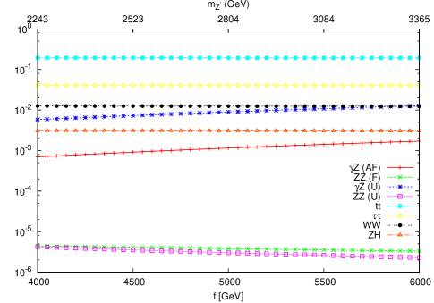
In this model the boson decay widths have a strong dependence on the mixing angle of the gauge sector, namely, . We will first analyze the results for the decays as functions of the mixing angle and for a particular value of . Then we will examine the dependence of the branching ratios on the scale of the symmetry breaking for a fixed value of . In Fig. 2 we show the corresponding results for the branching ratios discussed above as a function of the mixing angle and for TeV, which corresponds to the strongest constraint on the scale . For simplicity we used , although there is little dependence on this parameter. Also, the value GeV is used for the mass of the Higgs boson. We observe that around , the gauge boson decays mainly into a fermion pair. Due to the color number, the decay into a quark pair is slightly dominant over the leptonic one. Apart from the color factor, the branching ratios for the light fermions are almost identical and has little dependence on the fermion mass. The subdominant decays are , , , , , , and . The branching ratios for the last two decays are of similar size and the latter was not included in the plot. Other tree-level decays such as , , , , and exactly vanish when . On the other hand, when is far from , the decay width can be as dominant as the fermion decays. As far as the one-loop decays are concerned, the branching ratio can be as high as the tree-level decays or , but the decay has a very small branching ratio. The former has a branching ratio of the order of while the latter has a rate of about .

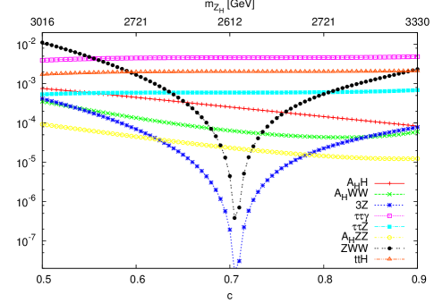
We now set the mixing angle at the value and plot the branching fractions for the decays as functions of the scale , as shown in Fig. 3. Several decay channels vanish in this scenario as commented above due to the vanishing of the couplings involved in the decay amplitude. It is interesting to note that the branching ratio is even larger than the ones for the tree-level decays involving a heavy photon. The latter are suppressed by phase space due to the large value of . However, the decay has a negligible branching ratio and it would hardly have the chance of being detected.
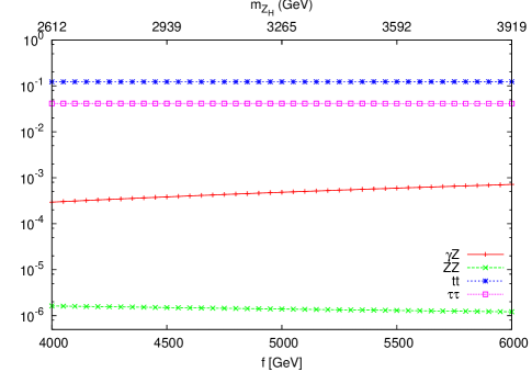
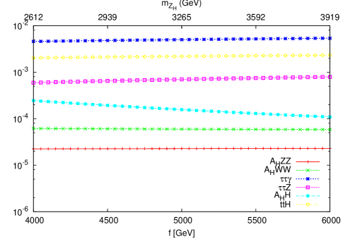
IV.2 Simplest Little Higgs
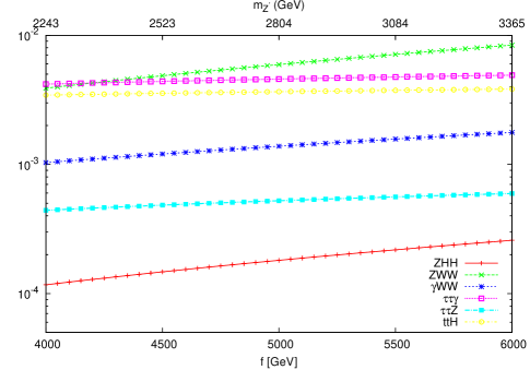
In this model, apart from the symmetry breaking scale , the couplings have no dependence on additional free parameters. The branching ratios for the decays and are shown in Fig. 4 as functions of the symmetry breaking scale in the anomaly-free embedding and also in the universal embedding. The branching ratios for the main decays arising at the tree-level are also shown. We can observe that the boson would decay mainly into a quark-antiquark pair, with a branching ratio larger than the one for the leptonic decays due to the factor arising from the color number. The branching ratios is about one order of magnitude below and other decay channels such as , , and , , , , and have a smaller branching ratio, though they may be at the reach of detection. All these decay channels are always present, in contrast with the case of the LHM, where several decays are absent when . As far as the one-loop decay are concerned, their branching ratios are of the order of in both the anomaly-free and the universal embedding, while the decay has a rate of about in the anomaly-free embedding but is about one order of magnitude larger in the universal embedding. While the branching ratio remains almost unchanged in both the anomaly-free and the universal embeddings, the branching ratio depends strongly on the anomaly cancellation mechanism.
IV.3 Experimental perspectives
Given the recent CDF, ATLAS, and CMS results, we expect conclusive news about the existence of a gauge boson as long as its mass is between 1 and 3 TeV. LHC experiments, by using a total integrated luminosity of 10 fb-1, will be able to discover or rule out a neutral gauge boson with a mass up to 2-3 TeV at 95% C.L. Aaltonen:2011gp ; Chatrchyan:2011wq ; atlascolab . Those experiments have been optimized to look for signals from narrow spin-1 resonances, like our hypothetical heavy neutral gauge boson, decaying into electron or muon pairs. Recently, CDF Aaltonen:2011gp , CMS Chatrchyan:2011wq , and ATLASatlascolab have reported a lower limit on the mass of the order of 1 TeV assuming SM-like couplings to fermions. In such a scenario, the so-called sequential standard model (SSM), ATLAS and CMS have explored the potential discovery of a decaying into leptons, for several values, at , and TeV Diener:2010sy ; Petriello:2008pu .
At the LHC, the production of an extra neutral gauge boson would proceed mainly via the Drell-Yan process Burdman:2002ns ; Han:2003wu ; Han:2005ru . Using the branching ratios obtained above in the LHM and the SLHM, we have calculated the number of events at TeV and an integrated luminosity of fb-1. For comparison purpose we also included the expected number of dilepton events. For the model parameters, we have used the values TeV and . These values correspond to TeV in the LHM and TeV in the SLHM. The results are shown in Tables 1 and 2. Bearing in mind a comparison between our calculations and the published ATLAS and CMS results, we applied the average correction factor value reported in Aad:2009wy ( is the geometrical acceptance and is the reconstructed efficiency for the channel) to the number of expected events.
| LHM | ||
|---|---|---|
| Decay channel | TeV | |
| fb | ||
| fb | ||
| fb | ||
| Anomaly-free Embedding | ||
| Decay channel | TeV | |
| fb | ||
| fb | ||
| fb | ||
| Universal Embedding | ||
| Decay channel | TeV | |
| fb | ||
| fb | ||
It is clear that there are promising expectations for the discovery of an extra neutral gauge boson decaying into a lepton pair, in both the LHM and the SLHM. As soon as the LHC reaches the nominal = 14 TeV energy, it will take a few years to collect 100 fb-1 of integrated luminosity. For TeV and TeV, which are the corresponding values for the chosen value of , the expectations are of the order of a few hundred events in the LHM and a few dozens in the SLHM. These results are similar to those obtained in other models Nath:2010zj ; Langacker:2009su ; Rizzo:2006nw , though they are one or two orders of magnitude smaller than those reported by ATLAS and CMS, using the SSM model. As far as the potential observation of the and decay channels is concerned, LHC experiments have studied the sensitivity to the production of SM diboson events, including the and signals with the gauge boson decaying into a highly energetic lepton pair ( and ) accompanied by an isolated high photon Chatrchyan:2011rr ; Aad:2011tc ; Outschoorn:2010pt ; Aaltonen:2010gy . The -channel production is of special interest due to its sensitivity to the () vertex Larios:2000ni , which is forbidden at tree-level in the SM. From Table 1, we observe that there would be about 14 events, which gives some room for a detailed data analysis. For a heavier , an increase of about one order of magnitude in the integrated luminosity would be necessary to look for this decay process. As for the decay channel, where the final state includes four leptons, it is clear that an experimental signature is not favorable. However, if we consider that the total LHC integrated luminosity will be of the order of fb-1, there is still some chance to observe the decay channel. The results for the detection of these decays channels in the framework of the SLHM depend on the mechanism of anomaly cancellation, which can enhance considerably the branching ratio. While the decays has little chances of being detected, the detection of the decay would depend on the “true“ mechanism of anomaly cancellation. For instance, in the universal embedding there is more chances of detecting the decay. Note that the cross section from production of a gauge boson is also larger in the SLHM with universal embedding as compared to the version with anomaly-free embedding.
In the case of linear colliders Djouadi:2007ik , we have calculated the in both the LHM and the SLHM. For the same and parameter values chosen above, a promising scenario for the discovery of the and decay channels would be an accelerator machine with TeV and an integrated luminosity of the order of 1000 . With these conditions, we obtain approximately 10 events but less than one event. In general, the possible detection of the decays would improve largely for a center-of-mass energy near the resonance. In this respect, the CLIC potential is very promising for detecting several decays of an extra neutral gauge boson with a mass of the order of TeVs.
V Conclusions and outlook
We have calculated the one-loop decays () in the framework of two popular versions of the little Higgs model. Since these decays depend strongly on the mechanism of anomaly cancellation, their study would provide complementary information that could help us to unravel the underlying theory. While the branching ratio for the decay can be as large as in the LHM, the decay has a branching ratio of the order of for 4 TeV. In the SLHM the branching ratio is about in the anomaly free embedding but can be enhanced by about one order of magnitude in the universal embedding. The decay is very suppressed and have branching ratios of the order of in both the anomaly-free and the universal embedding. These class of decays are forbidden in the LHM with T-parity. However, the () decays can be of interest. These decays proceed through triangle diagrams that include two different fermions in the loop (one T-odd and one T-even) and the calculation is more involved. The results for these decays will be presented elsewhere.
We have also discussed the prospects for the experimental observation of the decays at the LHC. While the detection of an extra neutral gauge boson, with a mass of about 3 TeV, decaying into a lepton pair looks very promising in both the LHM and the SLHM, the situation for the decays would be less favorable. In fact, it would be necessary to collect more than 1000 fb-1 of integrated luminosity in order to have few candidate events. The observation of the decay would be even less favorable. As far as the situation in the SLHM is concerned, since the decays are highly dependent on the mechanism of anomaly cancellation, a more detailed knowledge of this mechanism would be necessary to asses the possibility of detection of these decay modes. As far as the prospects at a future collider are concerned, it would be required a center-of-mass energy near the resonance to allow the detection of rare decays of an extra neutral gauge boson, as the ones discussed in this work.
Acknowledgements.
We acknowledge support from Conacyt and SNI (México). Support from VIEP-BUAP is also acknowledged.Appendix A Couplings of the extra neutral gauge boson in little Higgs models
In this appendix we collect all the Feynman rules necessary for our calculation in the unitary gauge. They were taken from Refs. Burdman:2002ns ; Han:2003wu and Han:2005ru .
A.1 Couplings to the light and heavy fermions
The coupling of the extra neutral gauge boson to a fermion pair can be written as
| (51) |
with the usual chirality projectors.
In the LHM, the couplings of the gauge boson to SM fermions are universal and are given by and , where for up (down) type fermions. Although the gauge boson couples to a top quark partner pair, this coupling is very suppressed as it arises up the order of . The same is true for the nondiagonal coupling , which is of the order of . We have neglected those Feynman diagrams mediated by those couplings and have only considered couplings to fermions of the same flavor.
As far as the SLHM is concerned, the couplings of the gauge boson to the fermions depend on the embedding of the heavy fermions. In Table 3 we collect the couplings to SM fermions in both the universal and anomaly-free embeddings, whereas the couplings to heavy fermions are shown in Table 4. On the other hand, the gauge boson couplings to SM fermions are the same as the SM ones but corrected by terms of the order of . The couplings of the boson to heavy fermions are also presented in Table 4.
| Universal | Anomaly-free embedding | |||
|---|---|---|---|---|
| 0 | 0 | |||
| () | ||||
| () | ||||
| couplings | couplings | ||
|---|---|---|---|
| 0 | |||
| , | |||
| , | |||
A.2 Couplings to SM gauge bosons and the Higgs boson
We now present the couplings of the extra neutral gauge boson to the Higgs boson and the SM gauge bosons.
The and couplings, with standing for a neutral gauge boson, can be written as
| (52) | |||||
| (53) |
The Feynman rule for the trilinear gauge boson vertex, with all particles outgoing, is given by
| (54) |
whereas the quartic gauge boson coupling can be written as
| (55) |
The corresponding couplings constants in both the LHM and the SLHM are shown in Table 5.
| LHM () | SLHM () | |
|---|---|---|
| 0 | ||
| 0 |
A.3 Couplings involving other heavy gauge bosons
We first present the couplings involving the heavy photon and the heavy charged gauge boson arising in the LHM. These couplings are necessary for the calculation of various tree-level three-body decays of the extra neutral gauge boson. The Feynman rules for this kind of couplings are given in Eq. (53) through Eq. (55). We present the coupling constants for the LHM in Table 6. Notice that in the framework of the SLHM, the heavy photon is absent and there is no quartic couplings involving the heavy charged gauge boson with the extra neutral gauge boson . Besides, the couplings and vanish.
| LHM | |
|---|---|
Finally, we present some additional couplings necessary for the calculation of the decays in Table 7. Some SM couplings involved in the calculation of the decays of the extra neutral gauge boson receive corrections of the order of but they were neglected from our calculation.
| LHM | |
|---|---|
References
- (1) [ALEPH Collaboration and DELPHI Collaboration and L3 Collaboration and ], arXiv:hep-ex/0511027.
- (2) N. Arkani-Hamed, A. G. Cohen and H. Georgi, Phys. Lett. B 513, 232 (2001) [arXiv:hep-ph/0105239].
- (3) N. Arkani-Hamed, A. G. Cohen, E. Katz and A. E. Nelson, JHEP 0207, 034 (2002) [arXiv:hep-ph/0206021].
- (4) N. Arkani-Hamed, A. G. Cohen, T. Gregoire and J. G. Wacker, JHEP 0208, 020 (2002) [arXiv:hep-ph/0202089].
- (5) N. Arkani-Hamed, A. G. Cohen, E. Katz, A. E. Nelson, T. Gregoire and J. G. Wacker, JHEP 0208, 021 (2002) [arXiv:hep-ph/0206020].
- (6) I. Low, JHEP 0410, 067 (2004) [arXiv:hep-ph/0409025].
- (7) D. E. Kaplan and M. Schmaltz, JHEP 0310, 039 (2003) [arXiv:hep-ph/0302049].
- (8) M. Schmaltz, JHEP 0408, 056 (2004) [arXiv:hep-ph/0407143].
- (9) C. Csaki, J. Hubisz, G. D. Kribs, P. Meade and J. Terning, Phys. Rev. D 67, 115002 (2003) [arXiv:hep-ph/0211124].
- (10) J. L. Hewett, F. J. Petriello and T. G. Rizzo, JHEP 0310, 062 (2003) [arXiv:hep-ph/0211218].
- (11) C. Csaki, J. Hubisz, G. D. Kribs, P. Meade and J. Terning, Phys. Rev. D 68, 035009 (2003) [arXiv:hep-ph/0303236].
- (12) T. Gregoire, D. Tucker-Smith and J. G. Wacker, Phys. Rev. D 69, 115008 (2004) [arXiv:hep-ph/0305275].
- (13) M. C. Chen and S. Dawson, Phys. Rev. D 70, 015003 (2004) [arXiv:hep-ph/0311032].
- (14) R. Casalbuoni, A. Deandrea and M. Oertel, JHEP 0402, 032 (2004) [arXiv:hep-ph/0311038].
- (15) G. Marandella, C. Schappacher and A. Strumia, Phys. Rev. D 72, 035014 (2005) [arXiv:hep-ph/0502096].
- (16) Z. Han and W. Skiba, Phys. Rev. D 72, 035005 (2005) [arXiv:hep-ph/0506206].
- (17) W. Kilian and J. Reuter, Phys. Rev. D 70, 015004 (2004) [arXiv:hep-ph/0311095].
- (18) J. Hubisz, P. Meade, A. Noble and M. Perelstein, JHEP 0601, 135 (2006) [arXiv:hep-ph/0506042].
- (19) G. Burdman, M. Perelstein and A. Pierce, Phys. Rev. Lett. 90, 241802 (2003) [Erratum-ibid. 92, 049903 (2004)] [arXiv:hep-ph/0212228].
- (20) T. Han, H. E. Logan, B. McElrath and L. T. Wang, Phys. Rev. D 67, 095004 (2003) [arXiv:hep-ph/0301040].
- (21) T. Han, H. E. Logan and L. T. Wang, JHEP 0601, 099 (2006) [arXiv:hep-ph/0506313].
- (22) J. Hubisz and P. Meade, Phys. Rev. D 71, 035016 (2005) [arXiv:hep-ph/0411264].
- (23) A. Belyaev, C. R. Chen, K. Tobe and C. P. Yuan, Phys. Rev. D 74, 115020 (2006) [arXiv:hep-ph/0609179].
- (24) A. Freitas and D. Wyler, JHEP 0611, 061 (2006) [arXiv:hep-ph/0609103].
- (25) P. Langacker, Rev. Mod. Phys. 81, 1199 (2009) [arXiv:0801.1345 [hep-ph]].
- (26) J. Erler and P. Langacker, Phys. Rev. Lett. 84, 212 (2000) [arXiv:hep-ph/9910315].
- (27) T. Aaltonen et al. [CDF Collaboration], Phys. Rev. Lett. 99, 171802 (2007) [arXiv:0707.2524 [hep-ex]].
- (28) J. Alcaraz et al. [ALEPH Collaboration and DELPHI Collaboration and L3 Collaboration and ], arXiv:hep-ex/0612034.
- (29) D. Chang, W. Y. Keung and S. C. Lee, Phys. Rev. D 38, 850 (1988).
- (30) M. A. Perez, G. Tavares-Velasco and J. J. Toscano, Phys. Rev. D 69, 115004 (2004) [arXiv:hep-ph/0402156].
- (31) M. Perelstein and Y. H. Qi, Phys. Rev. D 82, 015004 (2010) [arXiv:1003.5725 [hep-ph]].
- (32) A. Flores-Tlalpa, J. Montano, F. Ramirez-Zavaleta, J. J. Toscano, Phys. Rev. D80, 033006 (2009). [arXiv:0906.1852 [hep-ph]].
- (33) A. Flores-Tlalpa, J. Montano, F. Ramirez-Zavaleta, J. J. Toscano, Phys. Rev. D80, 077301 (2009). [arXiv:0908.3728 [hep-ph]].
- (34) D. B. Kaplan and H. Georgi, Phys. Lett. B 136, 183 (1984).
- (35) D. B. Kaplan, H. Georgi and S. Dimopoulos, Phys. Lett. B 136, 187 (1984).
- (36) For a review on little Higgs models and their alternative realizations see: M. Perelstein, Prog. Part. Nucl. Phys. 58, 247 (2007) [arXiv:hep-ph/0512128].
- (37) O. C. W. Kong, arXiv:hep-ph/0307250.
- (38) R. Foot, H. N. Long and T. A. Tran, Phys. Rev. D 50, 34 (1994) [arXiv:hep-ph/9402243].
- (39) J. Boersma and A. Whitbeck, Phys. Rev. D 77, 055012 (2008) [arXiv:0710.4874 [hep-ph]].
- (40) G. Passarino and M. J. G. Veltman, Nucl. Phys. B 160, 151 (1979).
- (41) R. Mertig, M. Bohm and A. Denner, Comput. Phys. Commun. 64, 345 (1991).
- (42) M. Perelstein, J. Shao, [arXiv:1103.3014 [hep-ph]].
- (43) G. ’t Hooft and M. J. G. Veltman, Nucl. Phys. B 153, 365 (1979).
- (44) G. J. van Oldenborgh and J. A. M. Vermaseren, Z. Phys. C 46, 425 (1990).
- (45) T. Hahn, Nucl. Phys. Proc. Suppl. 89, 231 (2000) [arXiv:hep-ph/0005029].
- (46) T. Aaltonen et al. [The CDF Collaboration], Phys. Rev. Lett. 106, 121801 (2011) [arXiv:1101.4578 [hep-ex]].
- (47) S. Chatrchyan et al. [CMS Collaboration], JHEP 1105, 093 (2011) [arXiv:1103.0981 [hep-ex]]. —-2
- (48) The Atlas Collaboration, G. Aad et al., ATLAS sensitivity prospects to and in the decay channels at TeV
- (49) R. Diener, S. Godfrey and T. A. W. Martin, arXiv:1006.2845 [hep-ph].
- (50) F. J. Petriello, S. Quackenbush and K. M. Zurek, Phys. Rev. D 77, 115020 (2008) [arXiv:0803.4005 [hep-ph]].
- (51) G. Aad et al. [The ATLAS Collaboration], arXiv:0901.0512 [hep-ex].
- (52) P. Nath et al., Nucl. Phys. Proc. Suppl. 200-202, 185 (2010) [arXiv:1001.2693 [hep-ph]].
- (53) P. Langacker, arXiv:0911.4294 [hep-ph].
- (54) T. G. Rizzo, arXiv:hep-ph/0610104.
- (55) S. Chatrchyan et al. [CMS Collaboration], arXiv:1105.2758 [hep-ex].
- (56) G. Aad et al. [ATLAS Collaboration], arXiv:1106.1592 [hep-ex].
- (57) V. I. M. Outschoorn [On behalf of the ATLAS Collaboration], arXiv:1011.0164 [hep-ex].
- (58) T. Aaltonen et al. [CDF Collaboration], Phys. Rev. D 82, 031103 (2010) [arXiv:1004.1140 [hep-ex]].
- (59) F. Larios, M. A. Perez, G. Tavares-Velasco and J. J. Toscano, Phys. Rev. D 63, 113014 (2001) [arXiv:hep-ph/0012180].
- (60) G. Aarons et al. [ILC Collaboration], arXiv:0709.1893 [hep-ph].