Quantum entanglement in random physical states
Abstract
Most states in the Hilbert space are maximally entangled. This fact has proven useful to investigate – among other things – the foundations of statistical mechanics. Unfortunately, most states in the Hilbert space of a quantum many-body system are not physically accessible. We define physical ensembles of states acting on random factorized states by a circuit of length of random and independent unitaries with local support. We study the typicality of entanglement by means of the purity of the reduced state. We find that for a time , the typical purity obeys the area law. Thus, the upper bounds for area law are actually saturated, on average, with a variance that goes to zero for large systems. Similarly, we prove that by means of local evolution a subsystem of linear dimensions is typically entangled with a volume law when the time scales with the size of the subsystem. Moreover, we show that for large values of the reduced state becomes very close to the completely mixed state.
Introduction.— Entanglement is the defining characteristic of quantum mechanics: it is a key ingredient in quantum information processingent-qip , quantum many-body theory amico , and the description of novel quantum phases of matter topentropy . More recently, quantum entanglement has shed new light on the foundations of statistical mechanics, and the processes of equilibration and thermalization. The idea consists in the fact that even with unitary evolution, if the entanglement is large enough, the expectation values of local observables are typically close to those of the thermal state qterm ; Tasaki (1998); Popescu et al. (2006). It has been shown that such typicality is related to the volume law for the entanglement in random states Popescu et al. (2006). The problem with this approach is that random states are not physical because they are not accessible in nature. Indeed, one needs a doubly exponential time in the system size to access all the states of the Hilbert space. For this reason, some authors have argued that the Hilbert space is an illusion verstraete .
Nevertheless, physical states do thermalize, as has been shown in experiments with cold atoms, theoretical models and numerical simulations thermquench ; rigol ; Cramer et al. (2008), or show typicality in the expectation value of local observables garnerone . Does this mean that the mechanism for thermalization is not entanglement? There are several examples of physical relevance showing that when evolution time scales with the size of the system, the state is entangled with a volume law cc ; eisert . Can thus we prove any statement about the typicality of such situations?
In this Letter, we propose to answer the following question: how much are typical physical states entangled? We adopt the 2-Renyi entropy as a quantum entanglement quantifier renyi as opposed to von Neumann Entanglement Entropy (EE). While from the technical point of view this choice allows a drastic simplification of the theoretical treatment, on physical grounds, we expect all the scaling results for typical physical states presented in this Letter to be fulfilled by EE as well any other sound quantum entanglement measure.
To this end, we define an ensemble of physical states in this way: pick a product state of a multipartite system, then act with independent random unitaries, each of them compatible with some locality structure, e.g., supported on edges of a graph. This mimics the continuous evolution generated over a time by a local (time dependent) Hamiltonian and are amenable to an elegant analytical treatment. Indeed, by applying the group theoretic techniques of Ref. entpower , we can compute the ensemble average and variance of the Renyi entropy of a subregion with boundary of size . The result is that, typically, for we obtain an area law that is an entanglement , while for scaling as the linear size of the system the average purity shows a volume law. Moreover, we show that fluctuations are small, and that there is measure concentration around the average value. As a final result, we show that for , the subsystem typically reaches the completely mixed state.
Note that the upper bounds to entanglement laws that incorporate the locality of the interactions are known. Using the technique of the Lieb-Robinson bounds, one can prove that entanglement that can be produced in a subsystem by evolving for a time is upper bounded by a quantity scaling with . Here is limit speed for the interactions in the system lrb . In other words, for the area law for the entanglement is an upper bound, while the volume law is an upper bound for . These upper bounds have been proven very useful, e.g., in the context of simulability of quantum many-body systems or the understanding of topological order. However, these are just upper bounds and they deal with an extremal case. It could be the case that most Hamiltonians are very weakly entangling. Therefore one wonders how typical area and volume laws are. Are these upper bounds saturated on average and how strong are the fluctuations around the average? The results of this Letter say that almost every local evolution entangles the subsystem with a scaling law .
A second motivation is found in the context of unitary designs harrow . Known results scale with some polynomial of the total number of degrees of freedom harrow ; recent . In this Letter, we focus on the statistics of observables of a reduced system, and the asymptotic results scale with the size of the reduced system.
Statistical ensemble of physical states.— We start by defining the ensembles ; henceforth we will refer to the elements of these ensembles as the physical states. Let be a set of vertices endowed with a probability measure with . To each of the vertices we associate a local dimensional Hilbert space . The total Hilbert space is thus , or the space of qudits. A completely factorized state in has the form ; let be its density matrix. The statistical ensembles of quantum states are constructed in the following way: We first draw a subset according to the measure and then we draw a unitary according to a chosen measure . Then we define This, ensemble can be generalized to the iterated by considering unitaries of the form where the ’s (’s are drawn according the product probability ( at each tick of the clock a new independent set ’s and a unitary are picked. In this ensemble, we can compute the statistical moments of any Hermitian operator. It turns out that by varying over the , one can pick all the possible factorized ’s so that the dependence can be in fact dropped.
Subsystem purity.— We now examine the typical entanglement in the statistical ensembles Let us consider a bipartition in the system: , where with obvious notation. We take a state and consider the reduced density matrix . In order to evaluate the entanglement of we compute the purity and thus the Renyi entropy . To compute this trace we use the well-known fact that the trace over the square of every operator can be computed as the trace of two tensored copies of that operator times the swap operator. Indeed, defining and considering the order 2 shift operator (swap) on , we have where by is the order shift operator in the space and is given by We can now consider different concrete ensembles. As a basic model, let us consider the case in which there is a just as single edge: the system consists of two sites and connected by an edge so that the Hilbert space is of dimensions . The probability distribution is the trivial and we pick the unitaries with the Haar measure: . Notice that in this case, the ”locality” does not play any particular role. There is just one edge so the unitaries are the unitaries over the whole . Following Ref.entpower , one can exploit the group theoretic structure of the ensemble to compute average and statistical moments of operators. The average of an operator over a group action is indeed the weighted sum of projectors onto the IRreps of the representation of that group. A direct calculation (see supplementary material) shows that For very large , we approximate the completely mixed state. Since the purity is a positive definite quantity that is going to zero in the thermodynamic limit, in the limit for the large system the fluctuations are also very small. Notice that this result reproduces what we know: a random state in the whole Hilbert space is typically very entangled.
Propagation of typical entanglement.— The main goal of this paper is to explore what is the typicality of entanglement when there are some local conditions on how the ensembles of states are constructed. The local conditions are implemented by acting times with random local quantum circuits. We show that the loss of purity in a subsystem propagates, in average, within a length within the bulk of . In this way, we can show that, in average, the entanglement for follows the area law, and for a generic it follows . Moreover, we show that the variance of the distribution of entanglements is very small: the average entanglement is typical. We can then conclude that the laws that determine upper bounds for the entanglement actually also determine the typical situation. In order to obtain this kind of propagation result, we will exploit a result on the algebra of the permutations () defined above. Let us start by defining the superoperator that averages over the unitaries , that is, Notice that when is the Haar measure, the s are projection superoperators; in the rest of the letter we will focus on this case. Then we can evaluate the average purity as
| (1) |
where is a self-dual (Hermitian) superoperator. As a far as the purity calculations are concerned this superoperator completely characterizes the ensembles . Indeed, it is now easy to see that –in view of the statistical independence of each iteration– the average purity for the iterated ensemble is given by the expression (1) with replaced by In order to understand the spectral properties of , observe that: Since we then see that whence the eigenvalues of are bounded in modulus by one and the highest one is . One can then write where and denotes the projection of onto the eigenvalue eigenspace of For this quantity goes to the limite value while the convergence rate is dictated the second highest eigenvalue of hsz2 .
One of the key steps to obtain the results of this Letter is to realize that the ’s superoperators can be regarded as maps on the -dimensional space spanned by the ’s () into itself (instead of maps of the -dimensional into itself). For example, if i.e., an edge and is any subset of a calculation similar to the above leads to
| (2) |
The edge ’s have low-dimensional invariant subspaces of permutations, e.g., in a chain topology the span of the ’s associated with connected ’s is invariant. This remark along with the fact that for product states, allows for drastic simplifications in the evaluation of the average purity of The content of Eq.(2) is that ’ has a non trivial action only if the edge straddles the boundary between the system and .
As an example, let us show how the algebra (2) simplifies the calculation of the average purity for the single edge model. The subsistem is just one site and therefore and . Moreover, and . Finally we get . In the case of qubits, and . It is also possible to compute the variance by generalizing the group averages to higher power of the density operator to obtain . A systematic treatment is to be found in hsz2 .
At this point, we consider a system with a notion of locality, so that it makes sense how average entanglement propagates. To this aim, we define the -random edge model on a graph where is the set of the nodes and the set of the edges. We define a flat probability distribution on the edges of the graph : if and zero otherwise. Then we pick the unitaries on the edges with the Haar measure: . We call the subset of edges that have nonnull intersection with both and . The probability of an edge to belong to is thus . We are interested in the thermodynamic situations where . Using Eq.(2) we get
| (3) |
where is an edge of the graph. One can see that only the terms in Eq.(3) that live across the boundary will decrease the purity of the subsystem. Moreover, the support of is now on graphs with locally modified boundaries. For is then easy to find the average purity: From Eq.(3) we see that every application of transforms the subset into a superposition of and so that at any successive iteration the boundary of the new subset changes and its boundary length may change. The iteration for scaling with the linear size of the system gives the results (see supplementary material) . Therefore the average Renyi entropy of the ensemble is . In terms of the average entangling power entpower , one gets In other words, the average Renyi entropy for the random edge model of the th iteration is lower bounded by times the fraction of vertices in the boundary of the region times the average entangling power of an edge unitary, showing a linear increase of entropy in time, or, in other words, the entanglement is propagating into the bulk of . Moreover, one can compute variances of and show that hsz2 . This in turn implies measure concentration (typicality) in the thermodynamic limit . So a random circuit model of this type can reproduce the Haar measure for the statistics of observables on the reduces system, as scales with the subsystem size.
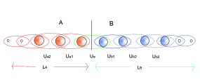
The linear chain.— We now move to the case corresponding to a time dependent Hamiltonian that is the sum of local terms. In this model, the unitaries act on all the edges of the graph The probability distribution is thus for and zero otherwise. For the sake of simplicity in the following, we will consider the case of the graph being a bipartite chain of length . Extensions to higher dimensional geometries will be presented in hsz2 ). We will label by the unitary acting on the edge straddling the bipartition, while we will use the labels for the unitaries that act in the bulk of respectively (see Fig.1). We label the sites of the chain as . Since the unitary is a product of all the edge unitaries, we need to specify in which order they act. In the following, the unitary will always denote the product over all the edges in with the order given by the permutation , so is the ordered product over local two-qudit unitaries. This corresponds to the (time ordered) infinitesimal evolution with a local Hamiltonian, where gives the time ordering: . At this point we construct the set with measure . This ensemble approximates all the states that can be evolved from a factorized state with a local Hamiltonian acting for an infinitesimal amount of time. By iteration, we obtain the time evolution for a finite time Here, we consider all the possible ordered sequences of unitaries by taking, a each time step, a permutation of the edges uniformly at random. This ensemble approximates all the states that can be reached in time by the evolutions originated by all the possible time-dependent Hamiltonians on a graph. The ensemble thus only depends on the number of iterations (the ”time”) and the graph . The loss of purity due to the action of the unitaries depends on their order. Thus, in order to find an upper bound to the average purity, we consider the ordering that gives the minimum loss of purity. As increases, nodes at distance from the boundary participate in the averaging calculation. A lengthy calculation shows that the purity gets a factor for every node participating in the average and we find (see supplementary material) . Summing the series for for large values of one finds . Recall that this equation, in view of the choice of the corresponding to the with the least entangling power, is an upper bound for the purity in The exponential decay of the purity in is due to the fact that all the qudits at distance from the edge are getting mixed. Since average Renyi entropy is we have the lower bound
| (4) |
(Last approximation holds for large ). Eq. (4) for implies a) a volume law for the entanglement scaling b) typicality: a nearly minimal value of the average of purity (in view of the Markov inequality), forces also the fluctuations around this average to be small. For one has no longer a linear increase of entanglement with time but observes a saturation. This type of behavior has been found in examples of entanglement dynamics after a quench using CFT techniques Calabrese (2006); cc ; recent .
To study the limit of average purity for we first notice that the chain superoperator is a (-ordered) product of (non-commuting) projections . This implies again this means that all the eigenvalues of are smaller in modulus than and therefore asymptotically just fixed points e.g., contribution to survives. If now one assumes that the symmetric combination is the only relevant fixed point one finds . We have checked this result by numerical simulations hsz2 for the least and most entangling ’s but we conjecture it to hold true for all orderings and besides the one-dimensional chain scenario. For large one has that in turn for shows that the asymptotic purity differs from that of the totally mixed state for terms of order Finally, if this implies that the vast majority of the states in once reduced to are close in -norm to the maximally mixed state.
Conclusions.— We investigated the typical entanglement in physical states. To this end, we defined statistical ensembles of physical states by considering product states on a multipartite system and evolving them with independent stochastic local gates. Ensemble averages can be computed by introducing suitable superoperators and using group-theoretic tools as in entpower . We would like also to stress that althoughin this Letter we used purity to quantify the entanglement, this method extends in a straightforward way to general -Renyi entropy by natural modifications of superoperator and permutation in Eq.(1) hsz2 . Assuming now that one is allowed to perform an analytic continuation in the limit , our results apply also for the von Neumann Entanglement Entropy. States that are obtained by local evolution for a constant O(1) time have a typical entanglement given by the area law. While the area law was known to hold as an upper bound, we have shown that it is indeed typical. On the other hand, states that are obtained by evolution for a time scaling with the size of the system are shown to almost always obey the volume law for entanglement like typical (Haar) random states do. At this point, we may speculate as to whether this result implies local thermalization for physical states.
Acknowledgments.— We thank M.P. Müller for useful discussions. Research at Perimeter Institute for Theoretical Physics is supported in part by the Government of Canada through NSERC and by the Province of Ontario through MRI. PZ acknowledges support from NSF grants PHY-803304 and PHY-0969969. This research is partially supported by the ARO MURI grant W911NF-11-1-0268.
References
- (1) R. Horodecki, P. Horodecki, M. Horodecki, and K. Horodecki, Rev. Mod. Phys. 81, 865 (2009)
- (2) Luigi Amico, Rosario Fazio, Andreas Osterloh, Vlatko Vedral, Rev. Mod. Phys. 80, 517 (2008)
- (3) A. Hamma, R. Ionicioiu, and P. Zanardi, Phys. Lett. A 337, 22 (2005); A. Kitaev and J. Preskill, Phys. Rev. Lett. 96, 110404 (2006); M. Levin and X.-G. Wen, Phys. Rev. Lett. 96, 110405 (2006).
- Tasaki (1998) H. Tasaki, Phys. Rev. Lett. 80, 1373 (1998; S. Goldstein, J. Leibowitz, R. Tumulka, and N. Zanghí, Phys. Rev. Lett. 96, 050403 (2006); P. Reimann, Phys. Rev. Lett. 99, 160404 (2007).
- (5) J. Gemmer, M. Michel, and G. Mahler, Quantum Thermodynamics, Springer (2005).
- Popescu et al. (2006) S. Popescu, A. J. Short, and A. Winter, Nature Physics 2, 754 (2006); N. Linden, S. Popescu, A. J. Short, and A. Winter, Phys. Rev. E79, 061103 (2009).
- (7) David Poulin, Angie Qarry, R. D. Somma, Frank Verstraete, Phys. Rev. Lett. 106, 170501(2011)
- (8) M. Rigol, V. Dunjko, and M. Olshanii, Nature 452, 854 (2008)
- (9) M. Cramer, C.M. Dawson, J. Eisert, and T.J. Osborne, Phys. Rev. Lett. 100, 030602 (2008)
- Cramer et al. (2008) M. Cramer, A. Flesch, I. P. McCulloch, U. Schollwöck, and J. Eisert, Phys. Rev. Lett. 101, 063001 (2008)
- (11) S. Garnerone, T. R. de Oliveira, P. Zanardi, Phys. Rev. A81, 032336 (2010); S. Garnerone, T. R. de Oliveira, S. Haas, P. Zanardi, Phys. Rev. A 82, 052312 (2010).
- (12) P. Calabrese and J. Cardy, J. Stat. Mech. P04010 (2005); J. Stat. Mech. P10004 (2007)
- (13) M. Cramer, C.M. Dawson, J. Eisert, T.J. Osborne, Phys. Rev. Lett. 100, 030602 (2008); M. Cramer, J. Eisert, New J. Phys. 12, 055020 (2010)
- (14) H. Ju, A.B. Kallin, P. Fendley, M.B. Hastings, and R.G. Melko, Phys. Rev. B 85, 165121 (2012); S. V. Isakov et al, Nature Physics 7, 772 (2011); M. B. Hastings, I. Gonzalez, A.B. Kallin, and R.G. Melko, Phys. Rev. Lett. 104, 157201 (2010); S.T. Flammia, A. Hamma, T.L. Hughes, and X.G. Wen, Phys. Rev. Lett. 103, 261601 (2009)
- (15) P. Zanardi, C. Zalka, and L. Faoro, Phys. Rev. A62, 030301 (2000).
- (16) S. Bravyi, M.B. Hastings, and F. Verstraete, Phys. Rev. Lett. 97, 050401 (2006); J. Eisert and T.J. Osborne, Phys. Rev. Lett. 97, 150404 (2006).
- (17) J. Eisert, M. Cramer, and M.B. Plenio, Rev. Mod. Phys. 82, 277 (2010)
- (18) A. H. Harrow, R. Low, Comm. Math. Phys. 291, 257 (2009)
- (19) L. Masanes, A. J. Roncaglia, A. Acin, arXiv:1108.0374; Vinayak, M. Znidaric arXiv:1107.6035; F. G.S.L. Brandão et al., arXiv:1108.2985;
- (20) A. Hamma, S. Santra, and P. Zanardi, arXiv:1204.0288.
- Calabrese (2006) P. Calabrese and J. Cardy, Phys. Rev. Lett. 96, 136801 (2006)
I Supplementary Material
I.1 Single edge
Let us show the detailed calculation of the average purity for the single edge model. In this case, the IRreps are carried by the totally symmetric () and totally antisymmetric () subspaces of . The average is given by . After the integration we get since is supported only in the totally symmetric subspace whose dimension is and . The projector onto the totally symmetric space has the form and we finally get In entpower2 it was defined the average entangling power as the average entanglement one attains from a factorized bipartite state by averaging over the unitaries in the whole space with the Haar measure. With this definition, [see Eq. (5) inentpower2 ].
I.2 Iteration to in the Random Edge Model
To understand the structure of it is instructive to consider explicitly the case. Iterating (3) and computing the purity using (1) note we find where we have used . This is true e.g. if every vertex has degree . The calculation easily extends to the case and thus one finds .
I.3 Iteration to for the linear chain
Let us first show what is the sequence that lower bounds the amount of average entanglement produced. We can see that, for , acting in and after having acted on the edge does not change the purity, so a sequence of the type results in a minimal loss of purity. Moreover, the order of the unitaries inside and also counts. From the iteration of the algebra Eq.(2) we can see that if we pick the ordering in which we first act near the boundary and proceed towards the outer parts of the chain: where and we will get the lowest possible powers of and correspondingly the least decrease of purity. As increases, the difference between different orderings is attenuated and for very large values of it can also be neglected. We will anyway always consider the worst case scenario of ordering which corresponds to the minimal decrease of purity.
Now we want to show how the algebra Eq.(2) propagates the average entanglement in the linear chain. The action of the superoperator in the linear chain model is more complicated because now is not just the support of one unitary, but it contains the ordered product of all the edges. In particular, notice that now is not hermitean. Using Eq.(2) multiple times we find: for , . Where we used the notation and . At the second iteration , we get . We can see that nodes at distance from the boundary enter the expression. Each in the expression for gives a when we take the scalar product with . So we find . It is important to understand how the interactions propagate with . A somewhat lengthy calculation shows that as increases, nodes at distance from the edge participate to the averaging procedure and for every node that participates we pick a power for the base . For calculation gives .
References
- (1) P. Zanardi, C. Zalka, and L. Faoro, Phys. Rev. A62, 030301 (2000)
- (2) Notice that always for product states, which shows why the initial choice of the product state is irrelevant.