Mixtures of conditional Gaussian scale mixtures
applied to multiscale image representations

Abstract

We present a probabilistic model for natural images which is based on Gaussian scale mixtures and a simple multiscale representation. In contrast to the dominant approach to modeling whole images focusing on Markov random fields, we formulate our model in terms of a directed graphical model. We show that it is able to generate images with interesting higher-order correlations when trained on natural images or samples from an occlusion based model. More importantly, the directed model enables us to perform a principled evaluation. While it is easy to generate visually appealing images, we demonstrate that our model also yields the best performance reported to date when evaluated with respect to the cross-entropy rate, a measure tightly linked to the average log-likelihood.

1 Introduction

Probabilistic models of natural images are used in many fields related to vision. In computational neuroscience, they are used as a means to understand the structure of the input to which biological vision systems have adapted and as a basis for normative theories of how those inputs are optimally processed [1]. In computer science, they are used as priors in applications such as image denoising [2], compression [3], or reconstruction [4] and to learn image representations that can be used in object recognition tasks [5]. The more abstract goal common to these efforts is to capture the statistics of natural images.

The dominant approach to modeling whole images has been to use undirected graphical models (or Markov random fields). This is despite the fact that directed models possess many advantages over undirected models [4, 6]. In particular, sampling as well as exact maximum likelihood learning can often be performed efficiently in directed models while presenting a major challenge with most undirected models. Another problem faced by undirected models is the question of how to evaluate them. Ideally, we would like to quantify the amount of second- and higher-order correlations captured by a model. For stochastic processes, this can be done by calculating the cross-entropy rate between the learned distribution and the true distribution, which represents the analogue to the negative log-likelihood for patch-based models. However, the cross-entropy rate is typically difficult to estimate in undirected models so that these models are often evaluated only with respect to surrogate measures such as performance in supervised tasks, simple statistics computed from approximate model samples or simply the samples’ visual appearance. These measures, however, are less objective and hence need to be used with great caution. A large lookup table storing examples from the training set, for example, will reproduce samples which are indistinguishable from true samples for the human eye and yield near to perfect performance when evaluated based on simple statistics. Yet this model is heavily overfit to a few examples of natural images. Effectively, it assigns zero probability to images that have not been stored in the lookup table and would thus perform miserably if evaluated based on the cross-entropy rate. In fact, the cross-entropy rate does not leave any room for prestidigitation and therefore provides a crucial basis for the comparison of natural image models.

Following the directed approach, we will demonstrate here that a directed model applied to multi-scale representations of natural images is able to learn and reproduce interesting higher-order correlations. We use multiscale representations to separate the coarser components of an image from its details, thereby facilitating the modeling of both very global and very local image structure. The particular choice of our representation makes it possible to still evaluate the cross-entropy rate and to further investigate the scale-invariance of natural images.

2 A directed model for natural images

Figure 1: Left: A conditional model with a twenty-four pixel causal neighborhood. Sampling is performed by shifting the causal neighborhood from left to right and from top to bottom. Right: Graphical model representation with only four pixels in the causal neighborhood. The parents of a pixel are constrained to pixels which are above of it or in the same row and left of it.

One way to model the statistics of arbitrarily large images is to use a directed model in which the parents of a node are constrained to pixels which are left or above of it (Figure 1). A set of parents fulfilling this constraint is also called a causal neighborhood [6] and the resulting model a causal random field. Note that a pixel will still depend on neighbors in all directions, that is, the causal neighborhood assumption puts only mild constraints on the size or shape of a pixel’s Markov blanket. An advantage of the directed model is that it allows us to easily decompose the distribution defined over images or, more generally, a two-dimensional stochastic process $X$ indexed by $x,y$, into a product of conditional distributions:

$$P(X)=\prod_{x,y}P(X_{x,y}\mid\mathrm{Pa}_{x,y}),$$ (1)

where $\mathrm{Pa}_{x,y}$ refers to the causal neighborhood of pixel $X_{x,y}$. Consequently, performing maximum likelihood learning by maximizing the log-likelihood of the model can be done by optimizing a set of conditional probability distributions. To sample an image from the model, the causal neighborhood is shifted from top to bottom and from left to right, filling an image row by row. This procedure requires that the top rows and left columns of the image are initialized to provide input to the conditional distributions. Generally, these cannot be filled with pixels drawn from the distribution of the model. As a consequence, only after the procedure has generated a few rows and converged to the model’s distribution will it generate the desired samples.

2.1 Mixture of conditional Gaussian scale mixtures

To complete the model, the conditional distribution of each pixel given its causal neighborhood has to be specified. We will assume stationarity (or shift-invariance), so that this task reduces to the specification of a single conditional distribution. A family of distributions which has repeatedly been shown to contain suitable building blocks for modeling the statistics of natural images is given by Gaussian scale mixtures (GSMs) [7, 8],

$$p(x)=\int\varphi(z)\mathcal{N}(x;\mu,zC)dz,$$ (2)

where $\mathcal{N}(x;\mu,zC)$ is a multivariate Gaussian density with mean $\mu$ and covariance $zC$ and $\varphi(z)$ is some univariate density over scales $z$. Mixture models and Markov random fields based on GSMs have been successfully applied to denoising tasks [2, 9]. When used in the directed setting also employed here, GSMs have been shown to yield highly improved estimates of the multi-information rate of natural images [6].

Here we use the conditional distribution of a mixture of GSMs to model the distribution of a pixel given its causal neighborhood. We restrict ourselves to mixtures of finite GSMs, that is, GSMs with a finite number of scales, and to mixtures in which each component and scale has equal a priori weight. Additionally, we assume that each GSM has mean zero. If variables $x$ and $y$ are modeled jointly with a mixture of GSMs, the conditional distribution of $y$ given $x$ can be written as

$$p(y\mid x) =\sum_{c,s}\underbrace{p(c,s\mid x)}_{\text{gate}}\underbrace{p(y\mid x,c,s)}_{\text{expert}},$$ (3)

where $c,s$ run over mixture components and scales, respectively. From this formulation it is clear that the conditional distribution falls into the mixtures of experts framework [10]. In this framework, the predictions of multiple predictors—the experts—are mixed according to weights which are computed locally by so called gates. For the mixture of GSMs with the constraints above we have

$$p(c,s\mid x) \propto|\lambda_{cs}K_{c}|^{\frac{1}{2}}\exp(-\frac{1}{2}x^{\top}\lambda_{cs}K_{c}x),$$ (4)

$$p(y\mid x,c,s) \propto\exp(-\frac{1}{2}(y-A_{c}x)^{\top}\lambda_{cs}M_{c}(y-A_{c}x)),$$ (5)

where $M_{c}$ and $K_{c}$ are positive definite matrices and $\lambda_{cs}$ are positive. The gates pick an expert based on the covariance structure and scale of the input variables $x$. Each expert is just a Gaussian with a linearly predicted mean. The conditional distribution can equivalently be described as a mixture of conditional Gaussian scale mixtures (MCGSM), because conditioned on $c$ the conditional distribution is again a GSM.

2.2 A simple multiscale representation

Figure 2: Starting with a regular grey-scale image, the pixels are grouped into two by two pixels. Each group is then transformed using the Haar wavelet basis on the right. The resulting basis coefficients can be interpreted as channels of an image of which one channel is essentially the original image at a coarser scale (lower resolution). Just as in the original representation, we can define a directed model and causal neighborhoods for the superpixel representation. If the low-resolution image is given, the prediction of a pixel can be based on information from anywhere in the low-resolution image (not just a causal neighborhood) without losing the ability to efficiently sample or optimize the parameters of the model.

To facilitate the modeling of global as well as local structure, we introduce a multiscale representation which allows us to model an image at multiple resolutions. We start by transforming an image into a representation consisting of a low-resolution version of the image and a separate representation for its details. This is achieved by grouping the image into patches of two by two pixels and transforming each patch using a Haar wavelet basis. One component of the Haar wavelet basis essentially performs a block-average on the image, the result of which forms the low-resolution part of the representation. The three remaining coefficients encode the more detailed structure (Figure 2).

The transformed image can be viewed as an image with multiple channels where each set of basis coefficients corresponds to one channel. We will call the multi-channel pixels in the new representation superpixels. Just as we would model RGB images, we can model images in this new representation with the MCGSM by predicting all channels of a superpixel at once.

If we assume further that the low-resolution channel of the image is given, we can base our predictions on an arbitrary set of pixels from the low-resolution image without losing the ability to efficiently perform maximum likelihood learning or to sample from the model. This can be seen as follows. Just like the transformation of four pixels using the Haar wavelet basis, the transformation between the two representations, $\phi$, is a linear transformation with a Jacobian determinant of 1. If $\phi(X^{0})=(Y^{1},X^{1})$ is the superpixel representation of an image $X^{0}$, consisting of a low-resolution part $X^{1}$ and a high-resolution part $Y^{1}$, we have

$$P(X^{0})=P(\phi(X^{0}))\underbrace{|\det D\phi(X^{0})|^{-1}}_{=1}=P(Y^{1},X^{1})=P(Y^{1}\mid X^{1})P(X^{1}).$$ (6)

Each factor on the right-hand side again factors into a product of the form of Equation 1. Sampling an image is achieved by first sampling a low-resolution image $X^{1}$ and then conditionally sampling $Y^{1}$. Every variable that has already been sampled can be used to sample and predict the remaining variables. Maximizing the log-likelihood amounts to maximizing the logarithm of the two factors on the right-hand side.

By recursively applying the transformation to the low-resolution image of the representation, we end up with a pyramid of images where each level contains the high-resolution information that completes the image represented by the levels above of it. At the top of the pyramid, that is, the lowest resolution, we will again model the image with an MCGSM, so that after applying the transformation $M$ times we are using $M+1$ MCGSMs.

2.3 Model evaluation

A principled way to evaluate a model approximating a stochastic process $X$ is to use the model to estimate the true distribution’s multi-information rate (MIR),

$$I_{\infty}[X]=\lim_{N\rightarrow\infty}\frac{1}{N}\sum_{n=1}^{N}H[X_{n}]-H[X_{1},...,X_{N}],$$ (7)

where $H$ denotes the (differential) entropy. A related measure is the entropy rate,

$$H_{\infty}[X]=\lim_{N\rightarrow\infty}\frac{1}{N}H[X_{1},...,X_{N}].$$ (8)

For a strictly stationary Markov process, one can show that these quantities reduce to [6, 11]

$$H_{\infty}[X] =H[X_{N}\mid\mathrm{Pa}_{N}],$$ (9)

$$I_{\infty}[X] =H[X_{1}]-H[X_{N}\mid\mathrm{Pa}_{N}],$$ (10)

for some $N$. By replacing the entropy rate with the cross-entropy rate—a limit of cross-entropies instead of entropies—we obtain a lower bound on the true MIR. We will call this lower bound the cross-MIR in the following. If the assumption of stationarity or the Markov assumption is not met by the true distribution, the cross-MIR will still be a lower bound but will become more loose [6]. The difference between the true MIR and the cross-MIR is the Kullback-Leibler divergence between the true distribution and the model distribution. Therefore, the better the approximation of the model to the true distribution, the larger the cross-MIR.

Maximizing the cross-MIR by minimizing the cross-entropy rate is the same as maximizing the average log-likelihood. The MIR quantifies the amount of second- and higher-order correlations of a stochastic process. Similar to the likelihood, the cross-MIR can be said to capture the amount of correlations learned by the model. In addition, it has the advantage of being easier to interpret than the likelihood or the cross-entropy rate, as it is always non-negative and invariant under multiplication of the stochastic process with a constant factor. An independent white noise process has a MIR of zero. In the stationary case, evaluating the cross-MIR amounts to calculating one marginal entropy and one conditional cross-entropy (see Equation 10).

Since the superpixel representation is just a linear transformation of the original image, we can evaluate the entropy rate also for the multiscale model. Using the fact that the transformation has a Jacobian determinant of 1, the following relationship holds for the entropy and cross-entropy rates:

$$H_{\infty}[X^{0}]=\frac{1}{4}H_{\infty}[Y^{1}\mid X^{1}]+\frac{1}{4}H_{\infty}[X^{1}].$$ (11)

The factor $\frac{1}{4}$ is due to the superpixel representation having four channels. This result readily generalizes to the multiscale representation by recursively applying it to the right term on the right-hand side of Equation 11. This means that in order to estimate the cross-entropy rate of our model, we only need to compute the cross-entropy rates at the different scales and form a weighted average.

3 Experiments

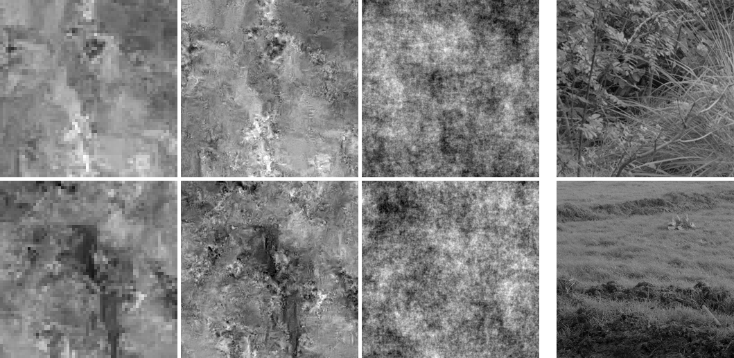
Figure 3: The first column shows a sample from the MCGSM at the largest scale. The second column shows a sample from our model at a smaller scale, conditionally sampled with respect to the sample on the left. The third column shows the same samples with all higher-order correlations destroyed but the autorocorrelation function left intact. The right most column shows examples of images from the training set, that is, the van Hateren dataset [12].

We extracted training data at four different scales from log-transformed images taken from the van Hateren dataset [12]. In all experiments, we used $200000$ training examples of inputs and outputs. To model the coarsest scale, we used an MCGSM with a causal neighborhood corresponding to the upper half of a $7\times 7$ neighborhood surrounding the predicted pixel (as in Figure 1). For the finer scales, we trained three MCGSMs with $3\times 3$ superpixel neighborhoods (as in Figure 2). All models consisted of 8 components with 4 scales each. The parameters were trained using the BFGS quasi-Newton method [13]. For faster convergence, we initialized the conditional models with parameters from mixtures of GSMs trained on the joint distribution of inputs and outputs using expectation maximization. Initializing the models in this way also led to more stable as well as slightly better results. At each scale, we initialized the boundaries of the image with small random white noise and sampled an image large enough for the sampling procedure to reach convergence to the model’s stationary distribution. We then extracted the center part of the image and used it as the input to the model at the next scale.

Samples from the model are shown in Figure 3. We find that the model is able to generate images with some interesting properties which cannot be found in other models of natural images. Perhaps the most striking property of the sampled images is the heterogeneity expressed in the combination of flat image regions with regions of high variance as it can also be observed in true natural images.

By destroying the higher-order correlations but keeping the second-order correlations, we get the familiar pink noise images (Figure 3). This shows that the model faithfully reproduces the autocorrelation function of natural images, and that the characteristic features of the sampled images are due to higher-order correlations learned by the model. The higher-order correlations were removed by replacing the phase spectrum of the image with a random phase spectrum obtained from a white noise image but keeping the sample’s amplitude spectrum. For stationary processes, the amplitude spectrum defines the autocorrelation function of an image and vice versa.

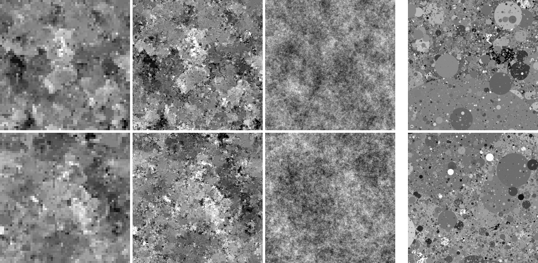
Figure 4: The model was trained on samples from an occlusion-based model [14]. Example images from the training set are given on the right. As above, the first two columns show samples from our model at two different scales. The third column shows the same samples with all higher-order correlations destroyed, revealing second-order statistics which are very similar to the ones learned from natural images.

As another test, we generated 1000 images of size $256\times 256$ pixels from an occlusion model (”dead leaves”) using the procedure described by Lee and Mumford in [14]. Afterwards, we added small Gaussian white noise. The model was designed to generate samples which share many properties with natural images. In particular, the samples are approximately scale-invariant and share very similar marginal and second-order statistics. Many of the difficult-to-capture higher-order correlations found in natural images are believed to be caused by occlusions in the image. This dataset should therefore pose similar challenges as the set of natural images. We extracted training data at three different scales and used the same training procedure as above. Clearly, our model has not learned what a circle is. However, it is able to reproduce the blotchiness of the original samples. This is especially surprising given the small size of the neighborhoods and the fact that the basic building block of our model is the Gaussian distribution. Also note that our model has no explicit knowledge of occlusions. As expected, destroying the higher-order correlations of the samples again leaves us with pink noise-like images (Figure 4).

3.1 Scale invariance and multi-information rates

The multiscale representation lends itself to an investigation of the scale invariance property of natural images. The statistics of a scale-invariant process are invariant under block-averaging and appropriate rescaling to compensate for the loss in variance [15]. Using the notation as above, this would mean that $X^{0}$ is distributed as $aX^{1}$ for some $a$. This in turn implies that the multi-information rate (MIR) should stay constant as a function of the scale. Because the MIR is invariant under rescaling with a constant factor, we can ignore the rescaling factor $a$.

Figure 5: Left: The estimated multi-information rate decreases steadily as the scale increases (the resolution decreases). Right: The conditional cross-entropy rate increases with scale. This shows that the van Hateren dataset [12] is generally not scale-invariant. A very similar behavior is shown by images created with an occlusion based model [14].

We estimated the multi-information rate of the van Hateren dataset with the cross-MIR of our model (Figure 5). The steady decrease of the information rate indicates that the statistics of images taken from the van Hateren dataset are not fully scale-invariant. A consequence of a smaller MIR is that pixels are more difficult to predict from neighboring pixels.

The difference in cross-MIR could also be caused by the fact that we are using a slightly different model at the largest scale than for modeling the image details at the lower scales. This problem is not shared by the conditional entropy rates plotted on the right of Figure 5. If scale invariance is given, the distribution over the high-resolution information $Y_{s}$ and the low-resolution information $X_{s}$ should not change with scale $s$, subject to proper rescaling. Since we are using the same model to model the relationship between $X_{s}$ and $Y_{s}$ for all $s$, the estimated entropy rates should stay constant even if our model performed poorly. Our results are consistent with the findings of Wu et al., who showed that many natural images are more difficult to compress at larger scales and argued that the entropy rate of natural images has to increase with scale [16].

Using an estimate of the marginal entropy of $1.57$ bits, we arrive at an estimated multi-information rate of $3.44$ bits per pixel for the van Hateren dataset (Figure 6). This is approximately $0.18$ bits better than the current best estimate for natural images [6] and $0.04$ bits better than our result obtained without using the multiscale representation.

Since the true MIR of natural images is unknown, this increase in performance does not tell us how much closer we got to capturing all correlations of natural images. It also does not reveal in which way the model has improved compared to other models. Samples and statistical tests can give us an indication. Figure 7 shows samples drawn from models suggested by Domke et al. [4] and Hosseini et al. [6], as well samples drawn using the extensions presented in this paper. The substantial change in the appearance of the samples suggests that even the increase from 3.40 bits to 3.44 bits is significant.

The joint statistics of the responses of two filters applied at different locations in an image are known to change in certain ways as a function of their spatial separation and are difficult to reproduce [17]. We apply a vertically oriented Gaussian derivative filter at two vertically offset locations and record their responses. After whitening, the filter responses are approximately $L_{p}$-spherically symmetric. We therefore fit an $L_{p}$-spherically symmetric model with a radial Gamma distribution to the responses and, at every distance, record the parameter $p$ of the model’s norm. Since the marginal distribution of each filter response is highly kurtotic and the responses become more independent as the filter distance increases, the joint histogram becomes more and more star shaped. This is expressed in the optimal value for $p$ becoming smaller and smaller. As plotted in Figure 6, the behavior of the optimal $p$ is not well reproduced using a single scale but is captured by our multiscale model.

multi-information rates

model	$I_{\infty}$ [bits]
MCGSM + multiscale	3.44
MCGSM	3.40
CGSM [6]	3.26
MCG [4]	3.25
CG (Gaussian)	2.70

Figure 6: Top right: Multi-information rate estimates of natural images obtained using different models. The multiscale representation allows us to obtain a somewhat better estimate. Bottom right: The joint histogram of pairs of Gaussian derivative filter responses changes as their spatial separation increases. Left: $L_{p}$-spherically symmetric distributions were fitted to the filter responses for natural and synthetic data. The vertical axis shows a maximum likelihood estimate of the parameter $p$. The horizontal axis shows the vertical offset between the position of the two filters. The plot shows that the multiscale representation enables our model to match the statistics of pairwise filter responses over much longer distances, which could be one possible explanation for the better performance.

Figure 7: From left to right: Samples from a mixture of conditional Gaussians [4] (5x5 neighborhoods, 5 components including means), a conditional Gaussian scale mixture [6] (7x7 neighborhoods, 7 scales), a mixture of conditional Gaussian scale mixtures and the multiscale model. The appearance of the samples changes drastically from model to model, indicating that the seemingly small improvements in bit/pixel are in fact substantial.

4 Conclusion

We have shown how to use directed models in combination with multiscale representations in a way which allows us to still evaluate the model in a principled manner. To our knowledge, this is the only multiscale model for which the likelihood can be evaluated. Despite the model’s computational tractability, it is able to learn interesting higher-order correlations from natural images and yields state-of-the-art performance when evaluated in terms of the multi-information rate. In contrast to the directed model applied to images at a single scale, the model also reproduces the pairwise statistics of filter responses over long distances. Here, we only used a simple multiscale representation. Using more sophisticated representations might lead to even better models.

References

- [1] J. L. Gallant and R. J. Prenger. Neural mechanisms of natural scene perception. The Senses: A Comprehensive Reference, 1:383–391, 2008.
- [2] J. A. Guerrero-Colon, E. P. Simoncelli, and J. Portilla. Image denoising using mixtures of gaussian scale mixtures. Proceedings of the 15th IEEE International Conference on Image Processing, 2008.
- [3] M.Bethge and R. Hosseini. Method and device for image compression. Patent WO/2009/146933, 2007.
- [4] J. Domke, A. Karapurkar, and Y. Aloimonos. Who killed the directed model? IEEE Computer Vision and Pattern Recognition, 2008.
- [5] M. Ranzato, V. Mnih, and G. E. Hinton. Generating more realistic images using gated mrf’s. Advances in Neural Information Processing Systems 23, 2010.
- [6] R. Hosseini, F. Sinz, and M. Bethge. Lower bounds on the redundancy of natural images. Vision Research, 2010.
- [7] M. Wainwright and E. P. Simoncelli. Scale mixtures of gaussians and the statistics of natural images. Advances in Neural Information Processing Systems 12, 2000.
- [8] Y. Weiss and W. T. Freeman. What makes a good model of natural images? IEEE Computer Vision and Pattern Recognition, 2007.
- [9] S. Lyu and E. P. Simoncelli. Statistical modeling of images with fields of gaussian scale mixtures. Advances in Neural Information Processing Systems 19, 2007.
- [10] R. A. Jacobs, M. I. Jordan, S. J. Nowlan, and G. E. Hinton. Adaptive mixtures of local experts. Neural Computation, 1991.
- [11] T. Cover and J. Thomas. Elements of Information Theory. Wiley, 2nd edition, 2006.
- [12] J. H. van Hateren and A. van der Schaaf. Independent component filters of natural images compared with simple cells in primary visual cortex. Proceedings of the Royal Society B: Biological Sciences, 1998.
- [13] J. Nocedal and S. J. Wright. Numerical Optimization, pages 136–143. Springer, 2nd edition, 2006.
- [14] A. B. Lee and D. Mumford. An occlusion model generating scale-invariant images. Proceedings of the IEEE Workshop on Statistical and Computational Theories of Vision, 1999.
- [15] A. B. Lee, D. Mumford, and J. Huang. Occlusion models for natural images: A statistical study of a scale-invariant dead leaves model. International Journal of Computer Vision, 2001.
- [16] Y. N. Wu, C.-E. Guo, and S.-C. Zhu. From information scaling of natural images to regimes of statistical models. Quarterly of Applied Mathematics, 2008.
- [17] F. Sinz, E. P. Simoncelli, and M. Bethge. Hierarchical modeling of local image features through -nested symmetric distributions. Advances in Neural Information Processing Systems 22, 2009.