Superconductor-insulator-ferromagnet-superconductor Josephson junction: From the dirty to the clean limit

Abstract

The proximity effect and the Josephson current in a superconductor-insulator-ferromagnet-superconductor (SIFS) junction are investigated within the framework of the quasiclassical Eilenberger equations. This investigation allows us to compare the dirty and the clean limits, to investigate an arbitrary impurity scattering, and to determine the applicability limits of the Usadel equations for such structures. The role of different types of the FS interface is analyzed. It is shown that the decay length $\xi_{1}$ and the spatial oscillation period $2\pi\xi_{2}$ of the Eilenberger function may exhibit a nonmonotonic dependence on the properties of the ferromagnetic layer such as exchange field or electron mean free path. The results of our calculations are applied to the interpretation of experimentally observed dependencies of the critical current density on the ferromagnet thickness in Josephson junctions containing a Ni layer with an arbitrary scattering.

I Introduction

Superconductor-ferromagnet-superconductor (SFS) Josephson junctions are a subject of intensive theoretical and experimental studies Golubov et al. (2004); Buzdin (2005); Bergeret et al. (2005). In particular, the question of the applicability range of predictions from dirty and clean limit theories and the treatment of the crossover between these two limits has been recognized as an important problem for the theoretical description of SFS structures Bergeret et al. (2001); Linder et al. (2009).

For the majority of experimental realizations of SFS structures Ryazanov et al. (2001); Oboznov et al. (2006); Blum et al. (2002); Sellier et al. (2003); Born et al. (2006); Weides et al. (2006a, b); Pfeiffer et al. (2008); Robinson et al. (2006, 2007) the exchange energy $H$ of the ferromagnetic materials is rather large Born et al. (2006); Robinson et al. (2006). As a consequence, the characteristic magnetic length $\xi_{H}=\hbar v_{f}/2H\lesssim\ell_{f}$, where $\ell_{f}$ is the electron mean free path and $v_{f}$ is the Fermi velocity in the F layer Ryazanov et al. (2001); Oboznov et al. (2006); Blum et al. (2002); Sellier et al. (2003); Born et al. (2006); Weides et al. (2006a, b); Pfeiffer et al. (2008); Robinson et al. (2006, 2007). Under this condition the numerous theoretical predictions Golubov et al. (2004); Buzdin (2005); Bergeret et al. (2005) based on the Usadel equations Usadel (1970) have a rather restricted range of validity; i.e. a more general approach based on the Eilenberger equations Eilenberger (1968) has to be developed.

A simple expression for the critical current density $J_{C},$ which is valid in the clean limit, was derived in Ref. Buzdin et al., 1982. Still the analysis of the Eilenberger equations for more general cases, remained a difficult problem. A significant progress along this direction has been achieved a decade ago Bergeret et al. (2001), where the solution of the Eilenberger equations for arbitrary scattering has been expressed in an integral form Bergeret et al. (2001). It was supposed Bergeret et al. (2001) that the SF interface transparency $D$ is small enough, providing the opportunity to use the linearized equations. Thus, a general expression for the Josephson junction supercurrent has been derived and used for numerical evaluations. The integral representation of the solution of the Eilenberger equations also permits to reproduce analytical expressions for $J_{C}$ obtained earlier within both clean and dirty limits Buzdin et al. (1982, 1992); Ryazanov et al. (2001). Recently, the same results have been achieved using the Ricatti parametrization of the one-dimensional Eilenberger equations Linder et al. (2009). However, the obtained expressions Bergeret et al. (2001) are so complicated that they are difficult analyze and use in practice. Although the use of a one-dimensional equation Linder et al. (2009) significantly simplifies the problem, it contains a non-controllable assumption about the insignificance of the angular distribution of the Eilenberger function.

Despite of this progress, it is still not clear within which range of parameters and with what accuracy it is possible to use simple expressions for the clean Buzdin et al. (1982) and dirty Buzdin et al. (1992) limits. The question about the influence of transport properties of SF interfaces is also still open. Since the answer to these questions is rather important for experimentalists, we formulate here a problem for a particular case of superconductor-insulator-ferromagnet-superconductor (SIFS) junctions. In comparison with SFS, in SIFS structures superconductivity is induced in the F layer only from one S electrode. This essentially simplifies the analysis compared to that for SFS junctions.

On the one hand, SIFS junctions are interesting by themselves as potential elements for superconducting logic circuits Terzioglu and Beasley (1998); Ioffe et al. (1999); Ustinov and Kaplunenko (2003) because it is possible to vary their critical current density in the $\pi$ state within a rather wide range, still keeping a high $J_{C}R_{N}$ product Weides et al. (2006b); Pepe et al. (2006), where $R_{N}$ is the junction normal resistance per square. Furthermore, in comparison with SFS junctions, SIFS junctions have very small damping which decreases exponentially at $T\to 0$. This makes them useful for superconducting circuits where low damping is required. On the other hand, an SIFS junction represents a convenient model system for a comparative study of 0-$\pi$ transitions for an arbitrary ratio of characteristic lengths in the F layer: the F-layer thickness $d_{f}$, the mean free path $\ell_{f}$, the characteristic magnetic length $\xi_{H}$, and the nonmagnetic coherence length $\xi_{0}=\hbar v_{f}/2\pi k_{B}T,$ where $T$ is the temperature.

To calculate $J_{C}$ of an SIFS junction, it is sufficient to study the proximity effect in the FS bilayer and to calculate the magnitude of the Eilenberger functions at the IF interface. For simplicity we will restrict ourselves to the study of the situation when the anomalous Green’s function induced in the F layer is small enough, permitting us to use the linearized Eilenberger equation for the description of the superconducting properties induced in the ferromagnet. Such an approximation is valid if the FS interface has a small transparency or if $T$ is close to the critical temperature $T_{c}$ of the S electrodes.

This article is organized as follows. In sec. II we describe our model based on the linearized Eilenberger equation supplemented with Zaitsev boundary conditions Zaitsev (1984) for an SIFS junction. Different types of FS boundaries are analyzed. Section III presents dependencies of anomalous Green’s functions and the critical current density on the F-layer parameters. The comparison with experimental results is presented in Section IV. Section V concludes this work. The calculation details can be found in the Appendix.

II Model

II.1 Proximity effect in the FS electrode

To analyze the proximity effect in an FS bilayer for arbitrary values of the electron mean free paths $\ell_{s}$ and $\ell_{f}$ in the S and F layer, respectively, it is convenient to introduce the following functions

$$\Phi_{+}=\frac{1}{2}\left[f(x,\theta_{s},\omega)+f^{+}(x,\theta_{s},\omega)\right],$$ (1)

$$\Phi_{-}=\frac{1}{2}\left[f(x,\theta_{s},\omega)-f^{+}(x,\theta_{s},\omega)\right],$$ (2)

where $f(x,\theta_{s},\omega)$ and $f^{+}(x,\theta_{s},\omega)$ are the quasiclassical Eilenberger functions Eilenberger (1968). Then we rewrite the Eilenberger equations for the S layer, located at $\ 0\leq x\leq\infty$, in the form:

$$\frac{k_{s}^{2}}{\ell_{s}^{2}\mu_{s}^{2}}\frac{\partial^{2}}{\partial x^{2}}\Phi_{+}-\Phi_{+}=-\frac{2\Delta\tau_{s}+\left\langle\Phi_{+}\right\rangle}{2\left|\omega\right|\tau_{s}+1},$$ (3)

where

$$\left\langle\Phi_{+}\right\rangle=\int_{0}^{1}\Phi_{+}d\mu,$$ (4)

$$\Phi_{-}=-\frac{\ell_{s}\operatorname{\mathrm{sign}}(\omega)}{k_{s}}\mu_{s}\frac{\partial}{\partial x}\Phi_{+}\;.$$ (5)

The insulating layer of negligible thickness is located at $x=-d_{f}$. In the F layer (located at $-d_{f}\leq x\leq 0$) the equations have the form

$$\frac{k_{f}^{2}}{\ell_{f}^{2}\mu_{f}^{2}}\frac{\partial^{2}}{\partial x^{2}}\Phi_{+}-\Phi_{+}=-\frac{\left\langle\Phi_{+}\right\rangle}{k_{f}},$$ (6)

$$\Phi_{-}=-\frac{\ell_{f}\operatorname{\mathrm{sign}}(\omega)}{k_{f}}\mu_{f}\frac{\partial}{\partial x}\Phi_{+}.$$ (7)

Here $\omega=\pi T(2n+1)$ are Matsubara frequencies, $\theta_{s,f}$ are the angles between the FS interface normal and the direction of Fermi velocities $v_{s,f}$ in the S and F layers, respectively, $\mu_{f,s}=\cos\theta_{f,s},$ $\Delta$ is the superconducting order parameter, which is assumed to be zero in the ferromagnet, $\tau_{s,f}=\ell_{s,f}/v_{s,f}$ are electron scattering times, and corresponding wave vectors $k_{s}=2\left|\omega\right|\tau_{s}+1,$ $k_{f}=2[\left|\omega\right|+iH\operatorname{\mathrm{sign}}(\omega)]\tau_{f}+1=2\left|\omega\right|\ell_{f}/v_{f}+i2H\ell_{f}/v_{f}\operatorname{\mathrm{sign}}(\omega)+1=1+\ell_{f}/\xi_{\omega}+i\operatorname{\mathrm{sign}}(\omega)\ell_{f}/\xi_{H},$ $\xi_{\omega}=v_{f}/2\left|\omega\right|.$ We use the units where $\hbar=1$ and $k_{B}=1$. Here we also take into account that the normal Eilenberger function in the ferromagnet $g\approx\operatorname{\mathrm{sign}}(\omega).$ We also neglect multiple reflections from the FS and the IF interfaces, which is reasonable if $d_{f}\geqslant\ell_{f}$, i.e. the ballistic regime is not considered. The fully ballistic case with a double barrier SIFIS junction was examined in Ref. [Radovic et al., 2003].

Equations (3)–(7) must be supplemented by the boundary conditions. At $x\rightarrow\infty$ the function $\Phi_{+}$ should approach its bulk value

$$\Phi_{+}(\theta_{s},\omega)=\frac{\Delta_{0}}{\sqrt{\Delta_{0}^{2}+\omega^{2}}},\$$ (8)

where $\Delta_{0}$ is the magnitude of superconductor order parameter far from the SF interface. At $x=-d_{f}$ the boundary condition

$$\frac{d}{dx}\Phi_{+}(-d_{f},\theta_{f},\omega)=0$$ (9)

guarantees the absence of a current across the insulating layer.

The boundary conditions at the FS interface strongly depend on its transport properties. Below we will assume for the FS interface transparency $D(\mu_{f})\ll 1$. Then to the first approximation we may neglect the suppression of superconductivity in the S electrode and rewrite the Zaitsev boundary conditions Zaitsev (1984) in the form

$$\frac{\ell_{f}}{k_{f}}\mu_{f}\frac{\partial}{\partial x}\Phi_{+}=D(\mu_{f})\frac{\Delta_{0}}{\sqrt{\Delta_{0}^{2}+\omega^{2}}}.$$ (10)

From the structure of Eilenberger equations (3)–(7) and the boundary conditions (8)–(10) it follows that

$$\Phi_{+}(\theta_{s},\omega)=\Phi_{+}(\theta_{s},-\omega),$$ (11a)

$$\Phi_{+}(\theta_{f},\omega)=\Phi_{+}^{\ast}(\theta_{f},-\omega),$$ (11b)

$$\Phi_{-}(\theta_{s},\omega)=-\Phi_{-}(\theta_{s},-\omega),$$ (12a)

$$\Phi_{-}(\theta_{f},\omega)=-\Phi_{-}(\theta_{f},-\omega).$$ (12b)

These symmetry relations permit us to consider the solution of the boundary problem formulated above only for $\omega>0.$

II.2 Solution of the Eilenberger equations in the F layer.

It is convenient to look for a solution of Eilenberger equations in the F layer (7) in the form

$$\Phi_{+}=\sum_{m=-\infty}^{\infty}Q_{m}\cos\left(\frac{\pi m(x+d_{f})}{d_{f}}\right)+B\cosh\left(\frac{x+d_{f}}{\ell_{f}\left|\mu_{f}\right|}k_{f}\right),$$ (13)

which automatically satisfies the boundary condition (9). The relation between the coefficients $Q_{m},$ and $B$ can be found by substitution of the ansatz (13) into the Eilenberger equation (6). Multiplying the obtained equations by $\cos[\pi k(x+d_{f})/d_{f}],$ and integrating them over $x$, one can easily find the relation between the coefficients $Q_{m},$ and $B$, see the Appendix. $B=B(\mu_{f})$ can be found from the boundary condition (10). Thus we arrive to the following expression for the Eilenberger function in the ferromagnet

$$\Phi_{+}=\frac{\Delta_{0}}{\sqrt{\Delta_{0}^{2}+\omega^{2}}}\left[\sum_{m=-\infty}^{\infty}\frac{\left\langle D(\mu)\frac{\mu}{q}\frac{\left(-1\right)^{m}}{M(\mu)}\right\rangle_{\mu}}{M(\mu_{f})\left[k_{f}-\left\langle\frac{1}{M}\right\rangle\right]}\cos\left(\frac{\pi m(x+d_{f})}{d_{f}}\right)+\frac{D(\mu_{f})}{\sinh\left(\frac{q}{\mu_{f}}\right)}\cosh\left(q\frac{x+d_{f}}{d_{f}\mu_{f}}\right)\right],$$ (14)

where

$$q=\frac{d_{f}k_{f}}{\ell_{f}}=d_{f}\left(\frac{1}{\ell_{f}}+\frac{1}{\xi_{\omega}}+i\frac{1}{\xi_{H}}\right).$$

Then the Eilenberger function averaged over the angle $\theta_{f}$ has the form

$$\left\langle\Phi_{+}\right\rangle=\frac{\Delta_{0}}{\sqrt{\Delta_{0}^{2}+\omega^{2}}}\sum_{m=-\infty}^{\infty}\frac{\left\langle D(\mu)\frac{\mu}{q}\frac{\left(-1\right)^{m}}{M(\mu)}\right\rangle_{\mu}}{\left[k_{f}-\frac{q}{\pi m}\arctan\left(\frac{\pi m}{q}\right)\right]}\cos\left(\frac{\pi m(x+d_{f})}{d_{f}}\right),$$ (15)

There are several interface models with a different $D(\mu_{f})$ dependence.

First, the FS interface may be represented by a thick diffusive barrier. Then the incident electron scatters in any arbitrary direction with equal probability, independent on the incident angle, i.e.,

$$D(\mu_{f})=D_{1}.$$ (16)

The second model considers an FS interface with a potential barrier, which appears due to different Fermi velocities in the S and F layer. The transmission coefficient in this case has the form

$$D(\mu_{f})=\frac{4v_{s}\mu_{s}v_{f}\mu_{f}}{\left(v_{s}\mu_{s}+v_{f}\mu_{f}\right)^{2}}\approx\frac{4v_{f}}{v_{s}}\mu_{f}=D_{2}\mu_{f},\quad\text{ if}\quad v_{s}\gg v_{f}\;.$$ (17)

It is necessary to note, that the incidence angle and the reflection angle are related by the expression

$$v_{s}\sin\theta_{s}=v_{f}\sin\theta_{f}.$$ (18)

Therefore, only the electrons which are at almost normal incidence to the interface ($\mu_{s}\approx 1$) may penetrate through the barrier. This model seems to be mostly reasonable for description of recent experiments Mattheiss (1970) with Nb electrodes ($v_{s}\sim 5\ldots 6\cdot 10^{7}\,\mathrm{cm/s}$) and 3$d$ ferromagnets or its Cu alloys Shelukhin et al. (2006) (for Ni $v_{f}\approx 2.8\cdot 10^{7}\,\mathrm{cm/s}$).

Third, one can model the FS interface as a high and narrow ($\delta$-function like) potential barrier between two metals with close Fermi-velocities. In this case

$$D(\mu_{f})=\frac{4v_{s}\mu_{s}v_{f}\mu_{f}}{\left(v_{s}\mu_{s}+v_{f}\mu_{f}+W\right)^{2}}\approx\frac{4v_{s}v_{f}}{W^{2}}\mu_{f}^{2}=D_{3}\mu_{f}^{2},\quad\text{if}\quad v_{s}\approx v_{f},$$ (19)

where $W$ is the strength of $\delta$-function like barrier.

For the above mentioned three models of the FS interface we have three possible expressions for $\Phi_{+}$ with different average values $\left\langle\Phi_{+}\right\rangle$, see (53)-(55) for details.

First, for $D(\mu_{f})=D_{1}$

$$\Phi_{+}=\frac{\Delta_{0}D_{1}}{\sqrt{\Delta_{0}^{2}+\omega^{2}}}\left[\sum_{m=-\infty}^{\infty}\frac{\frac{q}{2\pi^{2}m^{2}}\left(-1\right)^{m}\ln\left[\frac{\pi^{2}m^{2}}{q^{2}}+1\right]\cos\left(\frac{\pi m(x+d_{f})}{d_{f}}\right)}{\left(m^{2}\frac{\pi^{2}\mu_{f}^{2}}{q^{2}}+1\right)\left[k_{f}-\frac{q}{\pi m}\arctan\left(\frac{\pi m}{q}\right)\right]}+\frac{\cosh\left(q\frac{x+d_{f}}{d_{f}\mu_{f}}\right)}{\sinh\left(\frac{q}{\mu_{f}}\right)}\right].$$ (20)

Second, for $D(\mu_{f})=\mu_{f}D_{2}$

$$\Phi_{+}=\frac{\Delta_{0}D_{2}}{\sqrt{\Delta_{0}^{2}+\omega^{2}}}\left[\sum_{m=-\infty}^{\infty}\frac{\frac{q}{\pi^{2}m^{2}}\left(-1\right)^{m}\left(1-\frac{q}{\pi m}\arctan\frac{\pi m}{q}\right)\cos\left(\frac{\pi m(x+d_{f})}{d_{f}}\right)}{\left(m^{2}\frac{\pi^{2}\mu_{f}^{2}}{q^{2}}+1\right)\left[k_{f}-\frac{q}{\pi m}\arctan\left(\frac{\pi m}{q}\right)\right]}+\frac{\mu_{f}\cosh\left(q\frac{x+d_{f}}{d_{f}\mu_{f}}\right)}{\sinh\left(\frac{q}{\mu_{f}}\right)}\right].$$ (21)

Third, for $D(\mu_{f})=\mu_{f}^{2}D_{3}$

$$\Phi_{+}=\frac{\Delta_{0}D_{3}}{\sqrt{\Delta_{0}^{2}+\omega^{2}}}\left[\sum_{m=-\infty}^{\infty}\frac{\frac{q}{2\pi^{2}m^{2}}\left(-1\right)^{m}\left(1-\frac{q^{2}}{\pi^{2}m^{2}}\ln\left(\frac{\pi^{2}m^{2}}{q^{2}}+1\right)\right)\cos\left(\frac{\pi m(x+d_{f})}{d_{f}}\right)}{\left(m^{2}\frac{\pi^{2}\mu_{f}^{2}}{q^{2}}+1\right)\left[k_{f}-\frac{q}{\pi m}\arctan\left(\frac{\pi m}{q}\right)\right]}+\frac{\mu_{f}^{2}\cosh\left(q\frac{x+d_{f}}{d_{f}\mu_{f}}\right)}{\sinh\left(\frac{q}{\mu_{f}}\right)}\right].$$ (22)

These are the solutions of the linearized Eilenberger equation in the ferromagnet. The corresponding expressions for $\langle\Phi_{+}\rangle$ are given by Eqs. (57)-(59) in the Appendix.

Let us consider how these expressions reproduce the limiting cases of strong and weak scattering, for which the solutions are well-known Buzdin (2005); Golubov et al. (2004).

II.3 Dirty limit

If the electron mean free path is the smallest characteristic length i.e. $\ell_{f}\ll\xi_{H},\xi_{0},d_{f},$ the frequent nonmagnetic scattering permits averaging over the trajectories Usadel (1970). Then it is possible to write a closed system of equations for averaged functions. The linearization of the Usadel equations is allowed at the same conditions as for the Eilenberger equation.

The linearized Usadel equation in the ferromagnet has the form

$$\xi_{f}^{2}\frac{\partial^{2}}{\partial x^{2}}\left\langle\Phi_{+}\right\rangle+\frac{\left(\omega+iH\right)}{\pi T_{c}}\left\langle\Phi_{+}\right\rangle=0$$ (23)

where $\xi_{f}^{2}=D_{f}/2\pi T_{c},$ and $D_{f}=\ell_{f}v_{f}/3$ is the diffusion coefficient. The solution of Eq. (23) may be written as

$$\left\langle\Phi_{+}\right\rangle=A\cosh\left(\frac{x-d_{f}}{\xi_{f}}\sqrt{\frac{\omega+iH}{\pi T_{c}}}\right)$$ (24)

The boundary condition at $x=0$ reads Kupriyanov and Lukichev (1988)

$$\gamma_{B}\xi_{f}\frac{\partial}{\partial x}\left\langle\Phi_{+}\right\rangle=\frac{\Delta_{0}}{\sqrt{\Delta_{0}^{2}+\omega^{2}}}\;.$$ (25)

Substituting the expression (24) into the Usadel equation (23) one can find the coefficient

$$A=\frac{\Delta_{0}}{\gamma_{B}\sqrt{\Delta_{0}^{2}+\omega^{2}}}\frac{1}{\sqrt{\frac{\omega+iH}{\pi T_{c}}}}\frac{1}{\sinh\left(\frac{d_{f}}{\xi_{f}}\sqrt{\frac{\omega+iH}{\pi T_{c}}}\right)}.$$ (26)

Let us consider the previously obtained averaged Eilenberger function (15). For small $\ell_{f}$ the parameter $q$ is large and

$$1 + \ell_{f}/\xi_{\omega}+i\ell_{f}/\xi_{H}-\frac{q}{\pi m}\arctan\left(\frac{\pi m}{q}\right)\approx$$

$$\approx \frac{1}{3q^{2}}\left[\pi^{2}m^{2}+\frac{d_{f}^{2}}{\xi_{f}^{2}}\frac{\left(\omega+iH\right)}{\pi T_{c}}\right]$$

It is seen that the sums in (14) and (15) converge at $\pi^{2}m^{2}\approx 2\left(\omega+iH\right)d_{f}^{2}/d_{f}.$ At these values of $m$

$$\pi^{2}m^{2}\frac{\mu_{f}^{2}}{q^{2}}\approx\frac{2\left(\omega+iH\right)}{d_{f}}d_{f}^{2}\frac{\mu_{f}^{2}}{d_{f}^{2}}\ell_{f}^{2}\approx\frac{6\left(\omega+iH\right)}{v_{f}}\mu_{f}^{2}\ell_{f}\ll 1$$

and

$$\Phi_{+}\approx\frac{\Delta_{0}}{\sqrt{\Delta_{0}^{2}+\omega^{2}}}\left[\sqrt{\frac{\pi T_{c}}{\omega+iH}}\frac{\cosh\left(\sqrt{\frac{\pi T_{c}}{\omega+iH}}\frac{x+d_{f}}{\xi_{f}}\right)}{\gamma_{B}\sinh\left(\sqrt{\frac{\pi T_{c}}{\omega+iH}}\frac{d_{f}}{\xi_{f}}\right)}+\right.\left.\frac{D(\mu_{f})}{\sinh\left(\frac{q}{\mu_{f}}\right)}\cosh\left(q\frac{x+d_{f}}{d_{f}\mu_{f}}\right)\right],$$ (27)

where the suppression parameter $\gamma_{B}$ describes the electron transmission through the FS interface, see expressions (60)–(62). After averaging over $\theta_{f}$ the expression (27) coincides with (24) with $A$ given by (26). It turns out that in the dirty limit the first term of the expression (14) for the Eilenberger function plays the main role, as the second term reduces due to the spatial averaging (15), and the Eilenberger function $\Phi_{+}=\left\langle\Phi_{+}\right\rangle$.

II.4 Clean limit

For a larger electron mean free path $\ell_{f}$ the sum in (50) converges at

$$\pi^{2}m^{2}\frac{\mu_{f}^{2}}{q^{2}}\approx 1,\quad\frac{\pi m}{q}\approx\frac{1}{\mu_{f}}\;.$$

In the limit $\xi_{H}\ll\xi_{\omega}$ we have

$$k_{f}-\frac{q}{\pi m}\arctan\left(\frac{\pi m}{q}\right)\approx\ell_{f}/\xi_{\omega}+i\ell_{f}/\xi_{H}$$

and

$$\Phi_{+}=\frac{\Delta_{0}}{\sqrt{\Delta_{0}^{2}+\omega^{2}}}\left\{\left(\frac{\ell_{f}}{\xi_{\omega}}+\frac{i\ell_{f}}{\xi_{H}}\right)^{-1}\left\langle\frac{\mu D(\mu)}{\mu_{f}^{2}-\mu^{2}}\left[\frac{\mu_{f}\cosh\left(\frac{qm(x+d_{f})}{\mu_{f}d_{f}}\right)}{\sinh\frac{q}{\mu_{f}}}-\frac{\mu\cosh\left(\frac{qm(x+d_{f})}{\mu d_{f}}\right)}{\sinh\frac{q}{\mu}}\right]\right\rangle_{\mu}+\right.$$

$$+\left.\frac{D(\mu_{f})}{\sinh\left(\frac{q}{\mu_{f}}\right)}\cosh\left(q\frac{x+d_{f}}{d_{f}\mu_{f}}\right)\right\}.$$ (28)

In this limit, the first term in the square brackets in Eq. (14) is small in comparison with the second one. Thus, one may conclude that the first term in Eq. (14) plays the main role in the dirty limit, while the second term of Eq. (14) describes mainly the clean limit when trajectories of motion are essential.

II.5 Josephson current

To calculate the Josephson current $J$ of a SIFS ferromagnetic tunnel junction we start from the expression Golubov et al. (2004)

$$J = 4eN(0)v\pi T\sum_{\omega>0}\int_{-1}^{1}(\operatorname{\mathrm{Im}}g_{11})\cos\theta d(\cos\theta)=$$ (29)

$$= 4eN(0)v\pi T\sum_{\omega>0}\int_{0}^{1}(\operatorname{\mathrm{Im}}g_{11}^{a})\mu d\mu.$$

Here $N(0)$ is the density of state at the Fermi surface, $v$ is the Fermi velocity, $g_{11}$ is the matrix element of the antisymmetric part of the Eilenberger function that is define by the following expression:

$$\hat{g}^{a}=\frac{1}{2}\left[\begin{array}[]{cc}g(\theta)-g(-\theta)&f(\theta)-f(-\theta)\\ f^{+}(\theta)-f^{+}(-\theta)&-g(\theta)+g(-\theta)\end{array}\right].$$

We apply the tunnel hamiltonian approach and use the boundary conditions on the dielectric interface. These boundary conditions are matching the quasiclassical electron propagators $g$ and $f$ on both sides of the boundary. The boundary conditions may essentially depend on the quality of the interface. In the case of a nonmagnetic specularly reflecting boundary between two metals these conditions read Zaitsev (1984)

$$\hat{g}^{a}(R\hat{g}_{+}^{c2}+\hat{g}_{-}^{c2})=D_{I}\hat{g}_{-}^{c}\hat{g}_{+}^{c}.$$ (30)

$$\hat{g}_{1}^{a}=\hat{g}_{2}^{a}=\hat{g}^{a}.$$ (31)

Here $D_{I}$ and $R_{I}=1-D_{I}$ are the interface transparency and reflectivity coefficients, the index $1(2)$ labels the functions on the right (left) side from the boundary plane, and the symmetric parts of the quasiclassical Eilenberger functions are defined by the equalities

$$\hat{g}_{-}^{c}=\frac{1}{2}\left(\hat{g}_{1}^{c}-\hat{g}_{2}^{c}\right),\quad\hat{g}_{+}^{c}=\frac{1}{2}\left(\hat{g}_{1}^{c}+\hat{g}_{2}^{c}\right),$$ (32)

$$\hat{g}_{1,2}^{c}=\frac{1}{2}\left(\begin{array}[]{cc}g_{1,2}(\theta)+g_{1,2}(-\theta)&f_{1,2}(\theta)+f_{1,2}(-\theta)\\ f_{1,2}^{+}(\theta)+f_{1,2}^{+}(-\theta)&-g_{1,2}(\theta)-g_{1,2}(-\theta)\end{array}\right).$$

Assuming that the insulating layer transparency is small, $D_{I}\ll 1,R_{I}\approx 1$, and taking into account that $\hat{g}_{1}^{2}=\hat{g}_{1}^{2}=\hat{1}$, we can expand the boundary conditions (30) in powers of $D_{I}$.

For SIFS tunnel structures with $s$-wave pairing in the electrodes, in this limit it immediately follows that the functions $g_{2}(\theta)=g_{s}(\theta)$ and $f_{2}(\theta)=f_{s}(\theta)$ are independent on $\theta$ and coincide with the expressions for spatially homogeneous superconducting electrodes

$$f_{f} = F_{f}(\theta)\exp\left\{+i\varphi/2\right\},\quad f_{s}=F_{s}\exp\left\{-i\varphi/2\right\},$$

$$F_{s} = \frac{\Delta_{0}}{\sqrt{\omega^{2}+\Delta_{0}^{2}}},\quad\quad g_{s}=\frac{\omega}{\sqrt{\omega^{2}+\Delta_{0}^{2}}}\;.$$ (33)

Here $\Delta_{0}$ and $\varphi$ are the absolute value and the phase difference of the order parameter in the electrodes. The boundary conditions (30) reduce in this case to

$$\hat{g}^{a} = D_{I}\hat{g}_{-}^{c}\hat{g}_{+}^{c}=\frac{D_{I}}{4}(\hat{g}_{1}^{c}\hat{g}_{2}^{c}-\hat{g}_{2}^{c}\hat{g}_{1}^{c})=$$ (34)

$$= \frac{D_{I}}{4}\left(\begin{array}[]{cc}f_{1}f_{2}^{+}-f_{2}f_{1}^{+}&2(g_{1}f_{2}-f_{1}g_{2})\\ 2(f_{1}^{+}g_{2}-g_{1}f_{2}^{+})&f_{1}^{+}f_{2}-f_{2}^{+}f_{1}\end{array}\right).$$ (37)

Then the expression for the Josephson current (29) has the form

$$J = \frac{1}{2}eN(0)v\pi T\sum_{\omega=-\infty}^{\infty}\int_{-\pi/2}^{\pi/2}[f_{2}^{+}(\theta)f_{1}(\theta)-$$ (38)

$$- f_{2}(\theta)f_{1}^{+}(\theta)]\cos\theta\ d(\cos\theta).$$

Using the definition (1) and its symmetry properties (11) and (12), one can find the result for the Josephson current $J$ of the tunnel junction $J=J_{C}\sin\varphi$, where

$$J_{C}=\frac{8\pi T}{eR_{N}}\sum_{\omega>0}\Phi_{+}(\mu_{s})\int_{0}^{1}D_{I}(\mu_{f})\operatorname{\mathrm{Re}}\left[\Phi_{+}(\mu_{f})\right]\mu_{f}d\mu_{f}\;.$$ (39)

The Eilenberger function of the left electrode $\Phi_{+}(\mu_{s})$ is also defined by (8).

The thin insulating layer is considered as a high potential barrier for electrons. The transmission probability is inversely proportional to the exponent of a distance passed by an electron, i.e. $\sim\exp(-d_{I}/\cos\theta),$ where $d_{I}$ is the dielectric thickness. Namely, it can be found from the well known expression Landau and Lifshits (1961) for the transmission coefficient of a square potential barrier of a thickness $a$, that

$$D_{I}(a) = \frac{4k_{1}^{2}k_{2}^{2}}{4k_{1}^{2}k_{2}^{2}+(k_{1}^{2}+k_{2}^{2})^{2}\sinh^{2}(k_{2}a)}\approx$$ (40)

$$\approx \frac{4k_{1}^{2}k_{2}^{2}}{(k_{1}^{2}+k_{2}^{2})^{2}}\exp(-2k_{2}a),$$

if $k_{2}a\gg 1$. Here $k_{1}$ and $ik_{2}$ are wave vectors of particles outside and inside the barrier. The expressions for the transmission coefficient of the FS boundary (17),(19) were obtained in the same way. Taking into account that $a=d_{I}/\mu,$ one can write the dependence $D_{I}(\mu)$ in the form

$$D_{I}(\mu)=\widetilde{D_{0}}\exp\left(-\frac{\alpha}{\mu}\right).$$ (41)

Here $\alpha$ is a decaying coefficient, that depends on the thickness and material of the insulator. It is useful for a numerical calculation to redefine the value $\widetilde{D_{0}}=D_{0}\exp(-\alpha)$ , and finally

$$D_{I}(\mu)=D_{0}\exp\left(-\alpha\frac{1-\mu}{\mu}\right).$$ (42)

III Discussion

III.1 Main cases

First, we start from the analysis of the Eilenberger function $\Phi_{+}(x,\mu_{f})$, which describes the superconducting properties of a ferromagnetic Josephson junction. In the simplest case $\Phi_{+}(x,\mu_{f})$ is an exponential function $\Phi_{+}(x)\propto\exp(x/\xi),\ x\leqslant 0$, or a combination of exponential functions, with a complex coherence length Buzdin (2005); Golubov et al. (2004)

$$\xi^{-1}=\xi_{1}^{-1}+i\xi_{2}^{-1}.$$ (43)

Here $\xi_{1}$ describes the decay of the superconducting correlations at some distance from the FS boundary, while $\xi_{2}$ defines the period of LOFF oscillations Larkin and Ovchinnikov (1965); Fulde and Ferrell (1964). For the described FS structure, $\Phi_{+}(x,\mu_{f})$ is given by the expressions (14) and (20)-(22). Now we try to describe the main features of the proximity effect in an FS structure. If the superconducting layer is thick enough to be considered as semi-infinite, and if in-plane nonuniformities connected with sample preparation and the domain structure of the ferromagnetic film can be neglected, the structure has one geometric parameter — the ferromagnet thickness $d_{f}$. The properties of the F material give three more characteristic lengths: the electron mean free path in the ferromagnet $\ell_{f}$, the nonmagnetic coherence length $\xi_{0}$, and the characteristic magnetic length $\xi_{H}$. The main questions at this stage are: can the Eilenberger function be approximated by an exponential function, and what is the relation between $\xi_{1},\xi_{2}$ and the characteristic lengths mentioned above.

The Fermi velocity for usual ferromagnetic metals Shelukhin et al. (2006) is $v_{f}\sim 3\cdot 10^{7}\,\mathrm{cm/s}$, and if even the temperature $T\sim T_{c}$, $\xi_{0}\sim 100\,\mathrm{nm}$, i.e. $\xi_{0}$ is much larger than other parameters of the problem in usual cases. The value of $\xi_{0}$ is difficult to decrease. The gradual increase of $\ell_{f}$ leads to the following four cases:

1. $\ell_{f}\ll\xi_{H},d_{f}$ — the well investigated dirty limit. This condition allows averaging of the Eilenberger functions over trajectories and using the Usadel equations. $\Phi_{+}$ is given by the expression (24), and for a strong exchange field ($H\gg k_{B}T_{c}$), $\xi_{1}=\xi_{2}=\sqrt{2\ell_{f}\xi_{H}/3}$.

2. $\ell_{f}\sim\xi_{H},d_{f}$ — the intermediate case. The Usadel equations cannot be used, and one needs to solve the Eilenberger equations taking into account the $\Phi_{+}(\theta)$ dependence. Up to now the linearized equations were solved only for an SFS junction Bergeret et al. (2001); Linder et al. (2009), and the obtained expressions are so complicated that they are very difficult to analyze. This is the most interesting case for our analysis, which allows to find out when this case reduces to the dirty limit and under which conditions the Usadel equations are applicable.

3. $\xi_{H}\ll\ell_{f}<d_{f},\xi_{0}$ — the clean limit. Here, $\Phi_{+}(x,\theta)$ is defined mainly by the second term of Eq. (14), and Bergeret et al. (2001); Vedyayev et al. (2005) $\xi_{1}\sim\ell_{f}$, $\xi_{2}\approx\xi_{H}$.

4. $\ell_{f}\gg d_{f}$ — the ballistic regime cannot be considered within the framework of our approach, excluding the case $\xi_{1}\ll d_{f}$ when multiple reflections from the interfaces can also be neglected. The ballistic SFS junction was considered earlierBuzdin et al. (1982); Radović et al. (2001); Konschelle et al. (2008); Linder et al. (2009); Radovic et al. (2003); Zareyan et al. (2001), and the dependence $J_{C}(d_{f})$ cannot be presented as an exponent in the general case Radovic et al. (2003).

III.2 Analysis of cases 1-3

In all plots presented below we use the same normalization for all lengths: $x$, $d_{f}$, $l_{f}$, $\xi_{0}$, $\xi_{H}$, $\xi_{1}$, $\xi_{2}$. All of them are normalized to some unit length $\Xi$, which, in fact, can be chosen arbitrarily, e.g. $\Xi=1\,\mathrm{nm}$. Note that only the ratios between the lengths given above are important, i.e., if one divides the above list of lengths by any arbitrary constant $\Xi$ all the results remain unchanged. For example, in all plots we use $\xi_{0}=81$.

Influence of different types of FS boundary transparency.

Figure 1 shows the spatial distribution of the functions $\langle\Phi_{+}(x)\rangle$ calculated from (4) for $\ell_{f}=7,\ \xi_{H}=3$, $d_{f}=10$ and $J_{C}(d_{f})$ calculated from (39) for $\ell_{f}=7,\ \xi_{H}=3$, and the insulating layer decay parameter $\alpha=5$. It is clearly seen that the angular dependence of SF interface transparency influences both, the amplitude and period of oscillations of the presented curves. For the particular choice of parameters this influence can be easily explained.

For the case of a transparency which is independent on $\mu_{f}$, the Eilenberger functions are initiated from the SF interface in all directions, thus leading to the largest amplitude of $\langle\Phi_{+}(x)\rangle$ oscillations. Simultaneously, the contributions to $\langle\Phi_{+}(x)\rangle$ coming from rapidly decaying Eilenberger functions with a large argument $\theta_{f}$ result in the appearance of the smallest period of $\langle\Phi_{+}(x)\rangle$ oscillations. The stronger the angular dependence of the SF interface transparency coefficient, the smaller are the contributions to average values from the rapidly decaying Eilenberger functions, and as the result the larger is the period and the smaller is the amplitude of $\langle\Phi_{+}(x)\rangle$ oscillations. It is necessary also to mention that $\langle\Phi_{+}(x)\rangle$ decays more rapidly with $|x|$ than $\Phi_{+}(x,1)$. This difference is the smaller the smaller is $l_{f}.$

From (39) it follows that in general the contribution to the junction critical current comes not only from $\Phi_{+}(x,1)$, but also from $\Phi_{+}(x,\mu_{f})$ located in a narrow domain of $\mu_{f}$ nearby $\mu_{f}=1.$ Due to that, the $J_{C}(d_{f})$ curve appears to be sensitive against the angular dependence of the SF interface transparency. We see that the stronger this dependence the smaller is the amplitude of oscillations and the larger are the distances of the $0$ to $\pi$ transition points in $J_{C}(d_{f})$ from the SF interface, while the period of $J_{C}(d_{f})$ oscillations is practically insensitive against the form of $D(\mu_{f})$ and coincides with that of $\Phi_{+}(x,1).$ If the ferromagnetic layer is thick enough, the sum over $\omega$ in (39) converges rapidly, and the main contribution is given by the first term of the sum, which is determined by the real part of the Eilenberger function $\Phi_{+}(x,1)$. For these reasons we will focus below on the examination of the properties of the real part of the Eilenberger function $\Phi_{+}(x,1)$, and in further calculations we will also use the form $D(\mu_{f})=D_{2}\mu_{f}$ for the transmission coefficient of the FS interface, as it is most applicable to materials used in experiments.

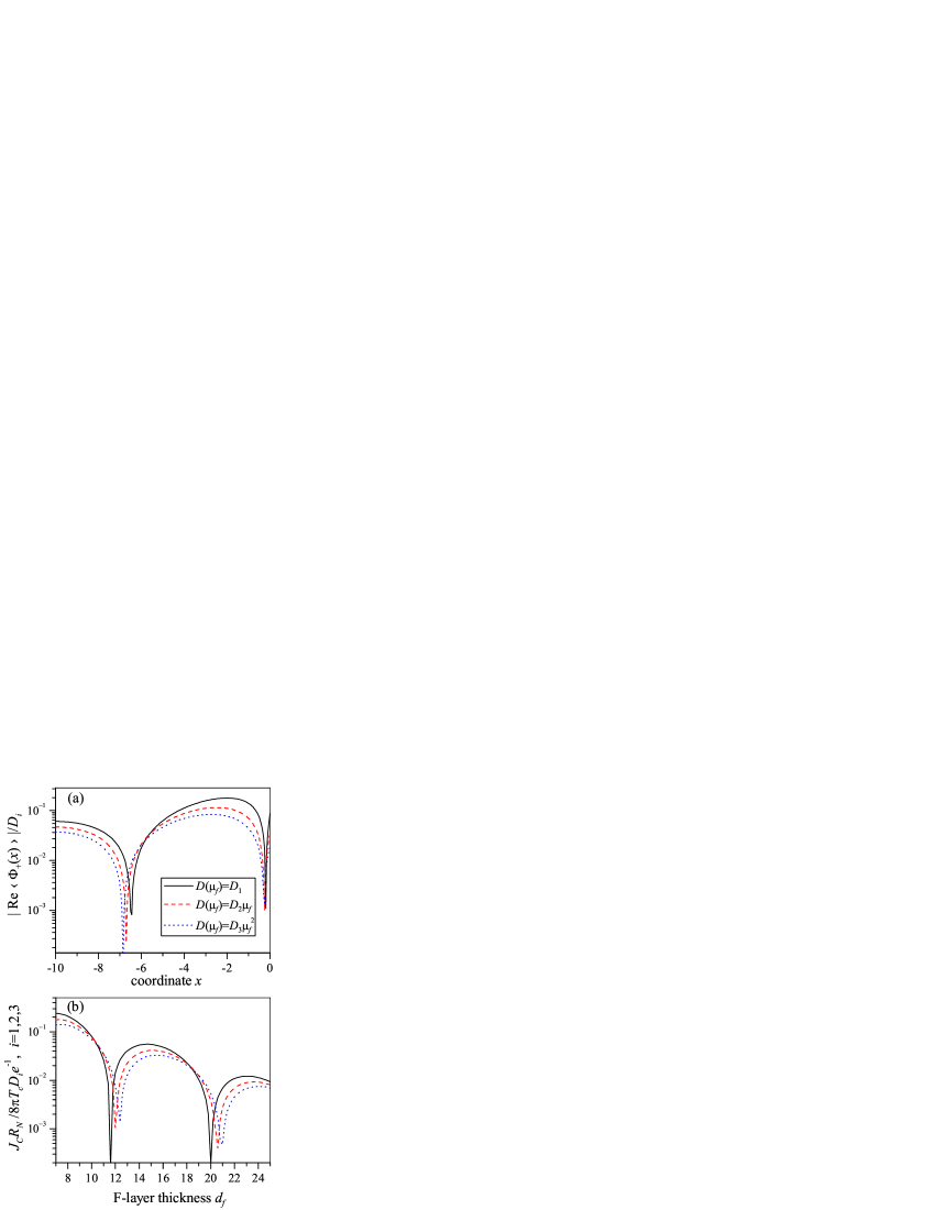
Figure 1: (Color online) (a) Averaged Eilenberger function $\langle\Phi_{+}(x)\rangle$ and (b) $J_{C}(d_{f})R_{N}$ product for different types of the FS interface (16)-(19). The F-layer parameters are $\ell_{f}=7,\ \xi_{H}=3$ (a,b), $d_{f}=10$ (a), the insulating layer decay parameter is $\alpha=5$ (b); $T\approx 0.5T_{c}$.

Spatial profile of the Eilenberger function.

The direct comparison (see Fig. 2) of the results of numerical calculations of the real part of the Eilenberger function $\Phi_{+}(x,1)$, making use of Eq. (21), with the curves which follow from the simple analytical expression

$$\Phi_{+}^{app}(x,1)\approx\frac{\Phi_{+}(0,1)}{\cosh(d_{f}/\xi)}\cosh\frac{x+d_{f}}{\xi}$$ (44)

confirms that it is possible to approximate $\Phi_{+}(x,1)$ by this simple formula. It satisfies the boundary condition on the dielectric interface (9) and contains the factor $\Phi_{+}(0,1)$, which has been calculated numerically from (21).

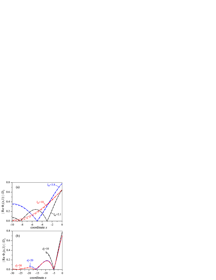
Figure 2: (Color online) The exact $\Phi_{+}(x,1)$ (solid lines) and approximated $\Phi_{+}(x,1)^{app}$ (dashed lines) Eilenberger function (a) for different values of $\xi_{H}$ corresponding to a local maximum, minimum, and smooth region of the dependence $\xi_{1}(\xi_{H})$; see Fig.3(b), at $\ell_{f}=7,\ d_{f}=10$; (b) for different thicknesses $d_{f}$ at $\ell_{f}=7,\ \xi_{H}=3.8$. $T\approx 0.5T_{c}$.

The quality of the approximation (44) was checked for different values of parameters for all dependencies investigated further. It was found to be satisfactory in the whole accessible range of parameters $d_{f}>\ell_{f}\ \mathrm{\ or}\ \xi_{1}$. This approximation yields the values of $\xi$, i.e. $\xi_{1}\ \mathrm{\ and}\ \xi_{2}$.

Dependence of $\xi$ on the junction parameters.

The attempt to find $\xi$ in the area of intermediate scattering was made earlier Yu.Gusakova et al. (2006). It was supposed in Ref. [Yu.Gusakova et al., 2006] that $\xi$ may be found as a solution of the equation

$$i\ell_{f}/\xi=\arctan(i\ell_{f}/k_{f}\xi),$$ (45)

which determines the poles of the sum in Eqs.(14), (15) for $\Phi_{+}(x)$ and $\langle\Phi_{+}(x)\rangle,$ respectively. Unfortunately, the inverse tangent is a multivalent function. In the general case this fact prevents to represent $\Phi_{+}(x)$ and $\langle\Phi_{+}(x)\rangle$ as only the sum of residues of summable functions in (14), (15). An exception occurs in the range of parameters for which the ferromagnet is close to the dirty limit. In this case the sum in (14) and (15) converts faster than the multivalent nature of the inverse tangent becomes essential. These difficulties had been first pointed out in Ref. [Volkov et al., 2006], where it was also demonstrated that the solution of the Eilenberger equations used in Ref. [Yu.Gusakova et al., 2006] does not transfer correctly to the solution of the Eilenberger equations in the clean limit.

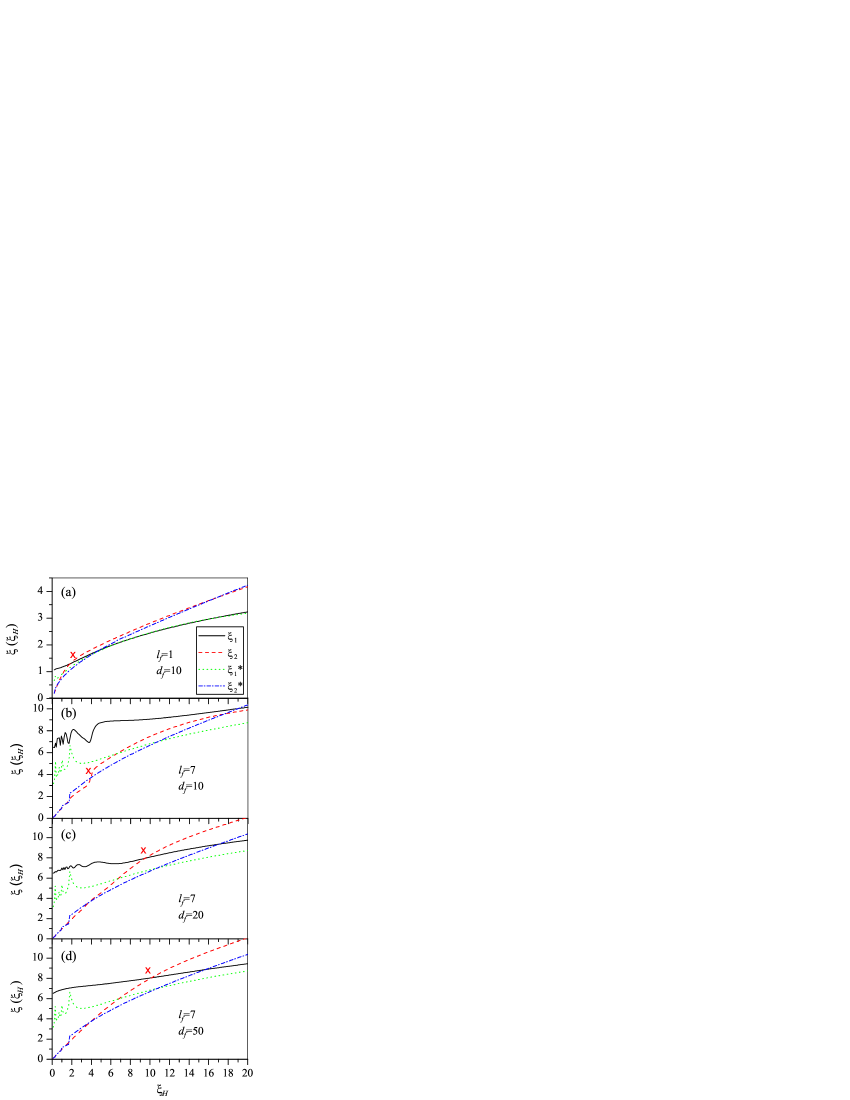
Figure 3: (Color online) Decay length $\xi_{1}$ and oscillation parameter $\xi_{2}$ vs magnetic length $\xi_{H}$ for different values of $\ell_{f}$ and $d_{f}$, that are denoted in the plots. The corresponding values of $\xi$ from Ref. [Yu.Gusakova et al., 2006] are also shown and marked by $*$.

To avoid these mathematical difficulties we have decided to find out the dependence $\xi(\xi_{H},\ell_{f})$ from the direct fitting of the real part of $\Phi_{+}(x)$ calculated numerically from (14) by approximating formula (44). The result of this procedure is demonstrated in Fig. 3. It shows the dependencies of $\xi_{1}\mathrm{\ and}\ \xi_{2}$ on the magnetic length $\xi_{H}$ at different $\ell_{f}$. The solutions from Ref. [Yu.Gusakova et al., 2006] are also presented in Fig. 3 for comparison. They coincide with our values when $\xi_{H}\gg\ell_{f}$ i.e. in the dirty limit. We have taken two cases for the numerical investigation: $\ell_{f}=1$, that is close to the dirty limit, and $\ell_{f}=7$, that is close to the clean case.

It is seen, that $\xi_{1}$ oscillates with the exchange energy $H$ (so as $\xi_{H}\sim H^{-1}$), an interesting result, that was not noted earlier. These oscillations appear in rather clean samples $\ell_{f}\gtrsim d_{f}/\pi$ and for $\xi_{H}<d_{f}/\pi$. They originate mainly from the second term of the expression (14), which plays the main role in the clean case. The function $\xi(\xi_{H})$ changes with increasing $d_{f}$ (cf. Fig. 3(b–d)). At large enough $d_{f}$, electrons have a time to scatter in the ferromagnet, their trajectories shuffle, and the dominant role of the ”clean“ term vanishes, the oscillations disappear, see Fig. 3(d). We note that the smaller is the probability of dephasing of the Eilenberger functions due to electron scattering in the F layer, the stronger are the interference effects between the IF and FS interfaces. This interference demands, for given values of $\xi_{1}$ and $\xi_{2}$, the fulfillment of the boundary conditions at these interfaces, which fix the value of the phase derivatives at $x=0$ and $x=d_{f}$. As it follows from Eq. (20)-(22), these conditions cannot be satisfied on the class of monotonic $\xi_{1}$ and $\xi_{2}$ functions. Therefore the transition from the dirty to the clean limit should be accompanied by a nonmonotonic behavior of $\xi_{1}$ and $\xi_{2}$ as a function of $\xi_{H}$ for fixed $\ell$, see Fig. 3, or as a function of $\ell$ for fixed $\xi_{H}$, see Fig. 4.

In the dirty limit the spatial oscillation length $\xi_{2}\approx\sqrt{2\ell_{f}\xi_{H}/3}$, while in the clean limit $\xi_{2}\approx\xi_{H}$. Near the point marked by X in Fig. 3 there is a crossover between the dependencies corresponding to dirty and clean limits, respectively, i.e. this region can be considered as a boundary between the clean and the dirty cases.

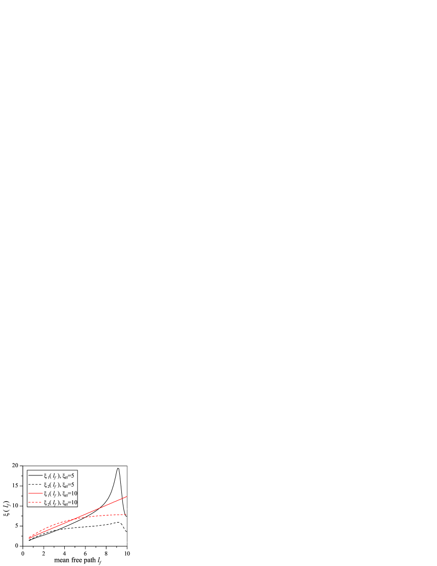
Figure 4: (Color online) Decay length $\xi_{1}$ (solid lines) and oscillation parameter $\xi_{2}$ (dashed lines) vs electron mean free path $\ell_{f}$ in the ferromagnet for different values of $\xi_{H}$; here $d_{f}=10$, $T\approx 0.5T_{c}$.

The dependence of $\xi$ on the mean free path $\ell$ for different $\xi_{H}$ is presented in Fig. 4. Usually the decay length $\xi_{1}$ as well as the oscillation period $2\pi\xi_{2}$ increase with the mean free path, which corresponds to the results in Ref. [Linder et al., 2009]. However, the dependence $\xi(\ell_{f})$ may be nonmonotonic for some values of the ferromagnet thickness.

In the presented figures one can see, that $\xi_{1}$ may be larger or smaller than $\xi_{2}$ and may behave nonmonotonically. This depends not only on the material constants of ferromagnetic material, but also on the thickness of the F layer.

The found values $\xi_{1}\ \mathrm{\ and}\ \xi_{2}$ together with the simple dependence (44) could be widely used for various estimations, approximate calculations, and fitting experimental data, for example for a measurement of the density of states (DOS) in an FS bilayer or calculation of thickness dependence of the critical current of SIFS Josephson junctions.

$J_{C}(d_{f})$ in the limit of large $d_{f}$.

As an example, we consider the critical current of SIFS Josephson junctions in the limit of large F layer thickness $d_{f}\gg\xi_{1}$. In this limit the main contribution to the critical current in (39) is given by the term at $\omega=\pi T.$ Suppose further that only electrons, that are incident in the direction perpendicular to the FI interface, provide the current across it, from (39), (44) we have

$$J_{C}=\frac{8\pi TD_{2}}{eR_{N}}\operatorname{\mathrm{Re}}{\frac{\Delta_{0}\Phi_{+}(0,1)}{\sqrt{(\pi T)^{2}+\Delta_{0}^{2}}\cosh(d_{f}/\xi)}}$$ (46)

The comparison with the exact numerical calculation has shown that this expression (46) well approximates $J_{C}(d_{f})$ starting from $d_{f}\gtrsim\xi_{1}$. The thickness dependence of $J_{C}$ calculated from (46) at the value $\xi$ taken at $d_{f}=50$, see Fig.3(d), for $l_{f}=7$, $\xi_{H}=2.1$, $T\approx 0.5T_{c}$ is shown in Fig. 5 by the solid line. The dashed and dashed dotted curves in Fig. 5 give the results obtained by numerical calculation, which have been done for the same parameters with the use of the exact expression for $\Phi_{+}(-d_{f},\mu_{f})$ in (39) and at different insulating layer thicknesses described by the parameter $\alpha.$

It is clearly seen that the larger is $\alpha$ the closer is the the result to the approximation formula (46). We may also conclude that the difference between the asymptotic solid curve and the dashed curves in Fig. 5 calculated for finite values of $\alpha$ occurs only in amplitude and positions of the $0$ to $\pi$ transition points, while the decay length and period of $J_{C}(d_{f})$ oscillations are nearly the same. This means, that if in experiment we are mainly interested in the estimation of the ferromagnet material constant, $\xi,$ we may really use for the data interpretation the simple expression (46) and consider the coefficient $\Phi_{+}(0,1)$ in it as a phenomenological parameter, which depends not only on the properties of ferromagnetic material, but also on $d_{f}$ in a rather complicated way, see Fig.2(b), as well as on the form of the transparency coefficients at the FI and FS interfaces. Although our results for SIFS junctions give the same $\xi_{1}$ and $\xi_{2}$ as for SFS junctions (at least for a thick F layer), different boundary conditions result in different order parameter amplitude and phase. This results in a different $J_{C}(d_{f})$ dependence, similar to the results obtained earlier in dirty limit Vasenko et al. (2008).

It is interesting to note that in the case of a rather thin insulating barrier and rather clean ferromagnet, $\xi_{1}\ \mathrm{\ and}\ \xi_{2}$ as measured from the critical current of SIFS junctions may differ from $\xi$ as measured from the DOS on the free F surface of an analogous FS bilayer. This is because the DOS measured by low-temperature scanning tunneling spectroscopy (which may only yield contributions from electrons with normal incidence) is directly given by $\Phi_{+}(-d_{f},\mu_{f}=1)$, while $J_{C}$ includes contributions from other angles.

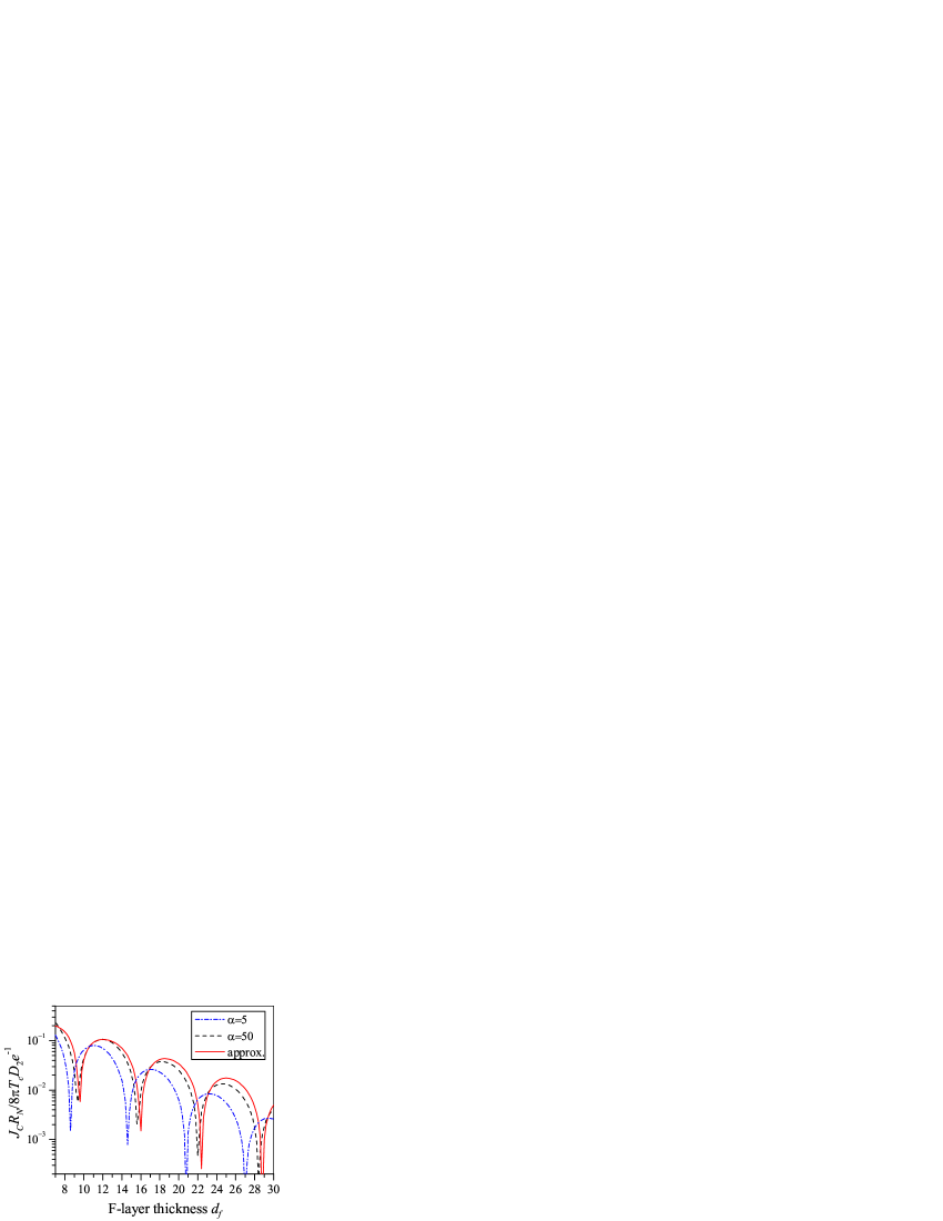
Figure 5: (Color online) $J_{C}R_{N}$ product as a function of the ferromagnet thickness $d_{f}$ at different insulating layer thicknesses described by the parameter $\alpha$, and the approximation by expressions (39),(44) at the value $\xi$ taken at $d_{f}=50$, see Fig.3(d), here $l_{f}=7$, $\xi_{H}=2.1$, $T\approx 0.5T_{c}$,.

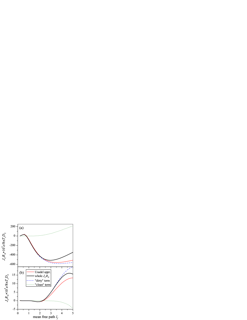
Figure 6: (Color online) $J_{C}R_{N}$ product vs ferromagnet mean free path $l_{f}$ ($\xi_{H}=10$, $T\approx 0.5T_{c}$, $\alpha=5$) for $d_{f}=10$ (a) and $d_{f}=30$ (b). Each plot shows $J_{C}R_{N}$ obtained from the Usadel function (15), from the Eilenberger function $\Phi_{+}$ (21), as well as from only the first ”dirty” term or only the second ”clean” term of (21).

Applicability of the Usadel equation.

The condition that allows using the Usadel equation is well known — this is strong nonmagnetic scattering Usadel (1970), namely, $\ell_{f}\ll\xi_{H},d_{f},\xi_{0}$. What does the symbol ”$\ll$“ mean exactly? In order to illustrate this, Fig. 6 shows the dependence $J_{C}(\ell_{f})$ given by the expression (21). Two parts of (21), called for convenience ”dirty” and ”clean”, are given by the first and the second terms of the expression (21). The critical current density as given by the Usadel function (27), describing the dirty limit, is also shown. $J_{C}(\ell_{f})$ coincides with the Usadel solution at $\ell_{f}\approx 0.1\xi_{H}$, then the first term in square brackets in Eq. (21) dominates and the $\mu_{f}$-dependence becomes nonsignificant due to the spatial averaging as a result of multiple scattering. This means, that the Usadel equations become appropriate to use if the parameter $H\tau_{f}\leqslant 0.1$. This result was intuitively clear, but demanded a proof due to plenty of investigations, where the Usadel equations was used at $H\tau_{f}\lesssim 1$.

IV Comparison with experiment

There are only few experiments on SIFS tunnel junctions with moderate scattering in the F-layer Born et al. (2006); Bannykh et al. (2009). In Ref. [Born et al., 2006] experimental data points for $J_{C}(d_{f})$ are rather sparse, while in Ref. [Bannykh et al., 2009] the density of data points per period is much larger. We thus decided to compare our theory to the data of Ref. [Bannykh et al., 2009].

This article Bannykh et al. (2009) also contains attempts to fit the experimental data by theoretical curves, however, without much success. Some of these attempts, see Fig.5(a) in Ref. [Bannykh et al., 2009], use a theory developed for a very clean (ballistic) SFS junction. The predicted oscillation period of $J_{C}(d_{f})$ was significantly smaller than the one in the experiment. Figure 5(b) in Ref. [Bannykh et al., 2009] shows the same experimental data together with fits using dirty limit theory. The best fit was achieved with $\xi_{1}=0.66\,\mathrm{nm}$ and $\xi_{2}=0.53\,\mathrm{nm}$. However, the theory for a dirty ferromagnetic junction cannot explain $\xi_{1}>\xi_{2}$, and all of these theories, both clean and dirty, do not take into account the insulating layer.

In Ref. [Bannykh et al., 2009] and Ref. [Weides, 2008] it was found, that the magnetic anisotropy of the F layer changes from perpendicular to in-plane with an increase of the F-layer thickness. Perpendicular magnetic anisotropy in a polycrystalline thin film may occur due to several reasons: the mechanism described by Neel Neel (1953) related to the absence of nearest neighbor F-layer atoms near interfaces, the magneto-striction mechanism, the surface roughness, and the one associated with microscopic-shape anisotropy Maissel and Glang (1970). The latter may also vary for samples sputtered under different angles Maissel and Glang (1970). Perpendicular magnetic anisotropy can change to an in-plane anisotropy due to a competition with the shape anisotropy of a film. However, none of the mechanisms listed above can be expected to give a significant jump of the exchange magnetic energy $H$ at the transition between the two types of anisotropy. There is some shift of the experimental curve, see Fig.2(a) in Ref. [Bannykh et al., 2009], at $d_{f}=3.8\,\mathrm{nm}$, where the anisotropy changes. But there are no reasons to assume, that this change of anisotropy is associated with a significant change of $H$. Therefore, we try to describe the whole experimental curve $J_{C}(d_{f})$ using the same value of $H$.

The common problem for all explanations of this experiment is the location of the first minimum of $J_{C}(d_{f})$ at a rather large $d_{f}\approx 3\,\mathrm{nm}$ in comparison with the oscillation length $\xi_{2}\approx 0.5\,\mathrm{nm}$. The authors Bannykh et al. (2009) attribute this to the existence of a nonmagnetic dead layer with rather large thickness $d_{dead}=2.26\,\mathrm{nm}$ in the Ni layer.

We note, that $d_{dead}$, in general, depends on $d_{f}$. We assume that $d_{dead}=d_{f}$ up to some value $d_{max}$ and then either $d_{dead}$ stays constant at a saturation value $d_{dead}^{sat}=d_{max}$ with further increase of $d_{f}$, or it is reduced to a constant value $d_{dead}^{sat}<d_{max}$. For the latter case there are the following reasons. The dead layer may consist of a nonmagnetic Ni alloy with magnetic clusters or islands, which are not connected by the exchange interaction. A very thin film of a ferromagnetic material may be paramagnetic. When one covers it by extra magnetic layers, some part of its thickness may magnetize. First, magnetic clusters uncoupled by the exchange interaction can couple if they are covered by extra magnetic layers. Second, a thin homogeneous film of a magnetic material of the thickness of a few monolayers exhibits nonmagnetic properties alone, but becomes magnetic entirely when its thickness increases, due to the transition from the two-dimensional to the three-dimensional case.

The dead layer is described as a normal layer, that yields $J_{C}(d_{f})\sim\exp(-\frac{d_{f}}{\xi_{N}})$. The best fitting presented in Fig. 7(a),(b) by straight short-dashed lines, gives the valueBannykh et al. (2009) $\xi_{N}=0.68\,\mathrm{nm}$. The normal metal coherence length $\xi_{N}$ depends both on the nonmagnetic and paramagnetic scattering. The latter may be significant in the dead layer in the presence of many magnetic inhomogeneities (clusters and impurities). Following a theory developed for SFS junctionsOboznov et al. (2006) taking into account magnetic scattering, one can find the expression for the coherence length of a normal metal (at $H=0$) with magnetic impurities $\xi_{N}=\sqrt{\frac{D_{f}}{2\left(\pi T+1/\tau_{m}\right)}}$, where $\tau_{m}$ is the magnetic scattering time. We assume that the mean free path has the same value as in the rest of the magnetic Ni layer, $\ell_{f}=0.6\,\mathrm{nm}$, that is given by the fit. This yields $\tau_{m}=1.68\cdot 10^{-14}\,\mathrm{s}$. For comparison, the nonmagnetic scattering time is found to be almost 8 times less. Fig. 7(a),(b) shows that the obtained value of $\xi_{N}$ is very close to the decay length of the magnetic SIFS junction at $d_{f}>d_{max}$. In the absence of the exchange field its pair-breaking role is played by the magnetic scattering in this structure.

We consider two possibilities to explain the experimental data Bannykh et al. (2009). First, we assume that the detected minimum of $J_{C}(d_{f})$ is the first one, see Fig. 7(a). Treating the dead layer as a normal layer ($H=0$), our best fit yields $d_{dead}^{sat}=d_{max}=2.37\,\mathrm{nm}$. The fitting yields the following values of the F-layer parameters: $\ell_{f}=0.6\,\mathrm{nm}$ and $\xi_{H}=0.6\,\mathrm{nm}$, that corresponds to $H=1782\,\mathrm{K}$ or $H=154\,\mathrm{meV}$.

As a second scenario we assume that the detected minimum of $J_{C}(d_{f})$ is the second one, see Fig. 7(b). The first $J_{C}(d_{f})$ minimum may not show up if the effective thickness of the dead layer decreases as soon as $d_{f}$ is above the threshold value $d_{max}$. Then, at the value of $d_{f}$ where $J_{C}(d_{f})$ is supposed to have the first minimum, the F layer may still be nonmagnetic, while at large values of $d_{f}$ it has some small value $d_{dead}^{sat}$. For that scenario $d_{dead}^{sat}=0.2\,\mathrm{nm}$ provides the best fit. The mean free path was found as $\ell_{f}=0.6\,\mathrm{nm}$, $\xi_{H}=0.956\,\mathrm{nm}$, that corresponds to $H=1119\,\mathrm{K}$ or $H=96.4\,\mathrm{meV}$.

In both fits we used the following parameters. The temperature $T=4.2\,\mathrm{K}$ and $T_{c}=8\,\mathrm{K}$ were taken like in the experimentBannykh et al. (2009), that yields $\xi_{0}=81\,\mathrm{nm}$. Fermi velocities Shelukhin et al. (2006) $v_{f}=2.8\cdot 10^{7}\,\mathrm{cm/s}$ and Mattheiss (1970) $v_{s}=6.2\cdot 10^{7}\,\mathrm{cm/s}$ were taken. Since $v_{s}>v_{f}$, we use the FS boundary condition in the form (17). The thickness of the insulating $\mathrm{Al_{2}O_{3}}$ barrier was not measured exactly; still the value $\alpha=5$ seems to be realistic, see Eq.(42). The values of the exchange field for both cases are within the range obtained for Ni in SFS experimentsRobinson et al. (2007, 2006); Blum et al. (2002); Shelukhin et al. (2006). The relation $\ell_{f}\sim\xi_{H}$ does not allow using the Usadel equations, however, this is not far from the dirty limit.

Comparing both fits shown in Fig. 7(a),(b) we cannot give a definite answer which minimum (the first or the second) was observed in the experiment Bannykh et al. (2009), but we are able to explain the fact that $\xi_{1}>\xi_{2}$ in any case. Such relation between $\xi_{1}$ and $\xi_{2}$ cannot be obtained from a dirty limit theory.

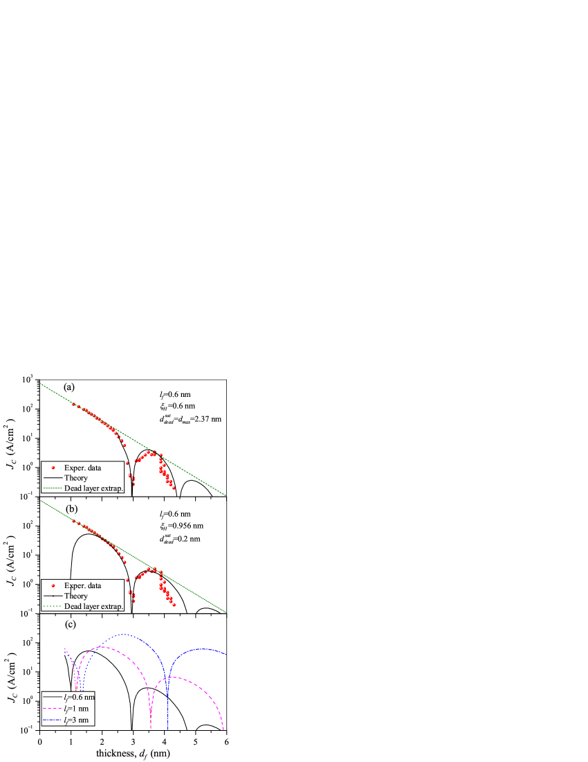
Figure 7: (Color online) (a) and (b) show a comparison of $J_{C}(d_{f})$ from the presented theory with experiment Bannykh et al. (2009). Dashed lines are fits to the experimental data in the range $d_{f}<2.37\,\mathrm{nm}$, where the F layer can be interpreted as nonmagnetic. (c) Dependencies $J_{C}(d_{f})$ at lower scattering. Parameters are like in (b). The regime for which multiple reflections cannot be neglected are marked by dotted lines.

The Josephson junctions used in the experiment Bannykh et al. (2009) contain an extra normal layer of Cu between the I and F layer. A normal layer cannot change $\xi$, which mainly depends on properties of the magnetic layer. However, it may change the boundary conditions. Therefore, our theory cannot be directly applied for the determination of the exact value of the dead layer, but may explain the obtained value of $\xi$.

For the analysis of the first minimum position and the dead layer estimation we may also use the theory developed earlier for the dirty limit, since the estimated value of $\ell_{f}\sim\xi_{2}$. From the analysis of the uniform part of the solutions obtained in Ref. [Pugach et al., 2009] for dirty SINFS and SIFNS junctions, it follows that the first minimum of the $J_{C}(d_{f})$ dependence must be at $(d_{f}-d_{dead})/\xi_{2}\approx 3\pi/4$. If we assume that the detected minimum of $J_{C}(d_{f})$ is the first one, then, the estimation yields $d_{dead}^{sat}=d_{max}=1.8\,\mathrm{nm}$. This value is rather large (it is larger than the oscillations halfperiod), similar to Ref. [Bannykh et al., 2009]. If we assume that the detected minimum of $J_{C}(d_{f})$ is the second one, then the first one must be located at $d_{f}\approx 1.4\,\mathrm{nm}$ and the dead layer thickness $d_{dead}^{sat}=0.2\,\mathrm{nm}$. There is a small shift of experimental data for $J_{C}(d_{f})$ at the thickness $d_{f}\approx 1.4\,\mathrm{nm}$, but a real 0-$\pi$ transition was not detected, possibly, due to the fact that $d_{dead}^{sat}<d_{max}$. Generally speaking, if we assume that $d_{\mathrm{dead}}(d_{f})$ jumps from $d_{\mathrm{max}}$ to $d_{\mathrm{dead}}^{\mathrm{sat}}$ at $d_{\mathrm{max}}$ then one should see a jump on $I_{C}(d_{f})$ dependence. However in our case it not observed, see Fig.7(a) and (b). We suppose that this is related to the fact that $\xi_{N}\approx\xi_{1}$.

Figure 7(c) contains also calculated curves, plotted for the same model parameters as in Fig. 7(b) but for a cleaner ferromagnet. Usually the purpose of the experimental investigations of SIFS structures is the design of a $\pi$-Josephson junction with a large $J_{C}R_{N}$. $R_{N}$ is determined mainly by the insulating barrier. Our calculations show that by increasing $l_{f}$ one can increase $J_{C}$ by 1-2 orders of magnitude, see Fig.7(c). It would also be reasonable to delete extra normal layers to achieve the $\pi$-phase at a smaller $d_{f}$, and consequently, to have larger $J_{C}$; see also Refs. [Buzdin, 2003; Vasenko et al., 2008].

V Conclusion

The SIFS ferromagnetic tunnel Josephson junction has been investigated within the framework of the quasiclassical Eilenberger equations, that allow a description of both, the clean and the dirty limits, as well as an arbitrary scattering. The Eilenberger function $\Phi_{+}(x,\mu_{f})$ may be approximated by the simple formula (44) within the entire range of considered parameters. The decay length $\xi_{1}$ and the oscillation period $2\pi\xi_{2}$ depends not only on the mean free path $\ell_{f}$ and the exchange energy $H$ in the ferromagnet, but also on the ferromagnet thickness $d_{f}$, and can be nonmonotonic as a function of $\xi_{H}$ or $\ell_{f}$.

The approximation of $J_{C}(d_{f})$ by an exponential function or its combinations has some restrictions. The applicability of the Usadel equation has been established for $\ell_{f}\lesssim 0.1\xi_{H}$.

The developed approach has been used to fit experimental data Bannykh et al. (2009) providing a satisfactory fitting of the $J_{C}(d_{f})$ dependence. It allows to explain the values $\xi_{1}>\xi_{2}$ and to give some practical recommendations on how to increase the $J_{C}R_{N}$ product.

Appendix A

Substituting the expression (13) into the Eilenberger equation (6), multiplying the obtained equations by $\cos\left[\pi k(x+d_{f})/d_{f}\right],$ and integrating them over $x$ one can find the relation between coefficients $Q_{m}$ and $B$ (10), namely

$$Q_{m}=\frac{\left\langle Q_{m}\right\rangle+\left\langle B\frac{\zeta_{f}}{d_{f}}\frac{\left(-1\right)^{m}}{M}\sinh\frac{d_{f}}{\zeta_{f}}\right\rangle}{k_{f}M},~{}$$ (47)

where

$$M=\pi^{2}m^{2}\frac{\mu^{2}}{q^{2}}+1,\quad\left\langle\frac{1}{M}\right\rangle=\frac{q}{\pi m}\arctan\frac{\pi m}{q}\;.$$

Averaging both sides of (47) over the angle $\theta$ we get

$$\left\langle Q_{m}\right\rangle=\left\langle B\frac{\zeta_{f}}{d_{f}}\frac{\left(-1\right)^{m}}{M}\sinh\frac{d_{f}}{\zeta_{f}}\right\rangle\frac{\left\langle\frac{1}{k_{f}M}\right\rangle}{\left[1-\left\langle\frac{1}{k_{f}M}\right\rangle\right]}.$$ (48)

A substitution of (48) into (47) finally gives the relation between the coefficients in expression (13).

$$Q_{m}=\frac{\left\langle B\frac{\zeta_{f}}{d_{f}}\frac{\left(-1\right)^{m}}{M}\sinh\frac{d_{f}}{\zeta_{f}}\right\rangle}{M}\frac{1}{\left[k_{f}-\left\langle\frac{1}{M}\right\rangle\right]}\;.$$ (49)

Expressions (49) and (13) permit to rewrite the solution of the Eilenberger equations in the closed form

$$\Phi_{+}=\sum_{m=-\infty}^{\infty}\frac{\left\langle B(\mu)\frac{\left(-1\right)^{m}}{M(\mu)}\frac{\mu}{q}\sinh\frac{q}{\mu}\right\rangle_{\mu}}{M(\mu_{f})\left[k_{f}-\left\langle\frac{1}{M}\right\rangle\right]}\cos\frac{\pi m(x+d_{f})}{d_{f}}+B(\mu_{f})\cosh\left(q\frac{x+d_{f}}{d_{f}\mu_{f}}\right)\;,$$ (50)

and for an isotropic component $\left\langle\Phi_{+}\right\rangle$ of this solution to get

$$\left\langle\Phi_{+}\right\rangle=k_{f}\sum_{m=-\infty}^{\infty}\frac{\left\langle B(\mu)\frac{\left(-1\right)^{m}}{M(\mu)}\frac{\mu}{q}\sinh\frac{q}{\mu}\right\rangle_{\mu}}{\left[k_{f}-\left\langle\frac{1}{M}\right\rangle\right]}\cos\frac{\pi m(x+d_{f})}{d_{f}}.$$ (51)

The form of the solution of the Eilenberger equations in the S layer essentially depends on transport properties of the FS interface.

If the transparency $D(\mu_{f})$ is small, then in the first approximation on $D(\mu_{f})$, we can neglect the suppression of superconductivity in the S region and consider the order parameter and the Eilenberger functions as constants independent on space coordinates, which are equal to their bulk values, thus leading to the boundary condition for determination of integration constants $B(\mu_{f})$ in the form of Eq. (10). From the boundary condition (10) we get

$$B(\mu_{f})=D(\mu_{f})\frac{\Delta_{0}}{\sqrt{\Delta_{0}^{2}+\omega^{2}}}\frac{1}{\sinh\left(\frac{q}{\mu_{f}}\right)},$$ (52)

and obtain the analytical solution in the form (14) that, from our point of view, is more convenient for the further analysis than solutions previously used in Refs. [Bergeret et al., 2001; Linder et al., 2009].

For the described three forms (16)–(19) of $D(\mu_{f})$ dependencies we get

$$\left\langle D(\mu)\frac{\mu}{M(\mu)}\right\rangle_{\mu} = D_{1}\int_{0}^{1}\frac{\mu d\mu}{\pi^{2}m^{2}\mu^{2}/q^{2}+1}=\frac{D_{1}}{2}\frac{q^{2}}{\pi^{2}m^{2}}\ln\left(\frac{\pi^{2}m^{2}}{q^{2}}+1\right),$$ (53)

$$\left\langle D(\mu)\frac{\mu}{M(\mu)}\right\rangle_{\mu} = D_{2}\int_{0}^{1}\frac{\mu^{2}d\mu}{\pi^{2}m^{2}\mu^{2}/q^{2}+1}=D_{2}\frac{q^{2}}{\pi^{2}m^{2}}\left(1-\frac{q}{\pi m}\arctan\frac{\pi m}{q}\right),$$ (54)

$$\left\langle D(\mu)\frac{\mu}{M(\mu)}\right\rangle_{\mu} = D_{3}\int_{0}^{1}\frac{\mu^{3}d\mu}{\pi^{2}m^{2}\mu^{2}/q^{2}+1}=\frac{D_{3}}{2}\frac{q^{2}}{\pi^{2}m^{2}}\left[1-\frac{q^{2}}{\pi^{2}m^{2}}\ln\left(\frac{\pi^{2}m^{2}}{q^{2}}+1\right)\right]\;.$$ (55)

Substituting the averages (53)–(55) into the expression (14) we get the Eilenberger function for different FS interface transparencies (20)–(22). The functions (20)–(22) averaged over the angle have the following forms.

First, for $D(\mu_{f})=D_{1}$

$$\left\langle\Phi_{+}\right\rangle=\frac{\Delta_{0}D_{1}}{\sqrt{\Delta_{0}^{2}+\omega^{2}}}\left[\frac{1}{2q\left(k_{f}-1\right)}+\sum_{m=1}^{\infty}\frac{\frac{q}{2\pi^{2}m^{2}}\ln\left(\frac{\pi^{2}m^{2}}{q^{2}}+1\right)}{k_{f}-\frac{q}{\pi m}\arctan\frac{\pi m}{q}}\cos\frac{\pi mx}{d_{f}}\right].$$ (57)

Second, for $D(\mu_{f})=\mu D_{2}$

$$\left\langle\Phi_{+}\right\rangle=\frac{\Delta_{0}D_{2}}{\sqrt{\Delta_{0}^{2}+\omega^{2}}}\left[\frac{1}{3q\left(k_{f}-1\right)}+2\sum_{m=1}^{\infty}\frac{\frac{q}{\pi^{2}m^{2}}\left(1-\frac{q}{\pi m}\arctan\frac{\pi m}{q}\right)}{k_{f}-\frac{q}{\pi m}\arctan\frac{\pi m}{q}}\cos\frac{\pi mx}{d_{f}}\right].$$ (58)

Third, for $D(\mu_{f})=\mu^{2}D_{3}$

$$\left\langle\Phi_{+}\right\rangle=\frac{\Delta_{0}D_{3}}{\sqrt{\Delta_{0}^{2}+\omega^{2}}}\left[\frac{1}{4q\left(k_{f}-1\right)}+\sum_{m=1}^{\infty}\frac{\frac{q}{\pi^{2}m^{2}}\left[1-\frac{q^{2}}{\pi^{2}m^{2}}\ln\left(\frac{\pi^{2}m^{2}}{q^{2}}+1\right)\right]}{k_{f}-\frac{q}{\pi m}\arctan\frac{\pi m}{q}}\cos\frac{\pi mx}{d_{f}}\right].$$ (59)

Our calculation yields the following value of the suppression parameter for the Usadel equation: $\gamma_{B}=\ell_{f}\left\langle\mu D(\mu)\right\rangle^{-1}/3\sqrt{d_{f}/2\pi T_{c}}.$ It differs from the one obtained early Kupriyanov and Lukichev (1988) by a factor 2. We suppose, that this is a consequence of an approximation we have made in boundary conditions (10) at the FS interface. We have neglected all spatial variations in the S part as well as the back influence of the ferromagnet on the superconductor, and this factor 2 is the price for this approximation. If we use the boundary condition (10) in its full form Zaitsev (1984), we get for $\gamma_{B}$:

$$\gamma_{B}=\frac{2}{3}\frac{\ell_{f}}{\sqrt{\frac{d_{f}}{2\pi T_{c}}}}\left\langle\mu D(\mu)\right\rangle^{-1}.$$

Our three models of the FS interface yield

$$\gamma_{B} = \frac{2}{3}\frac{\ell_{f}}{D_{1}\sqrt{\frac{d_{f}}{2\pi T_{c}}}}\left\langle\mu\right\rangle^{-1}=\frac{4}{3}\frac{\ell_{f}}{D_{1}\sqrt{\frac{d_{f}}{2\pi T_{c}}}},$$ (60)

$$\gamma_{B} = \frac{2}{3}\frac{\ell_{f}}{D_{2}\sqrt{\frac{d_{f}}{2\pi T_{c}}}}\left\langle\mu^{2}\right\rangle^{-1}=2\frac{\ell_{f}}{D_{2}\sqrt{\frac{d_{f}}{2\pi T_{c}}}},$$ (61)

$$\gamma_{B} = \frac{2}{3}\frac{\ell_{f}}{D_{3}\sqrt{\frac{d_{f}}{2\pi T_{c}}}}\left\langle\mu^{3}\right\rangle^{-1}=\frac{8}{3}\frac{\ell_{f}}{D_{3}\sqrt{\frac{d_{f}}{2\pi T_{c}}}}.$$ (62)

References

- Golubov et al. (2004) A. Golubov, M. Kupriyanov, and E. Il’ichev, Rev. Mod. Phys. 76, 411 (2004).
- Buzdin (2005) A. I. Buzdin, Rev. Mod. Phys. 77, 935 (2005).
- Bergeret et al. (2005) F. Bergeret, A. Volkov, and K. Efetov, Rev. Mod. Phys. 77, 1321 (2005).
- Bergeret et al. (2001) F. S. Bergeret, A. F. Volkov, and K. B. Efetov, Phys. Rev. B 64, 134506 (2001).
- Linder et al. (2009) J. Linder, M. Zareyan, and A. Sudbo, Phys. Rev. B 79, 064514 (2009).
- Ryazanov et al. (2001) V. V. Ryazanov, V. A. Oboznov, A. Y. Rusanov, A. V. Veretennikov, A. A. Golubov, and J. Aarts, Phys. Rev. Lett. 86, 2427 (2001).
- Oboznov et al. (2006) V. A. Oboznov, V. V. Bol’ginov, A. K. Feofanov, V. V. Ryazanov, and A. I. Buzdin, Phys. Rev. Lett. 96, 197003 (2006).
- Blum et al. (2002) Y. Blum, A. Tsukernik, M. Karpovski, and A. Palevski, Phys. Rev. Lett. 89, 187004 (2002).
- Sellier et al. (2003) H. Sellier, C. Baraduc, F. Lefloch, and R. Calemczuk, Phys. Rev. B 68, 054531 (2003).
- Born et al. (2006) F. Born, M. Siegel, E. K. Hollmann, H. Braak, A. A. Golubov, D. Y. Gusakova, and M. Y. Kupriyanov, Phys. Rev. B 74, 140501 (2006).
- Weides et al. (2006a) M. Weides, M. Kemmler, E. Goldobin, D. Koelle, R. Kleiner, H. Kohlstedt, and A. Buzdin, Appl. Phys. Lett. 89, 122511 (2006a).
- Weides et al. (2006b) M. Weides, M. Kemmler, H. Kohlstedt, R. Waser, D. Koelle, R. Kleiner, and E. Goldobin, Phys. Rev. Lett. 97, 247001 (2006b).
- Pfeiffer et al. (2008) J. Pfeiffer, M. Kemmler, D. Koelle, R. Kleiner, E. Goldobin, M. Weides, A. K. Feofanov, J. Lisenfeld, and A. V. Ustinov, Phys. Rev. B 77, 214506 (2008).
- Robinson et al. (2006) J. W. A. Robinson, S. Piano, G. Burnell, C. Bell, and M. G. Blamire, Phys. Rev. Lett. 97, 177003 (2006).
- Robinson et al. (2007) J. W. A. Robinson, S. Piano, G. Burnell, C. Bell, and M. G. Blamire, Phys. Rev. B 76, 094522 (2007).
- Usadel (1970) K. D. Usadel, Phys. Rev. Lett. 25, 507 (1970).
- Eilenberger (1968) G. Eilenberger, Z. Phys. 214, 195 (1968).
- Buzdin et al. (1982) A. I. Buzdin, L. Bulaevskii, and S. Panyukov, JETP Lett. 35, 178 (1982), Pis’ma v ZhETF 35, 147 (1982).
- Buzdin et al. (1992) A. Buzdin, B. Bujicic, and M. Kupriyanov, JETP 74, 124 (1992), Zh. Eksp. Teor. Fiz. 101, 231 (1992).
- Terzioglu and Beasley (1998) E. Terzioglu and M. R. Beasley, IEEE Trans. Appl. Supercond. 8, 48 (1998).
- Ioffe et al. (1999) L. B. Ioffe, V. B. Geshkenbein, M. V. Feigel’man, A. L. Faucheère, and G. Blatter, Nature (London) 398, 679 (1999).
- Ustinov and Kaplunenko (2003) A. V. Ustinov and V. K. Kaplunenko, J. Appl. Phys. 94, 5405 (2003).
- Pepe et al. (2006) G. P. Pepe, R. Latempa, L. Parlato, A. Ruotolo, G. Ausanio, G. Peluso, A. Barone, A. A. Golubov, Y. V. Fominov, and M. Y. Kupriyanov, Phys. Rev. B 73, 054506 (2006).
- Zaitsev (1984) A. V. Zaitsev, JETP 59, 1015 (1984), Zh. Exp. Teor. Fiz. 86, 1742 (1984).
- Radovic et al. (2003) Z. Radovic, N. Lazarides, and N. Flytzanis, Phys. Rev. B 68, 014501 (2003).
- Mattheiss (1970) L. F. Mattheiss, Phys. Rev. B 1, 373 (1970).
- Shelukhin et al. (2006) V. Shelukhin, A. Tsukernik, M. Karpovski, Y. Blum, K. B. Efetov, A. F. Volkov, T. Champel, M. Eschrig, T. Löfwander, G. Schön, et al., Phys. Rev. B 73, 174506 (2006).
- Kupriyanov and Lukichev (1988) M. Y. Kupriyanov and V. F. Lukichev, Sov. Phys. JETP 67, 1163 (1988).
- Landau and Lifshits (1961) L. Landau and E. Lifshits, Quantum Mechanics (Pergamon Press, Oxford, 1961).
- Larkin and Ovchinnikov (1965) A. I. Larkin and Y. N. Ovchinnikov, JETP 47, 762 (1965), [Zh. Eksp. Teor. Fiz. 20 1136 (1964)].
- Fulde and Ferrell (1964) P. Fulde and R. A. Ferrell, Phys. Rev. 135, A550 (1964).
- Vedyayev et al. (2005) A. Vedyayev, C. Lacroix, N. Pugach, and N. Ryzhanova, Europhys. Lett. 71, 679 (2005).
- Radović et al. (2001) Z. Radović, L. Dobrosavljević-Grujić, and B. Vujičić, Phys. Rev. B 63, 214512 (2001).
- Konschelle et al. (2008) F. Konschelle, J. Cayssol, and A. I. Buzdin, Phys. Rev. B 78, 134505 (2008).
- Zareyan et al. (2001) M. Zareyan, W. Belzig, and Y. V. Nazarov, Phys. Rev. Lett. 86, 308 (2001).
- Yu.Gusakova et al. (2006) D. Yu.Gusakova, A. A. Golubov, and M. Y. Kupriyanov, JETP Lett. 83, 418 (2006), [Pis’ma v ZhETF 83, 487 (2006)].
- Volkov et al. (2006) A. F. Volkov, F. S. Bergeret, and K. B. Efetov (2006), eprint arXiv:cond-mat/0606528v1 [cond-mat.supr-con].
- Vasenko et al. (2008) A. S. Vasenko, A. A. Golubov, M. Y. Kupriyanov, and M. Weides, Phys. Rev. B 77, 134507 (2008).
- Bannykh et al. (2009) A. A. Bannykh, J. Pfeiffer, V. S. Stolyarov, I. E. Batov, V. V. Ryazanov, and M. Weides, Phys. Rev. B 79, 054501 (2009).
- Weides (2008) M. Weides, Appl. Phys. Lett. 93, 052502 (2008).
- Neel (1953) L. Neel, Compt. Rend. 237, 1613 (1953).
- Maissel and Glang (1970) L. Maissel and R. Glang, eds., Handbook of thin film technology (McGraw Hill Hook company, 1970).
- Pugach et al. (2009) N. G. Pugach, M. Y. Kupriyanov, A. V. Vedyayev, C. Lacroix, E. Goldobin, D. Koelle, R. Kleiner, and A. S. Sidorenko, Phys. Rev. B 80, 134516 (2009).
- Buzdin (2003) A. Buzdin, JETP Lett. 78, 1073 (2003).