Interaction effects on thermal transport in quantum wires

Abstract

We develop a theory of thermal transport of weakly interacting electrons in quantum wires. Unlike higher-dimensional systems, a one-dimensional electron gas requires three-particle collisions for energy relaxation. The fastest relaxation is provided by the intrabranch scattering of comoving electrons which establishes a partially equilibrated form of the distribution function. The thermal conductance is governed by the slower interbranch processes which enable energy exchange between counterpropagating particles. We derive an analytic expression for the thermal conductance of interacting electrons valid for arbitrary relation between the wire length and electron thermalization length. We find that in sufficiently long wires the interaction-induced correction to the thermal conductance saturates to an interaction-independent value.

I Introduction

The classical Drude theory of electronic transport provides universal relation between electric and thermal transport coefficients known as the Wiedemann-Franz law, Abrikosov

$$K=\frac{\pi^{2}T}{3e^{2}}G\,.$$ (1)

Here $K$ and $G$ are, respectively, the thermal and electric conductances, $T$ is the temperature in energy units $(k_{B}=1)$, and $e$ is the electron charge. The relation represented by Eq. (1) is a natural one since for noninteracting particles both charge and energy are carried by the electronic excitations. Furthermore, as long as elastic collisions govern the transport, the validity of the Wiedemann-Franz law has been confirmed in the case of arbitrary impurity scattering. Chester-Thellung However, an account of the electron-electron interaction effects within the Fermi-liquid theory gives corrections to both $G$ and $K$. EE ; Catelani These lead to a deviation from the Wiedemann-Franz law [Eq. (1)], which is associated with the inelastic forward scattering of electrons. In general, violation of the Wiedemann-Franz law is a hallmark of electron interaction effects and thus is of conceptual interest.

In one-dimensional conductors, such as quantum wires or quantum Hall edge states, the electron system can no longer be described as a Fermi liquid but instead is expected to form a Luttinger liquid. LL It has been shown that for the perfect Luttinger liquid conductor, such as an impurity-free single-channel quantum wire, interactions inside the wire neither affect conductance quantization MS-theorem

$$G_{0}=\frac{2e^{2}}{h}\,,$$ (2)

nor change the thermal conductance of the system FHK

$$K_{0}=\frac{2\pi^{2}T}{3h}\,.$$ (3)

Since both $G$ and $K$ remain the same as in the case of noninteracting electrons, the Wiedemann-Franz law (1) holds for an ideal Luttinger liquid conductor.

There are two important exceptions known in the literature. The first one is a Luttinger liquid with an impurity studied by Kane and Fisher. Kane-Fisher In that case electron backscattering takes place which strongly renormalizes both $G$ and $K$, such that the Wiedemann-Franz law is violated. The second case is the Luttinger liquid with long-range inhomogeneities studied by Fazio et al. FHK If the spatial variations related to these inhomogeneities occur on a length scale much larger than the Fermi wavelength, electrons will not suffer any backscattering. The electric conductance will, therefore, be given by its noninteracting value [Eq. (2)]. At the same time the thermal conductance $K$ will be altered by interactions. The reason for this is as follows. For the system with broken translational invariance, momentum is not conserved. As a result, there are allowed certain pair collisions which conserve the number of right and left movers independently but provide energy exchange between them. These are precisely the scattering processes that thermalize electrons and thus lead to the violation of the Wiedemann-Franz law.

Recent advances in the fabrication of tunable constrictions in high-mobility two-dimensional electron gases have allowed precise and sensitive thermal measurements in clean one-dimensional systems. These include experiments on the thermal transport of single-channel quantum wires, where a lower value of the thermal conductance than that predicted by the Wiedemann-Franz law was observed at the plateau of the electrical conductance. Schwab ; Chiatti Another set of experiments reported enhanced thermopower in low-density quantum wires Nicholls ; Sfigakis and quantum Hall edges. Granger Remarkable experiments based on momentum-resolved tunneling spectroscopy provided direct evidence for the electronic thermalization in one-dimensional systems. Birge ; Altimiras ; Barak Clearly interaction effects are responsible for the observed features; however, Luttinger liquid theory does not provide an adequate description for these observations.

Ongoing theoretical efforts in the study of one-dimensional electron systems focus on nonequilibrium dynamics GGM ; Takei and consequences of the nonlinear dispersion in transport Lunde ; JTK ; TJK ; ATJK ; MAP ; KOG ; AZT that lie beyond the scope of conventional Luttinger liquid paradigm. The kinetics of one-dimensional electrons with nonlinear dispersion is peculiar. Indeed, constraints imposed by the momentum and energy conservation allow either zero-momentum transfer or exchange of momenta for pair collisions. Neither process changes the electronic distribution function, and as a result they have no effect on transport coefficients and relaxation. Therefore, three-particle collisions play a central role. Sirenko

In this paper we study the fate of the Wiedemann-Franz law and the origin of the electron energy relaxation in clean single-channel quantum wires, accounting for the scattering processes that involve three-particle collisions. The paper is organized as follows. In the next section, Sec. II, we place our work into the context of recent studies on equilibration in quantum wires and explain the concept of partially equilibrated electron liquids, which is central for our study. We then develop in Sec. III the theory of the thermal transport in one-dimensional electron liquids based on the Boltzmann equation with three-particle collisions included via the corresponding collision integral and scattering rate. We elucidate the scattering processes involved, discuss the role of the spin and limitations of our theory, and summarize our findings in Sec. IV. Additional comments and directions for future work are presented in Sec. V. Various technical aspects of our calculations are relegated to Appendixes (A)-(C).

II Partially equilibrated one-dimensional electrons

II.1 Noninteracting electrons

Noninteracting electrons propagate ballistically through the wire. They keep a memory of the lead they originated from and remain in equilibrium with the corresponding lead electrons. If voltage ($V$) and/or temperature differences ($\Delta T$) are applied across the wire, right- and left-moving particles are at different equilibria, and the distribution function takes the form

$$f_{p}=\frac{\theta(p)}{e^{\frac{\varepsilon_{p}-\mu_{l}}{T_{l}}}+1}+\frac{\theta(-p)}{e^{\frac{\varepsilon_{p}-\mu_{r}}{T_{r}}}+1}\,,$$ (4)

where $\varepsilon_{p}=p^{2}/2m$ is the energy of an electron with momentum $p$ and $\theta(p)$ is the unit step function. $T_{l}=T+\Delta T/2$, $T_{r}=T-\Delta T/2$, and $\mu_{l}=\mu+eV/2$, $\mu_{r}=\mu-eV/2$ are the different temperatures and chemical potentials of left and right leads, respectively (see Fig. 1). Employing the distribution function from Eq. (4) to linear order in $V$ and $\Delta T$, one readily finds the electric and heat currents $I=G_{0}V|_{\Delta T=0}$ and $I_{Q}=K_{0}\Delta T|_{I=0}$, with conductances $G_{0}$ and $K_{0}$, which coincide with the earlier stated noninteracting values, Eqs. (2) and (3). Note

In the presence of weak interactions the distribution (4) describes an out-of-equilibrium situation. Collisions lead to electrons exchanging energy and momentum, with some particles experiencing backscattering. As a result, net particle ($\dot{N}^{R}$) and heat ($\dot{Q}^{R}$) currents flow between the subsystems of right- and left-moving electrons, relaxing $V$ and $\Delta T$ (see Fig. 1 for a schematic illustration). The effect of electron-electron collisions on the distribution function depends strongly on the length of the wire. Short wires are traversed by the electrons relatively fast, leaving interactions only little time to change the distribution in Eq. (4) considerably. In the limit of a very long wire, on the other hand, one should expect full equilibration of left- and right-moving electrons into a single distribution, even in the case of weak interactions. It turns out that there exists a hierarchy of three-particle scattering processes, classified by the corresponding relaxation rates or, equivalently, inelastic scattering lengths, which have different effects on the electron distribution function Eq. (4).

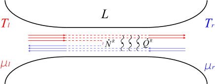
Figure 1: (Color online) Schematic picture of a quantum wire of length $L$. Electrons in the left and right leads are described by Fermi distribution functions characterized by temperatures $T_{l(r)}$ and chemical potentials $\mu_{l(r)}$. Due to three-particle collisions electrons may backscatter and also exchange energy between the subsystems of warmer right movers and colder left movers.

II.2 Partially equilibrated electrons

We start our discussion of the different scattering processes involved in the electronic relaxation with the process shown in Fig. 2(a). This three-particle collision provides intra-branch relaxation within the subsystem of right-moving electrons. A similar relaxation process for the left movers is not shown in the figure but is implicit. This process can be described by the corresponding inelastic scattering length, which we denote in the following as $\ell_{a}$. The precise form of $\ell_{a}$ and its temperature dependence are model specific. They are determined by the scattering amplitude for the given interaction potential and the phase space available for this scattering [Fig. 2(a)] to occur. Quite generally one may argue that $\ell_{a}$ scales as a power of $T$. Indeed, at low temperatures, $T\ll\mu$, all participating scattering states are located within the energy strip $\sim T$ near the Fermi level. What is important for the present discussion is that for wires with length $L\gg\ell_{a}$ intrabranch electron collisions [Fig. 2(a)] become so efficient that the initial distribution function Eq. (4) will be modified by interactions. One can find the resulting distribution by employing the following observation. Intrabranch collisions conserve independently six quantities. These are the number of right and left movers, $N^{R/L}=\sum_{p\gtrless 0}f_{p}$, their momenta, $P^{R/L}=\sum_{p\gtrless 0}pf_{p}$, and energies, $E^{R/L}=\sum_{p\gtrless 0}\varepsilon_{p}f_{p}$. The form of the resulting electron distribution function $f_{p}$ can be obtained from a general statistical mechanics argument by maximizing the entropy of electrons, $S=-\sum_{p}[f_{p}\ln f_{p}+(1-f_{p})\ln(1-f_{p})]$, under the constraint of the conserved quantities TJK

$$f_{p}=\frac{\theta(p)}{e^{\frac{\varepsilon_{p}-pu^{R}-\mu^{R}}{\mathcal{T}^{R}}}+1}+\frac{\theta(-p)}{e^{\frac{\varepsilon_{p}-pu^{L}-\mu^{L}}{\mathcal{T}^{L}}}+1}\,.$$ (5)

This distribution is characterized by six unknown parameters (Lagrange multipliers) which have a transparent physical interpretation. Indeed, in Eq. (5) $\mathcal{T}^{R/L}$ are effective electron temperatures for right and left movers different from those in the leads. The parameters $u^{R/L}$ have dimension of velocity and account for the conservation of momentum in electron collisions. Finally, $\mu^{L/R}$ are unequilibrated chemical potentials of left- and right-moving particles. In principle, all these parameters may depend on the position along the wire.

For longer wires interbranch three-particle collisions [see Fig. 2(b)] become progressively more important. Unlike intrabranch relaxation these processes allow energy and momentum exchange between the subsystems of right and left movers; thus $P^{R/L}$ and $E^{R/L}$ are no longer independently conserved. However, the full momentum $P=P^{R}+P^{L}$ and energy $E=E^{R}+E^{L}$ are obviously conserved. Corresponding to Fig. 2(b), the scattering length $\ell_{b}$ is model specific and calculated in Appendix C. We note here that for all interaction potentials we studied $\ell_{b}/\ell_{a}\sim\mu/T\gg 1$. In view of this distinct length scale separation, $\ell_{b}\gg\ell_{a}$, the electron distribution in Eq. (5) is established at the first stage of the thermalization process. However, for longer wires, $L\gg\ell_{b}$, relaxation of counterpropagating electrons becomes so efficient that the temperatures $\mathcal{T}^{R/L}$ and boost velocities $u^{R/L}$ of right and left movers become equal, $\mathcal{T}^{R}=\mathcal{T}^{L}=\mathcal{T}$ and $u^{R}=u^{L}=u$, due to energy and momentum exchange. At the same time, the chemical potentials $\mu^{R/L}$ are still unequilibrated in this regime, $\Delta\mu=\mu^{R}-\mu^{L}\neq 0$, since the numbers of right- and left-moving electrons are still independently conserved. As a result, for wires with length $L\gg\ell_{b}$ the distribution function (5) transforms into

$$f_{p}=\frac{\theta(p)}{e^{\frac{\varepsilon_{p}-pu-\mu^{R}}{\mathcal{T}}}+1}+\frac{\theta(-p)}{e^{\frac{\varepsilon_{p}-pu-\mu^{L}}{\mathcal{T}}}+1}\,.$$ (6)

Because $\Delta\mu\neq 0$ we refer to the states of electron system described by the distributions in Eqs. (5) and (6) as the states of partial equilibration.

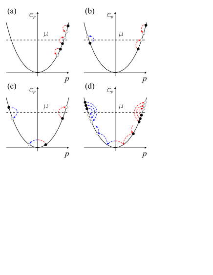
Figure 2: (Color online) (a) Intra-branch relaxation of co-moving electrons that establishes the partially equilibrated form of the distribution function in Eq. (5). (b) Dominant interbranch three-particle process for the energy exchange $\dot{Q}^{R}$ between counterpropagating electrons that contributes to the thermal conductance correction. (c) Leading three-particle collision which results in a finite rate $\dot{N}^{R}\propto e^{-\mu/T}$ and thus a temperature-dependent correction to the conductance of a short wire (Ref. Lunde, ). (d) Equilibration mechanism: multistep diffusion through the bottom of the band of an electron from the right to the left Fermi point accompanied by the excitation of many electron-hole pairs (Refs. JTK, ; TJK, ; ATJK, ).

II.3 Fully equilibrated electrons

Energy and momentum conservation allow for the scattering process in which an electron at the bottom of the band is backscattered by two other particles near the Fermi level [see Fig. 2(c)]. This is the basic three-particle process that changes the numbers of right and left movers before and after collision. In particular, the exponentially small discontinuity of the distributions Eqs. (5) and (6) at $p=0$ will be smeared by collisions of this type.

Complete equilibration of electrons, namely, relaxation of $\Delta\mu$, relies on the electron backscattering from the right to the left Fermi point. One should notice here that it is impossible to realize such scattering directly since it requires momentum transfer of $2p_{F}$ while Fermi blocking restricts typical momentum exchange in the collision to $\delta p\sim T/v_{F}\ll p_{F}$. As a consequence, complete electron backscattering, and thus relaxation of the chemical potential difference $\Delta\mu$, occurs via a large number of small steps $\delta p$ in momentum space such that $\delta p\ll p_{F}$. JTK In its passage between the subsystems of right and left movers the backscattered electron has to pass the bottleneck of occupied states at the bottom of the band [see Fig. 2(d)]. As a result, backscattering of electrons is exponentially suppressed by the probability $\sim e^{-\mu/T}$ to find an unoccupied state at the bottom of the band, and thus the equilibration length $\ell_{eq}$ for the relaxation of the difference in chemical potentials of left and right movers is exponentially large, $\ell_{eq}\propto e^{\mu/T}$. For sufficiently long wires, $L\gg\ell_{eq}$, the state of full equilibration is achieved and described by the distribution JTK ; TJK

$$f_{p}=\frac{1}{e^{\frac{\varepsilon_{p}-v_{d}p-\mu_{eq}}{\mathcal{T}}}+1}\,,$$ (7)

where the chemical potential $\mu_{eq}$ inside the equilibrated wire is, in general, different from $\mu_{l(r)}$ in the leads. In Eq. (7) $v_{d}=I/ne$ is the electron drift velocity, where $I$ is the electric current and $n$ is the electron density. The partially equilibrated distribution function given by Eq. (6) smoothly interpolates to the state of full equilibration, Eq. (7), when the length of the wire exceeds the equilibration length $\ell_{eq}$. The fully equilibrated distribution Eq. (7) is obtained from Eq. (6) by setting $\mu^{R}=\mu^{L}=\mu_{eq}$; thus $\Delta\mu=0$, and also $u=v_{d}$.

II.4 Brief summary

The regime of partial equilibration described by the distribution function in Eq. (6) covers a wide range of lengths, $\ell_{a}\ll L\lesssim\ell_{eq}$. It is more likely to be realized in experiments than the fully equilibrated regime (7), as the length scale $\ell_{eq}$ is exponentially large. Depending on the wire length $L$ a particular state of the electron system is characterized by the extent to which the difference in chemical potentials $\Delta\mu$ and temperatures $\Delta T$ of left and right movers has relaxed. The recent works Refs. TJK, ; ATJK, addressed transport properties of wires with lengths in the range

$$\ell_{a}\ll\ell_{b}\ll L\sim\ell_{eq},$$ (8)

which covers the crossover from the partially equilibrated regime Eq. (6) to the fully equilibrated regime Eq. (7). The major emphasis of these works was on the effect of equilibration due to electron backscattering [Fig. 2(d)]. The main focus of the present paper is on the transport properties of partially equilibrated wires with length

$$\ell_{a}\ll L\sim\ell_{b}\ll\ell_{eq}.$$ (9)

In this regime the numbers $N^{L}$ and $N^{R}$ of the left- and right-moving electrons are individually conserved up to corrections as small as $e^{-\mu/T}$, so that electrons with energies near the Fermi level pass through the wire without backscattering [Fig. 2(c)]. This automatically implies that the conductance $G$ unchaged intact by interactions and is still given by Eq. (2). However, electrons will experience other multiple three-particle collisions [Fig. 2(b)], which allow momentum and energy exchange within and between the two branches of the spectrum, thus altering thermal transport properties. The role of these processes was not explored in previous studies devoted to the transport in partially equilibrated quantum wires. TJK ; ATJK

III Boltzmann equation formalism

III.1 Three-particle collision integral

Consider a quantum wire of length $L$, connected by ideal reflectionless contacts to noninteracting leads which are biased by a temperature difference $\Delta T$ (see Fig. 1). In the following, we are interested only in the thermal transport properties of the wire and assume that there is no external voltage bias, $V=0$. We describe weakly interacting one-dimensional electrons in the framework of the Boltzmann kinetic equation

$$v_{p}\partial_{x}f(p,x)=\mathcal{I}\{f(p,x)\}\,,$$ (10)

where $v_{p}=p/m$ is the electron velocity and the evolution of the distribution function is governed by the collision integral $\mathcal{I}\{f(p,x)\}$. We consider the steady-state setup in which the distribution function does not depend explicitly on time. The collision integral, in general, is a nonlinear functional of $f(p,x)$, whose form is determined by the scattering processes affecting the distribution function. As discussed above, in our case the dominant processes are three-particle collisions. Assuming that the collision integral is local in space, we have

$$\mathcal{I}\{f_{1}\} = -\hskip-11.38092pt\sum_{p_{2},p_{3}\atop p_{1^{\prime}},p_{2^{\prime}},p_{3^{\prime}}}\!\!\!W^{1^{\prime}2^{\prime}3^{\prime}}_{123}$$ (11)

$$\times\left[f_{1}f_{2}f_{3}(1-f_{1^{\prime}})(1-f_{2^{\prime}})(1-f_{3^{\prime}})\right.$$

$$\left.-f_{1^{\prime}}f_{2^{\prime}}f_{3^{\prime}}(1-f_{1})(1-f_{2})(1-f_{3})\right],$$

where $W^{1^{\prime}2^{\prime}3^{\prime}}_{123}$ is the scattering rate from the incoming states $\{p_{1},p_{2},p_{3}\}$ into the outgoing states $\{p_{1^{\prime}},p_{2^{\prime}},p_{3^{\prime}}\}$, and we used the shorthand notation $f_{i}=f(p_{i},x)$. The Boltzmann equation [Eq. (10)] is supplemented by the boundary conditions stating that the distribution $f(p,0)$ of right-moving electrons ($p>0$) at the left end of the wire and $f(p,L)$ of left-moving electrons ($p<0$) at the right end coincide with the distribution function in the leads, Eq. (4). We note here that although Eq. (11) is written for the spinless case our subsequent analysis and solution of the Boltzmann equation presented in Sec. III.2–III.4 is applicable to the spinful electrons as well.

An exact analytical solution of the Boltzmann equation [Eq. (10)] is, in general, very difficult to find due to the nonlinearity of the collision integral Eq. (11). A simplification is, however, possible in the case of a linear response analysis in the externally applied perturbation (in our case, the temperature difference $\Delta T$). Then the collision integral can be linearized near its unperturbed value. It is convenient to present $f(p,x)$ as

$$f(p,x)=f^{0}_{p}+f^{0}_{p}(1-f^{0}_{p})\psi(p,x)\,,$$ (12)

where $f^{0}_{p}=(e^{(\varepsilon_{p}-\mu)/T}+1)^{-1}$ is the equilibrium Fermi distribution function and $\psi(p,x)\propto\Delta T$. When linearizing Eq. (11) with respect to $\psi(p,x)$ the factor $f^{0}_{p}(1-f^{0}_{p})$ in Eq. (12) makes it convenient to use the detailed balance condition

$$f^{0}_{p_{1}}f^{0}_{p_{2}}f^{0}_{p_{3}}(1-f^{0}_{p_{1^{\prime}}})(1-f^{0}_{p_{2^{\prime}}})(1-f^{0}_{p_{3^{\prime}}})=$$

$$f^{0}_{p_{1^{\prime}}}f^{0}_{p_{2^{\prime}}}f^{0}_{p_{3^{\prime}}}(1-f^{0}_{p_{1}})(1-f^{0}_{p_{2}})(1-f^{0}_{p_{3}})\,,$$ (13)

valid at $\varepsilon_{p_{1}}+\varepsilon_{p_{2}}+\varepsilon_{p_{3}}=\varepsilon_{p_{1^{\prime}}}+\varepsilon_{p_{2^{\prime}}}+\varepsilon_{p_{3^{\prime}}}$. Substituting Eq. (12) into the collision integral and using Eq. (III.1) one arrives at the linearized version of Eq. (11)

$$\!\!\!\!\!\mathcal{I}\{\psi(p_{1},x)\}\! = \!-\!\!\!\!\!\sum_{p_{2},p_{3}\atop p_{1^{\prime}},p_{2^{\prime}},p_{3^{\prime}}}\!\!\!\mathbb{K}^{1^{\prime}2^{\prime}3^{\prime}}_{123}$$ (14)

$$\!\!\!\times\left[\psi(p_{1},x)+\psi(p_{2},x)+\psi(p_{3},x)\right.$$

$$\!\!\!\left.-\psi(p_{1^{\prime}},x)-\psi(p_{2^{\prime}},x)-\psi(p_{3^{\prime}},x)\right]\,,$$

with the kernel $\mathbb{K}$ defined as

$$\mathbb{K}^{1^{\prime}2^{\prime}3^{\prime}}_{123} = W^{1^{\prime}2^{\prime}3^{\prime}}_{123}f^{0}_{p_{1}}f^{0}_{p_{2}}f^{0}_{p_{3}}$$ (15)

$$\times(1-f^{0}_{p_{1^{\prime}}})(1-f^{0}_{p_{2^{\prime}}})(1-f^{0}_{p_{3^{\prime}}})\,.$$

The explicit form of the scattering rate $W^{1^{\prime}2^{\prime}3^{\prime}}_{123}$ is not important for the following discussion. It is discussed in detail in Appendix B.

III.2 Solution strategy

Even after linearization the solution of the integral Boltzmann equation that satisfies given boundary conditions is still a complicated problem. However, our task is simplified greatly since we already know the structure of the distribution function $f(p,x)$. Indeed, we have discussed in Sec. II that for wires with length $\ell_{a}\ll L\sim\ell_{b}$ the electron system is in the regime of partial equilibration with the distribution function given by Eq. (5). Thus, the class of functions we need to consider to solve our boundary problem is, in fact, rather narrow. The solution we are seeking is conveniently parametrized by six unknowns: $\mu^{R(L)}(x)$, $u^{R(L)}(x)$, and $\mathcal{T}^{R(L)}(x)$. Instead of solving one integro-differential equation for $f(p,x)$ we will reduce our task to solving a system of six linear ordinary differential equations that govern the spatial evolution of the parameters defining the distribution function in Eq. (5). This is possible since the momentum dependence of the distribution function is fully determined by our ansatz (5), which allows completion of all $p$ integrations in the Boltzmann equation analytically. Among the six equations we need, four represent conservation laws: conservation of numbers of right- and left-moving electrons $N^{R/L}$, of total momentum $P$, and of energy $E$ of the electron system. The other two are kinetic equations that account for the momentum and energy exchange between subsystems of right and left movers, thus capturing the processes of thermalization.

For the following analysis it is convenient to measure the chemical potentials and temperatures from their equilibrium values: $\mu^{R(L)}(x)=\mu+\delta\mu^{R(L)}(x)$ and $\mathcal{T}^{R(L)}(x)=T+\delta\mathcal{T}^{R(L)}(x)$. Expanding now Eq. (5) to the linear order in $u^{R(L)}$, $\delta\mu^{R(L)}$ and $\delta\mathcal{T}^{R(L)}$ and using Eq. (12) we can identify $\psi(p,x)$ that enters the collision integral in Eq. (14) as

$$\psi(p,x)=\psi^{R}(p,x)+\psi^{L}(p,x)$$ (16)

where

$$\hskip-15.6491pt\psi^{R(L)}(p,x)=\theta(\pm p)$$

$$\hskip-15.6491pt\times\left[\psi^{R(L)}_{\mu}(p,x)+\psi^{R(L)}_{u}(p,x)+\psi^{R(L)}_{\mathcal{T}}(p,x)\right].$$ (17)

Here the three contributions are

$$\psi^{R(L)}_{\mu}(p,x)=\frac{\delta\mu^{R(L)}(x)}{T}\,,$$ (18)

$$\psi^{R(L)}_{u}(p,x)=\frac{pu^{R(L)}(x)}{T}\,,$$ (19)

$$\psi^{R(L)}_{\mathcal{T}}(p,x)=\frac{(\varepsilon_{p}-\mu)\delta\mathcal{T}^{R(L)}(x)}{T^{2}}\,.$$ (20)

These functions evolve in the real space as prescribed by the collision integral Eq. (14) while their boundary values can be extracted from the respective distributions in the leads [Eq. (4)]. Indeed, expanding Eq. (4) with $V=0$ one obtains

$$f_{p}=f^{0}_{p}+\frac{(\varepsilon_{p}-\mu)\Delta T}{2T^{2}}f^{0}_{p}(1-f^{0}_{p})[\theta(p)-\theta(-p)].$$ (21)

By matching this result to Eq. (12) with $\psi(p,x)$ taken from Eqs. (16) and (III.2) we deduce the boundary conditions

$$\delta\mu^{R}(0)=\delta\mu^{L}(L)=0\,,$$ (22)

$$u^{R}(0)=u^{L}(L)=0\,,$$ (23)

$$\delta\mathcal{T}^{R}(0)=-\delta\mathcal{T}^{L}(L)=\Delta T/2\,.$$ (24)

Our task now is to derive the set of coupled ordinary differential equations that govern the spatial evolution of the unknown parameters $u^{R(L)}(x)$, $\delta\mu^{R(L)}(x)$, and $\delta\mathcal{T}^{R(L)}(x)$. This will give us complete knowledge of the electron distribution function. Knowing all parameters in Eq. (5) we will be able to find the heat current and finally the thermal conductance of the system. Before we realize this plan, the conservation laws must be discussed.

III.3 Transport currents and conservation laws

Conservation of the total number of particles implies that in a steady state the particle current $I(x)$ is uniform along the wire. Correspondingly, we infer from the conservation of total momentum $P$ and total energy $E$ that in the steady state a constant momentum current $I_{P}$ and a constant energy current $I_{E}$ flow through the system. In the following it will be convenient to express these currents as the sums of individual contributions of the left- and right-moving electrons, e.g., $I=I^{R}+I^{L}$, thus introducing:

$$\hskip-14.22636ptI^{R(L)}(x)=\int^{+\infty}_{-\infty}\frac{dp}{h}\,\theta(\pm p)v_{p}f(p,x)\,,$$ (25)

$$\hskip-14.22636ptI^{R(L)}_{P}(x)=\int^{+\infty}_{-\infty}\frac{dp}{h}\,\theta(\pm p)pv_{p}f(p,x)\,,$$ (26)

$$\hskip-14.22636ptI^{R(L)}_{E}(x)=\int^{+\infty}_{-\infty}\frac{dp}{h}\,\theta(\pm p)\varepsilon_{p}v_{p}f(p,x)\,.$$ (27)

The positive sign in the step function corresponds to right movers and the negative one to left movers. Since we neglect small backscattering effects, the numbers of right- and left-moving electrons are conserved independently:

$$\dot{N}^{R/L}=0\,.$$ (28)

It follows then immediately from the continuity equations that particle currents are uniform along the wire,

$$\partial_{x}I^{R}(x)=0\,,\qquad\partial_{x}I^{L}(x)=0\,.$$ (29)

Similarly we present the conservation of total momentum and energy,

$$\partial_{x}\big{[}I^{R}_{P}(x)+I^{L}_{P}(x)\big{]}=0\,,$$ (30)

$$\partial_{x}\big{[}I^{R}_{E}(x)+I^{L}_{E}(x)\big{]}=0\,.$$ (31)

As the next step we express the currents (25)–(27) in terms of the parameters defining the electron distribution function. Specifically, we use Eq. (12) and Eqs. (III.2)–(20) together with the current definition in Eq. (25) and thus find from Eq. (29)

$$\frac{d\delta\mu^{R(L)}}{dx}=\mp p_{F}\frac{du^{R(L)}}{dx}\left(1-\frac{\pi^{2}T^{2}}{24\mu^{2}}-\frac{7\pi^{4}T^{4}}{384\mu^{4}}\right)\,.$$ (32)

When deriving this equation from Eq. (25) we had to carry out a Sommerfeld expansion up to the fourth order in $T/\mu\ll 1$. Note here that even though backscattering is neglected $\delta\mu^{R(L)}$ must change in space to accommodate the conservation laws for currents [Eqs. (29)–(31)], and $\mu^{R(L)}(x)=\mu+\delta\mu^{R(L)}(x)$ coincide with $\mu_{r(l)}=\mu$ only at the ends of the wire [see the boundary conditions Eq. (22)].

We then perform a similar calculation for the momentum and energy currents. From the momentum conservation Eq. (30), we find

$$p_{F}\frac{T}{2\mu}\left(1+\frac{5\pi^{2}}{12}\frac{T^{2}}{\mu^{2}}\right)\left(\frac{du^{R}}{dx}-\frac{du^{L}}{dx}\right)+$$

$$\left(1+\frac{7\pi^{2}}{40}\frac{T^{2}}{\mu^{2}}\right)\left(\frac{d\delta\mathcal{T}^{R}}{dx}+\frac{d\delta\mathcal{T}^{L}}{dx}\right)=0\,,$$ (33)

while from the energy conservation, Eq. (31),

$$p_{F}\frac{T}{2\mu}\left(1+\frac{7\pi^{2}}{40}\frac{T^{2}}{\mu^{2}}\right)\left(\frac{du^{R}}{dx}+\frac{du^{L}}{dx}\right)+$$

$$\left(\frac{d\delta\mathcal{T}^{R}}{dx}-\frac{d\delta\mathcal{T}^{L}}{dx}\right)=0\,.$$ (34)

When deriving these two equations we also made use of Eq. (32) to exclude the chemical potentials of the right and left movers.

III.4 Scattering processes and kinetic equations

Although the total momentum and energy currents $I_{P}$ and $I_{E}$ are conserved, such currents taken for the left and right movers separately, $I^{R/L}_{P}$ and $I^{R/L}_{E}$, are not. Indeed, the three-particle collisions shown in Fig. 2(b) induce momentum and energy exchange between counter-propagating electrons. Let us focus on a small segment of the wire between the positions $x$ and $x+\Delta x$, where $0<x<L$. The difference $I^{R/L}_{P}(x+\Delta x)-I^{R/L}_{P}(x)$ is equal to the rate of change of the momentum of right-moving electrons $\dot{P}^{R/L}=\dot{p}^{R/L}\Delta x$. Here $\dot{p}^{R/L}$ is the rate per unit of length. As a result, the continuity equation for the momentum exchange reads

$$\partial_{x}\big{[}I^{R}_{P}(x)-I^{L}_{P}(x)\big{]}=2\dot{p}^{R}\,.$$ (35)

Here we used $\dot{p}^{L}=-\dot{p}^{R}$, which is ensured by the conservation of total momentum. In complete analogy we can now relate the difference of energy currents $I^{R}_{E}(x+\Delta x)-I^{R}_{E}(x)$ to the corresponding energy exchange rate $\dot{E}^{R}=\dot{e}^{R}\Delta x$, which gives us

$$\partial_{x}\big{[}I^{R}_{E}(x)-I^{R}_{E}(x)\big{]}=2\dot{e}^{R}\,,$$ (36)

where we also used $\dot{e}^{L}=-\dot{e}^{R}$ guaranteed by the energy conservation. The right-hand side of Eqs. (35) and (36) can be calculated from the collision integral of the Boltzmann equation [Eq. (14)].

There are two basic processes which contribute to $\dot{p}^{R}$ and $\dot{e}^{R}$. The first one includes two right movers that scatter off one left mover. This process is shown in Fig. 2(d). The other process, when two left movers scatter off one right mover, is equally important. Keeping both terms, using Eqs. (14) and (16) we find for the relaxation rates (details of the derivation are given in Appendix A)

$$\hskip-19.91684pt\dot{p}^{R}=-k_{F}\frac{p_{F}}{2\tau}\frac{u^{R}-u^{L}}{v_{F}}\,,$$ (37)

$$\hskip-19.91684pt\dot{e}^{R}=-k_{F}\frac{\mu}{\tau}\frac{\delta\mathcal{T}^{R}-\delta\mathcal{T}^{L}}{T}\,,$$ (38)

$$\hskip-19.91684pt\frac{1}{\tau}=\frac{3}{k_{F}\Delta x}\sum_{p_{1}>0,p_{2}>0,p_{3}<0\atop p_{1^{\prime}}>0,p_{2^{\prime}}>0,p_{3^{\prime}}<0}\frac{v^{2}_{F}(p_{3^{\prime}}-p_{3})^{2}}{\mu T}\mathbb{K}^{1^{\prime}2^{\prime}3^{\prime}}_{123}.$$ (39)

Having determined relaxation the rates we now return to Eqs. (35) and (36). Computing the momentum and energy currents of right and left movers in the same way as we did in the previous section from Eqs. (26)–(27) and using the relaxation rates from Eqs. (37)–(38) we find two additional equations which describe the relaxation of momentum:

$$p_{F}\frac{\pi^{2}T^{2}}{12\mu^{2}}\!\left(\frac{du^{R}}{dx}+\frac{du^{L}}{dx}\right)\!\!\left(1+\frac{5\pi^{2}}{12}\frac{T^{2}}{\mu^{2}}\right)$$

$$+\frac{\pi^{2}T}{6\mu}\!\left(\frac{d\delta\mathcal{T}^{R}}{dx}-\frac{d\delta\mathcal{T}^{R}}{dx}\right)\!\!\left(1+\frac{7\pi^{2}}{40}\frac{T^{2}}{\mu^{2}}\right)$$

$$=\!-\frac{hk_{F}}{\tau}\frac{u^{R}-u^{L}}{v_{F}}$$ (40)

and energy

$$\hskip-14.22636ptp_{F}\frac{\pi^{2}T^{2}}{6\mu^{2}}\left(\frac{du^{R}}{dx}-\frac{du^{L}}{dx}\right)\!\!\left(1+\frac{7\pi^{2}}{40}\frac{T^{2}}{\mu^{2}}\right)+$$

$$\hskip-14.22636pt\frac{\pi^{2}T}{3\mu}\!\left(\frac{d\delta\mathcal{T}^{R}}{dx}+\frac{d\delta\mathcal{T}^{L}}{dx}\right)\!=-\frac{2hk_{F}}{\tau}\frac{\delta\mathcal{T}^{R}-\delta\mathcal{T}^{L}}{T}.$$ (41)

Equations (32)–(III.3) and (III.4)–(III.4), together with the boundary conditions Eqs. (22)–(24), represent the closed system of six coupled differential equations whose solution fully determines the six parameters $\mu^{R/L},u^{R/L},\mathcal{T}^{R/L}$ that define the electron distribution function (5). We now find these parameters explicitly. For that purpose let us introduce dimensionless variables

$$\eta_{\pm}=\frac{u^{R}\pm u^{L}}{v_{F}}\,,\qquad\theta_{\pm}=\frac{\delta\mathcal{T}^{R}\pm\delta\mathcal{T}^{L}}{T}\,,$$ (42)

and the microscopic scattering length

$$\ell_{b}=\frac{\pi^{3}T^{4}}{360\mu^{4}}(v_{F}\tau)\,.$$ (43)

Calculation of $\ell_{b}$ requires a detailed knowledge of the scattering rate, implicit in the kernel $\mathbb{K}^{1^{\prime}2^{\prime}3^{\prime}}_{123}$, as a function of momenta transferred in a collision. In Appendix B we provide this information for the case of the three-particle collisions under consideration and in Appendix C find $\ell_{b}$ explicitly for the spinless and spinful cases.

After some algebra the coupled equations (III.3), (III.3) and (III.4), (III.4) can be reduced to the following form:

$$\frac{\partial\theta_{+}}{\partial x}=-\alpha\frac{\partial\eta_{-}}{\partial x}\,,$$ (44)

$$\frac{\partial\eta_{+}}{\partial x}=-\beta\frac{\partial\theta_{-}}{\partial x}\,,$$ (45)

$$\frac{\partial\theta_{-}}{\partial x}=\frac{\eta_{-}}{\ell_{b}}\,,$$ (46)

$$\frac{\partial\eta_{-}}{\partial x}=\frac{\theta_{-}}{\ell_{b}}\,,$$ (47)

which contain two dimensionless parameters

$$\alpha=1+\frac{29\pi^{2}}{120}\frac{T^{2}}{\mu^{2}}\,,\quad\beta=1-\frac{7\pi^{2}}{40}\frac{T^{2}}{\mu^{2}}\,,$$ (48)

where corrections of higher order in $T/\mu\ll 1$ were neglected. The remaining two equations for the chemical potentials of right and left movers [Eq. (32)] are not written here for brevity. The latter do not enter the heat current and thus are not explicitly needed. Equations (44)–(47) can now be easily solved, with the result

$$\theta^{R}(x)=\frac{\Delta T}{2T}\frac{\alpha_{-}e^{x/\ell_{b}}+\alpha_{+}e^{(L-x)/\ell_{b}}}{\alpha_{-}+\alpha_{+}e^{L/\ell_{b}}}\,,$$ (49)

$$\theta^{L}(x)=-\frac{\Delta T}{2T}\frac{\alpha_{+}e^{x/\ell_{b}}+\alpha_{-}e^{(L-x)/\ell_{b}}}{\alpha_{-}+\alpha_{+}e^{L/\ell_{b}}}\,,$$ (50)

$$\eta^{R}(x)=\frac{\Delta T}{2T}\frac{\beta_{-}(e^{x/\ell_{b}}-1)-\beta_{+}(e^{(L-x)/\ell_{b}}-e^{L/\ell_{b}})}{\alpha_{-}+\alpha_{+}e^{L/\ell_{b}}}\,,$$ (51)

$$\eta^{L}(x)=-\frac{\Delta T}{2T}\frac{\beta_{+}(e^{x/\ell_{b}}-e^{L/\ell_{b}})-\beta_{-}(e^{(L-x)/\ell_{b}}-1)}{\alpha_{-}+\alpha_{+}e^{L/\ell_{b}}}\,,$$ (52)

where $\alpha_{\pm}=1\pm\alpha$, $\beta_{\pm}=1\pm\beta$ and $\theta^{R/L}=(\theta_{+}\pm\theta_{-})/2$, $\eta^{R/L}=(\eta_{+}\pm\eta_{-})/2$. This concludes our solution of the Boltzmann equation for three-particle collisions.

IV Heat current and thermal conductance

Complete knowledge of the distribution function (5) allows us to compute physical observables. Specifically, we are interested in the thermal conductance $K$. For the latter we need to evaluate the heat current

$$I_{Q}(x)=I_{E}(x)-\mu I(x)\,.$$ (53)

By using Eqs. (5) we carry out a Sommerfeld expansion for the particle and energy currents $I$ and $I_{E}$ from Eqs. (25) and (27), up to the fourth order in $T/\mu\ll 1$, and then find from the above definition [Eq. (53)]

$$I_{Q}(x)=\frac{\pi^{2}T^{2}}{3h}\left[\frac{\eta_{+}(x)}{\beta}+\theta_{-}(x)\right],$$ (54)

which is presented here in our notation defined in Eq. (42). With the help of Eqs. (49)–(52) it can be readily checked that $I_{Q}$ is uniform along the wire. This fact is a priori expected and follows from the conservation laws, which we already explored above. By knowing $I_{Q}$ we can finally find the thermal conductance $K(L)=I_{Q}/\Delta T$ as a function of the wire length,

$$\frac{K(L)}{K_{0}}=\frac{\tanh(L/2\ell_{b})+\beta}{\alpha\beta\tanh(L/2\ell_{b})+\beta}\,.$$ (55)

This is the main result of our paper. Note here that $K_{0}=\pi^{2}T/3h$ for the case of spinless electrons, whereas $K_{0}$ is given by Eq. (3) for electrons with spin. The functional form of $K(L)$ remains the same in both cases except for the expressions for $\ell_{b}$, which we discuss below. Let us now analyze limiting cases of Eq. (55) and discuss the microscopic form of the scattering length $\ell_{b}$.

Equation (55) interpolates smoothly between two distinct limits. In short wires, $L\ll\ell_{b}$, from the expansion of Eq. (55) one obtains for the interaction-induced correction to thermal conductance, $\delta K=K-K_{0}$, the following result:

$$\frac{\delta K(L)}{K_{0}}=-\frac{\pi^{2}}{30}\frac{T^{2}}{\mu^{2}}\frac{L}{\ell_{b}}\,,\quad L\ll\ell_{b}\,.$$ (56)

In such short wires electrons propagate from one lead to the other, rarely experiencing three-particle collisions of the type shown in Fig. 2(b). Thus their distribution function is approximately determined by that in the leads [Eq. (4)]. Under this assumption one can adopt the strategy of Ref. Lunde, , applied previously for the calculation of conductance and thermopower in short wires, and treat the collision integral of the Boltzmann equation perturbatively, thus neglecting effects of thermalization on the distribution function. Technically speaking, this corresponds to a lowest order iteration for the Boltzmann equation, which amounts to substituting distribution (4) into the collision integral (14) to calculate the correction to $I_{Q}$. This perturbative procedure immediately reproduces Eq. (56).

It is physically expected that in longer wires particle collisions Fig. 2(b) should have a much more dramatic effect on the distribution function and thus thermal transport. Indeed, once full thermalization has been achieved for $L\gg\ell_{b}$ we find from Eq. (55) that the correction to thermal conductance saturates:

$$\frac{\delta K(L)}{K_{0}}=-\frac{\pi^{2}}{30}\frac{T^{2}}{\mu^{2}}\,,\quad\ell_{b}\ll L\ll\ell_{eq}\,.$$ (57)

One interesting aspect of Eq. (57) is that $\delta K$ is independent of the interaction strength. It means that no matter how weak the interactions are, for sufficiently long wires thermalization between right- and left-moving electrons is eventually established, which leads to saturation of $\delta K$. The behavior of $\delta K(L)$ as a function of the wire length is summarized Fig. 3.

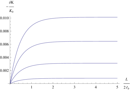
Figure 3: (Color online) Interaction-induced correction to the thermal conductance of a clean quantum wire as a function of its length plotted for different values of temperature (from the bottom to the top curve): $T/\mu=0.05,0.1,0.15,0.2$. For $L\ll\ell_{b}$ the correction scales with $L$ and saturates to a constant value $\propto\left(T/\mu\right)^{2}$ once $\ell_{b}\ll L$ in accordance with Eqs. (56) and (57).

The interaction strength, however, sets the length scale $\ell_{b}$ at which thermalization occurs. Its actual dependence on temperature is determined by the phase space available for a three-particle collision to occur and by the dependence of the corresponding scattering amplitude on momenta transferred in a collision. For spinless electrons and Coulomb interaction we find (see Appendix C for the derivation and additional discussions)

$$\ell^{-1}_{b}\simeq k_{F}\lambda_{1}(k_{F}w)(e^{2}/\hbar v_{F}\kappa)^{4}(T/\mu)^{3}\,,$$ (58)

where $w$ is thw wire width and $\lambda_{1}(z)=z^{4}\ln^{2}(1/z)$. In the case of spinful electrons, the scattering length changes to

$$\ell^{-1}_{b}\simeq k_{F}\lambda_{2}(k_{F}w)(e^{2}/\hbar v_{F}\kappa)^{4}(T/\mu)\ln^{2}(\mu/T)\,,$$ (59)

where $\lambda_{2}(z)=\ln^{2}(1/z)$. Contrasting Eqs. (58) and (59), one sees that the spin of the electron plays an important role since the inverse scattering length of spinful electrons is significantly larger, by a factor of $(\mu/T)^{2}\gg 1$. This is a manifestation of the Pauli exclusion principle. Indeed, for three-particle scattering to occur electrons must approach each other on a distance of the order of $\sim k^{-1}_{F}$. When electrons are spinless the Pauli exclusion suppresses the probability of such scattering. In contrast, the suppression is not as strong when the total spin of the three colliding particles is $1/2$ since at least two electrons may have opposite spins while exclusion applies to the third particle. This technical point and the importance of the exchange effect in the scattering amplitudes are discussed in more detail in Appendix B.

V Discussion

In this paper we studied the thermal transport properties of one-dimensional electrons in quantum wires. In this system equilibration is strongly restricted by the phase space available for electron scattering and conservation laws such that leading effects stem from the three-particle collisions. This is in sharp contrast with higher-dimensional systems where already pair collisions provide electronic relaxation. Although our theory is applicable only in the weakly interacting limit, the results presented are still beyond the picture of the Luttinger liquid since three-particle collisions are not captured by the latter. We have elucidated the microscopic processes involved in electron thermalization and developed a scheme for solving the Boltzmann equation analytically within a linear response analysis. Our approach allows us to find the thermal conductance for arbitrary relations between the wire length and microscopic relaxation length [see Eq. (55)].

In order to establish a connection to previous work TJK ; ATJK we emphasize that our solution of the kinetic equations and the result for thermal conductance presented in Eq. (55) rely on the simplifying assumption that electron backscattering can be neglected. This is a good approximation except for the case of very long wires, $L\gtrsim\ell_{eq}$, where the small probability of backscattering $\sim e^{-\mu/T}$ is compensated by the large phase space available for scattering to happen. Accounting for the backscattering processes, it was found in Ref. TJK, that for wires with length $L\sim\ell_{eq}$ the thermal conductance is

$$\frac{K(L)}{K_{0}}=\frac{\ell_{eq}}{L+\ell_{eq}}\,.$$ (60)

This result gives only an exponentially small correction to the thermal conductance, $\delta K/K_{0}=-L/\ell_{eq}\propto e^{-\mu/T}$, in the limit $L\ll\ell_{eq}$, since in the analysis of Ref. TJK, thermalization effects on the distribution function were neglected. It is our result Eq. (57) that gives the leading-order correction to $\delta K$ in this case. On the other hand, our expression (55) is not applicable for the long wires, $L\sim\ell_{eq}$, whereas Eq. (60) works in this regime. It displays an essentially different feature, which is solely due to backscattering processes, namely, the vanishing thermal conductance $\delta K\propto 1/L$ as $L\to\infty$.

Our work may be relevant for a number of recent experiments. In particular, the authors of Ref. Chiatti, reported thermal conductance measurements and a lower value of $K$ than that predicted by the Wiedemann-Franz law, at the plateau of electrical conductance. As we explained, corrections to $G$ are exponentially small, $G=2e^{2}/h-\mathcal{O}(e^{-\mu/T})$, for wires with $L\ll\ell_{eq}$. Thus the conductance remains essentially unaffected by interactions, and its quantization is robust. In contrast, the effect of three-particle collisions on the thermal conductance is much more pronounced. Our equation (57) shows that the thermal conductance is reduced by interactions, which is qualitatively consistent with the experimental observation. Chiatti Apparent violation of the Wiedemann-Franz law is due to the fact that interaction-induced corrections $\delta K$ and $\delta G$ originate from physically distinct scattering processes [see Figs. 2(b) and 2(c), respectively].

Another experiment Birge reported measurements of the electron distribution function in one-dimensional wires. This experiment demonstrated that electrons thermalize despite the severe constraints imposed by the conservation laws and dimensionality on the particle collisions. We take the point of view that three-particle collisions are responsible for relaxation and provide an explicit solution of the Boltzmann equation, thus uncovering the structure of the distribution function [see Eqs. (5) and (49)–(52)], which in principle can be compared to experimental results. Estimate

A related study Barak provided us information about the time scales of thermalization of one-dimensional electrons. Although we do not study the latter our results for the relaxation lengths Eqs. (58) and (59) can be directly linked to the experiment. Note also that the dramatic difference between the relaxation lengths, and thus the times, of spinful and spinless electrons provides a distinct signature of three-particle collisions that could be tested experimentally.

There is a very important limitation on the applicability of Eqs. (55) and (59) that we need to discuss in the case of spinful electrons. KOG From the point of view of Luttinger liquid theory, electrons are not well-defined excitations in one dimension and instead one should use a bosonic description in terms of charge and spin modes. The weakly interacting limit considered here and usage of the Boltzmann equation assumes that electrons maintain their integrity during collisions and thus neglects effects of spin-charge separation. In order to quantify to what extent such a description is valid, consider an electron with excitation energy $\xi$ above the Fermi energy $\mu$. For quadratic dispersion, $\varepsilon_{p}=p^{2}/2m$, the velocity of such electrons differs from that of the electrons in the Fermi sea by an amount $\Delta v=\xi/mv_{F}$. Spin and charge do not separate appreciably if $\Delta v\gg v_{c}-v_{s}$, where $v_{c(s)}$ are the velocities of charge (spin) excitations. At finite temperatures the characteristic excitation energy is $\xi\sim T$, so that the above condition can be equivalently reformulated as $T/\mu\gg(v_{c}-v_{s})/v_{F}$. For weakly interacting electrons the difference between the velocities of charge and spin modes is related to the zero-momentum Fourier component of the electron-electron interaction potential, namely, $v_{c}-v_{s}\simeq V_{0}/\pi\hbar\ll 1$. This implies that at low temperatures when $T/\mu\ll V_{0}/\hbar v_{F}$ a description in terms of electrons breaks down and Eqs. (55) and (59) are no longer applicable.

Finally, our work also points to open issues and directions for future research. It is of great interest to understand the fate of energy relaxation and the nature of thermal transport in the case of strong interactions which simultaneously have to be combined with nonequilibrium conditions. At very low temperatures a description of a one-dimensional system in terms of electronic excitations becomes inadequate even if the interactions are weak. The effect of spin-charge separation has to be included, and thermal transport from plasmons and their relaxation are central issues to consider.

Acknowledgements

We would like to acknowledge useful discussions with A. V. Andreev, N. Andrei, N. Birge, P. W. Brouwer, L. I. Glazman, A. Imambekov, A. Kamenev, T. Karzig, and F. von Oppen. This work at ANL was supported by the U.S. DOE, Office of Science, under Contract No. DE-AC02-06CH11357, and at ENS by the ANR Grant No. 09-BLAN-0097-01/2 (Z.R.).

Appendix A Derivation of $\dot{P}^{R}$ and $\dot{E}^{R}$

In this appendix we derive Eqs. (37)–(39) presented in the main text of the paper. As explained in Sec. III.4, when computing $\dot{P}^{R}$ and $\dot{E}^{R}$ we have to account for two types of scattering process. One is shown in Fig. 2(b) and the other is similar and consists of a scattering of one left mover and two right movers. We start by considering the quantity $\mathcal{P}_{n}=\sum_{p_{1}>0}p_{1}^{n}f_{1}$. Its rate of change is

$$\dot{\mathcal{P}}_{n} =\sum_{p_{1}>0}p_{1}^{n}\dot{f}_{1}=-\sum_{p_{1}>0,p_{2},p_{3}\atop p_{1^{\prime}},p_{2^{\prime}},p_{3^{\prime}}}p_{1}^{n}\mathbb{K}^{1^{\prime}2^{\prime}3^{\prime}}_{123}$$

$$\times\left(\psi_{1}+\psi_{2}+\psi_{3}-\psi_{1^{\prime}}-\psi_{2^{\prime}}-\psi_{3^{\prime}}\right),$$ (61)

where we used the Boltzmann equation [Eq. (10)] and the short-hand notation $\psi_{i}=\psi(p_{i},x)$. It is convenient to split each sum from the last equation into parts that contain positive and negative values of the momenta, so that one gets

$$\dot{\mathcal{P}}_{n}=\sum_{+--\atop---}(\ldots)+3\sum_{+--\atop++-}(\ldots)+6\sum_{++-\atop+--}(\ldots)+\sum_{+--\atop+++}(\ldots)$$

$$+\sum_{+++\atop---}(\ldots)+3\sum_{+++\atop+--}(\ldots)+3\sum_{+++\atop++-}(\ldots)+2\sum_{++-\atop+++}(\ldots)$$

$$+2\sum_{++-\atop---}(\ldots)+3\sum_{+--\atop+--}(\ldots)+6\sum_{++-\atop++-}(\ldots)+\sum_{+++\atop+++}(\ldots).$$ (62)

The notations here are as follows

$$\sum_{+--\atop---}(\ldots)=\sum_{p_{1}>0,p_{2}<0,p_{3}<0\atop p_{1^{\prime}}<0,p_{2^{\prime}}<0,p_{3^{\prime}}<0}(\ldots)\,,$$ (63)

and analogously for the other terms. When deriving Eq. (A) we have used the following symmetry properties of the kernel: (a) exchange of incoming and outgoing momenta $\mathbb{K}_{123}^{1^{\prime}2^{\prime}3^{\prime}}=\mathbb{K}_{1^{\prime}2^{\prime}3^{\prime}}^{123}$, (b) pairwise exchange $\mathbb{K}_{123}^{1^{\prime}2^{\prime}3^{\prime}}=\mathbb{K}_{213}^{2^{\prime}1^{\prime}3^{\prime}}$, and (c) inversion of momenta $p_{i}\to-p_{i}$, $\mathbb{K}_{123}^{1^{\prime}2^{\prime}3^{\prime}}=\mathbb{K}_{-1-2-3}^{-1^{\prime}-2^{\prime}-3^{\prime}}$. In the final expression for $\dot{\mathcal{P}}_{n}$ we keep only the terms of Eq. (A) that contain equal numbers of positive incoming and outgoing momenta, i.e., the last three terms. The other terms contain at least one state near the bottom of the band and therefore give a contribution that is exponentially suppressed due to the small probability of finding an unoccupied state. After employing Eqs. (16)–(20) combined with momentum and energy conservations, we end up with

$$\dot{\mathcal{P}}_{n}\!\! =\!\! 3\sum_{++-\atop++-}\mathbb{K}_{123}^{1^{\prime}2^{\prime}3^{\prime}}\bigg{[}\frac{\delta\mathcal{T}^{R}-\delta\mathcal{T}^{L}}{T^{2}}\left[2p_{1}^{n}-(-p_{3})^{n}\right]$$

$$\times \!\!\!(\varepsilon_{p_{3}}-\varepsilon_{p_{3^{\prime}}})+\frac{u^{L}-u^{R}}{T}\left[2p_{1}^{n}+(-p_{3})^{n}\right](p_{3}-p_{3^{\prime}})\bigg{]}.$$

For $n=1$ from the last expression we easily get

$$\dot{P}^{R}=\dot{\mathcal{P}}_{1}=-3\frac{u^{R}-u^{L}}{T}\sum_{++-\atop++-}\mathbb{K}_{123}^{1^{\prime}2^{\prime}3^{\prime}}(p_{3^{\prime}}-p_{3})^{2},$$ (64)

which reduces to Eq. (37) in the main text. For $n=2$

$$\dot{E}^{R}=\frac{\dot{\mathcal{P}}_{2}}{2m}=-3\frac{\delta\mathcal{T}^{R}-\delta\mathcal{T}^{L}}{T^{2}}\sum_{++-\atop++-}\mathbb{K}_{123}^{1^{\prime}2^{\prime}3^{\prime}}(\varepsilon_{p_{3^{\prime}}}-\varepsilon_{p_{3}})^{2}\,.$$ (65)

One additional step is required to obtain Eq. (38). Since all three particles participating in a collision are located near the Fermi points it means that the characteristic momentum of right movers is $\sim p_{F}$ while for the left mover it is $\sim-p_{F}$. In contrast, the momenta transferred in a collision $q_{i}=p_{i^{\prime}}-p_{i}$ are much smaller $\sim T/v_{F}\ll p_{F}$, which stems from the temperature smearing of the occupation functions implicit in the kernel $\mathbb{K}^{1^{\prime}2^{\prime}3^{\prime}}_{123}$. Since $|q_{i}|\ll p_{F}$ we approximate $p_{3}\approx-p_{F}$ and linearize the spectrum near the Fermi points, in particular,

$$\varepsilon_{p_{3}+q_{3}}-\varepsilon_{p_{3}}\approx\frac{1}{2m}[(-p_{F}+q_{3})^{2}-p^{2}_{F}]\approx-v_{F}q_{3}\,,$$ (66)

which then brings the last expression for $\dot{E}^{R}$ to the form of Eq. (38) in the main text.

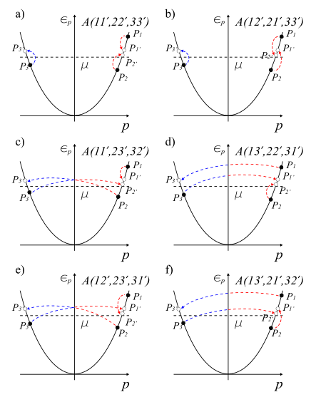
Figure 4: (Color online) Direct (a) and five exchange (b)–(f) terms in the three-particle amplitude $\mathcal{A}^{1^{\prime}2^{\prime}3^{\prime}}_{123}$ [Eq. (68)] that contribute to the finite momentum $\dot{P}^{R}$ and energy $\dot{E}^{R}$ exchange rates between right and left movers.

Appendix B Three-particle scattering amplitude

For most of our analysis the detailed form of the scattering rate entering kinetic equation (10) was not important. However, for the calculation of the microscopic quantities, such as the scattering lengths $\ell_{a}$ and $\ell_{b}$, we need to know the precise form of the scattering rate $W^{1^{\prime}2^{\prime}3^{\prime}}_{123}$ introduced in Eq. (11). Below we give the details of the structure of the scattering rate. We start with the golden rule expression

$$W^{1^{\prime}2^{\prime}3^{\prime}}_{123}=\frac{2\pi}{\hbar}|\mathcal{A}^{1^{\prime}2^{\prime}3^{\prime}}_{123}|^{2}\delta(E-E^{\prime})\delta_{P,P^{\prime}}$$ (67)

where $\mathcal{A}^{1^{\prime}2^{\prime}3^{\prime}}_{123}$ is the corresponding scattering amplitude, while the $\delta$-functions impose conservations of the total energy $E(E^{\prime})=\sum_{i}\varepsilon_{p_{i}(p_{i^{\prime}})}$ and total momentum $P(P^{\prime})=\sum_{i}p_{i(i^{\prime})}$ of the colliding electrons. One should note that in Eq. (67) we include $\delta_{P,P^{\prime}}$ in the definition of the scattering rate $W^{1^{\prime}2^{\prime}3^{\prime}}_{123}$ rather than the amplitude $\mathcal{A}^{1^{\prime}2^{\prime}3^{\prime}}_{123}$, which is in contrast to the usual convention. This step simplifies our notations.

Since the electrons interact with two-particle interaction potential $V(x)$, the three-particle scattering amplitude is found to the second order in $V(x)$. The details of this calculation were presented in Ref. Lunde, . In the case of spinless electrons the final result reads

$$\mathcal{A}^{1^{\prime}2^{\prime}3^{\prime}}_{123}=\sum_{\pi(1^{\prime}2^{\prime}3^{\prime})}\mathrm{sgn}(1^{\prime}2^{\prime}3^{\prime})A(11^{\prime},22^{\prime},33^{\prime})\,.$$ (68)

One should notice that Eq. (68) contains the term $A(11^{\prime},22^{\prime},33^{\prime})$, which is the amplitude of the direct scattering process [Fig. 4(a)], and the terms obtained by the remaining five permutations of the outgoing momenta, which are the exchange terms [Figs. 4(b)–4(f)]. They can be written compactly for the segment $\Delta x$ of the wire as follows:

$$A(1a,2b,3c) = a^{ab}_{12}+a^{ac}_{13}+a^{bc}_{23}\,,$$ (69)

$$a^{ab}_{12} \equiv a^{p_{a}p_{b}}_{p_{1}p_{2}}=\frac{1}{(\Delta x)^{2}}V_{p_{a}-p_{1}}V_{p_{b}-p_{2}}$$ (70)

$$\times \left[\frac{1}{E\!-\!\varepsilon_{p_{1}}\!-\!\varepsilon_{p_{b}}\!-\!\varepsilon_{P-p_{1}-p_{b}}}\right.$$

$$+ \left.\frac{1}{E\!-\!\varepsilon_{p_{a}}\!-\!\varepsilon_{p_{2}}\!-\!\varepsilon_{P-p_{a}-p_{2}}}\right],$$

where $(a,b,c)$ is a particular permutation of $(1^{\prime},2^{\prime},3^{\prime})$. In Eq. (68) the notations $\pi(\ldots)$ and $\mathrm{sgn}(\ldots)$ denote permutations of the final momenta and parities of a particular permutation. Finally, $V_{p}$ is the Fourier-transformed component of the bare two-body interaction potential. For the calculations we take the Coulomb interaction between electrons,

$$V(x)=\frac{e^{2}}{\kappa}\left[\frac{1}{\sqrt{x^{2}+4w^{2}}}-\frac{1}{\sqrt{x^{2}+4d^{2}}}\right]\,,$$ (71)

screened by a nearby gate, which we model by a conducting plane at a distance $d$ from the wire. We also introduced a small width $w$ of the quantum wire, $w\ll d$, to regularize the diverging short-range behavior of this potential. This enables us to evaluate the small-momentum Fourier components $V_{p}$ of the interaction potential $V(x)$. To this end, we find in the limit $\hbar/d\ll p\ll\hbar/w$

$$V_{p}={2e^{2}\over\kappa}\ln\left(\frac{p_{w}}{|p|}\right)\left[1+\frac{p^{2}}{p^{2}_{w}}\right]\,,$$ (72)

while in the limit of very small momenta $p\ll\hbar/d$

$$V_{p}=\frac{2e^{2}}{\kappa}\ln\left(\frac{d}{w}\right)\left[1-\frac{p^{2}}{p^{2}_{d}}\frac{\ln(p_{d}/|p|)}{\ln(d/w)}\right]\,.$$ (73)

In the last two equations we introduced the notations $p_{w}=\hbar/w$ and $p_{d}=\hbar/d$. We also employed logarithmic accuracy approximation for $V_{p}$, meaning that numerical coefficients in the arguments of the logarithms in Eqs. (72) and (73) are neglected. In the following discussions we refer to Eq. (72) as the unscreened Coulomb potential and to Eq. (73) as the screened one. The complete expression for the amplitude (68) with the interaction potential taken in the form (72) or (73) is fairly complicated. However, major simplification is possible by studying the kinematics of the three-particle collisions, which in a way allows us to obtain the approximated form of the amplitude for specific scattering processes, such as the one in Fig. 2(b), which determines the scale $\ell_{b}$.

It is convenient to label the outgoing momenta as $p_{i^{\prime}}=p_{i}+q_{i}$ for $i=1,2,3$ in order to separate explicitly the momenta $q_{i}$ transferred in a collision. Momentum conservation then reads

$$q_{1}+q_{2}+q_{3}=0\,.$$ (74)

while energy conservation $E=E^{\prime}$ can be equivalently rewritten as

$$2p_{1}q_{1}+2p_{2}q_{2}+2p_{3}q_{3}+q^{2}_{1}+q^{2}_{2}+q^{2}_{3}=0\,.$$ (75)

At low temperatures, $T\ll\mu$, the Fermi occupation functions constrain particles participating in the collision to lie in a momentum strip of the order of $T/v_{F}\ll p_{F}$ near the Fermi level. This means in practice that the typical momentum transferred in a collision will not exceed $\mathrm{max}\{|q|\}\lesssim T/v_{F}$. To leading order in $T/\mu\ll 1$ the energy and momentum conservation requirements for the scattering process in Fig. 4 can be resolved by

$$q_{1}\approx-q_{2}+\mathcal{O}\{[(p_{1}-p_{2}),q_{2}]/p_{F}\}\,,$$ (76a)

and

$$q_{3}\approx\frac{q_{1}(q_{1}+p_{1}-p_{2})}{2p_{F}}+\mathcal{O}\{[(p_{1}-p_{2}),q_{1}]^{2}/p^{2}_{F}\}\,,$$ (76b)

where we used $p_{1}-p_{2}\sim T/v_{F}$ and set $p_{3}\approx-p_{F}$. From this analysis one concludes that energy transfer between the right and left movers occurs via small portions of momentum $q_{3}$ exchange such that

$$\{|q_{1}|,|q_{2}|\}\sim T/v_{F}\,,\quad|q_{3}|\sim T^{2}/v_{F}\mu\ll\{|q_{1}|,|q_{2}|\}\,.$$ (77)

Having two small parameters at hand, $|q_{1}|/p_{F}\ll 1$ and $|q_{3}|/|q_{1}|\ll 1$, and accounting for all the exchange contributions, one can expand the amplitude (68) to the leading nonvanishing order.ZAK In the course of this expansion we observed that exchange contributions result in severe cancellations between different scattering processes. The result of the calculations for the model of unscreened interaction (72) is

$$|\mathcal{A}^{1^{\prime}2^{\prime}3^{\prime}}_{123}|^{2}=\left(\frac{2e^{2}}{\kappa}\right)^{4}\!\!\frac{9\lambda_{1}(k_{F}w)}{64\mu^{2}(\Delta x)^{4}}\ln^{2}\left(\frac{q^{2}_{1}}{2p_{F}|q_{3}|}\right)$$ (78)

where the amplitude is written for a segment of the wire of length $\Delta x$ and the function $\lambda_{1}(k_{F}w)$ was introduced earlier [see the definition after Eq. (58)]. For the screened case we find

$$\hskip-11.38092pt|\mathcal{A}^{1^{\prime}2^{\prime}3^{\prime}}_{123}|^{2}\!\! = \!\!\left(\frac{2e^{2}}{\kappa}\right)^{4}\!\!\frac{25\lambda_{3}(k_{F}d)}{4\mu^{2}(\Delta x)^{4}}$$ (79)

$$\times \!\!\left[\frac{q^{2}_{1}}{p^{2}_{F}}\ln\left(\frac{p_{F}}{|q_{1}|}\right)-\frac{4q^{2}_{3}}{q^{2}_{1}}\ln\left(\frac{|q_{1}|}{|q_{3}|}\right)\right]^{2},$$

where $\lambda_{3}(z)=z^{8}\ln^{2}(1/z)$. Both amplitudes (78) and (79) are written in logarithmic accuracy approximation. As argued above, the typical scattering processes studied here involve only small-momentum transfer, of the order of $q\sim T/v_{F}$. As a result, from the conditions of applicability of the interaction potential Eq. (72) it follows that the corresponding amplitude Eq. (78) applies for $T\gg\hbar v_{F}/d$. Similarly, the screened interaction potential Eq. (73) and corresponding amplitude Eq. (79) apply at lower temperatures $T\ll\hbar v_{F}/d$.

There are several general remarks we need to make regarding the scattering amplitude in Eq. (68). It is known from the context of integrable quantum many-body problems Sutherland that for some two-body potentials, $N$-body scattering processes factorize into a sequence of two-body collisions. In the context of this work, this means that three-particle scattering for the integrable potentials may result only in permutations within the group of three momenta of the colliding particles; all other three-particle scattering amplitudes must be exactly zero for such potentials. We have checked explicitly that the three-particle scattering amplitude in Eq. (68) is nullified for several special potentials: for the contact interaction, $V_{p}=\mathrm{const}$, for the Calogero-Suthreland model, $V_{p}\propto|p|$, and also for the potential $V_{p}\propto 1-p^{2}/p^{2}_{0}$ which is dual to the bosonic Lieb-Liniger model. Surprisingly, we have also noticed that the logarithmic interaction potential $V_{p}\propto\ln|p|$ gives exactly zero for the three-particle amplitude in Eq. (68) although we are unaware of any exactly solvable model for that case. This is the reason to keep the next leading-order term $\sim(p/p_{w})^{2}\ll 1$ in Eq. (72), which prevents the amplitude in Eq. (68) from vanishing exactly.

The second set of remarks concern electrons with spin. For the latter the three-particle amplitude has the same form as Eq. (68), but it acquires an additional dependence on the spin indices:

$$\mathcal{A}^{1^{\prime}2^{\prime}3^{\prime}}_{123}=\!\!\!\!\sum_{\pi(1^{\prime}2^{\prime}3^{\prime})}\!\!\!\mathrm{sign}(1^{\prime}2^{\prime}3^{\prime})\Xi^{\sigma_{1}\sigma_{2}\sigma_{3}}_{\sigma_{1^{\prime}}\sigma_{2^{\prime}}\sigma_{3^{\prime}}}A(11^{\prime},22^{\prime},33^{\prime}),$$ (80)

where $\Xi^{\sigma_{1}\sigma_{2}\sigma_{3}}_{\sigma_{1^{\prime}}\sigma_{2^{\prime}}\sigma_{3^{\prime}}}=\delta_{\sigma_{1}\sigma_{1^{\prime}}}\delta_{\sigma_{2}\sigma_{2^{\prime}}}\delta_{\sigma_{3}\sigma_{3^{\prime}}}$. One can repeat the expansion of the amplitude for $|q_{1}|/p_{F}\ll 1$ and $|q_{3}|/|q_{1}|\ll 1$ and observe that due to the spin structure the exchange terms do not cancel each other. In particular, with the help of Eq. (72) we find the amplitude for the case of the unscreened Coulomb potential in the form

$$\!\sum_{\{\sigma\}}\!|\mathcal{A}^{1^{\prime}2^{\prime}3^{\prime}}_{123}|^{2}\!\!=\!\left(\frac{2e^{2}}{\kappa}\right)^{\!4}\!\!\!\frac{3\lambda_{2}(k_{F}w)}{32\mu^{2}(\Delta x)^{4}}\!\!\left[\frac{4p^{2}_{F}}{q^{2}_{1}}+\frac{q^{2}_{1}}{q^{2}_{3}}\right]\!\ln^{2}\!\!\left(\!\frac{2p_{F}}{|q_{1}|}\!\right),$$ (81)

which is by a factor of $(p_{F}/|q_{1}|)^{2}\gg 1$ larger than Eq. (78); $\lambda_{2}(k_{F}w)$ was defined under Eq. (59).

Appendix C Intra-branch and inter-branch relaxation lengths

In this appendix we estimate the scattering lengths $\ell_{a}$ and $\ell_{b}$. Our starting point for evaluation of the inter-branch length $\ell_{b}$ is the expression

$$\ell^{-1}_{b}=\frac{1080\mu^{4}}{\pi^{3}T^{4}}\frac{1}{v_{F}k_{F}\Delta x}\sum_{++-\atop++-}\frac{(v_{F}q_{3})^{2}}{\mu T}W^{1^{\prime}2^{\prime}3^{\prime}}_{123}\mathbb{F}\{f^{0}\},$$ (82)

which follows from Eqs. (39) and (43), where in addition we introduced the notation

$$\mathbb{F}\{f^{0}\}=f^{0}_{p_{1}}(1-f^{0}_{p_{1}+q_{1}})f^{0}_{p_{2}}(1-f^{0}_{p_{2}+q_{2}})f^{0}_{p_{3}}(1-f^{0}_{p_{3}+q_{3}}).$$ (83)

In view of the kinematic constraints (76a) and (76b), conservation of momentum and energy in the expression (67) for the scattering rate $W^{1^{\prime}2^{\prime}3^{\prime}}_{123}$ can be presented as

$$\delta(E-E^{\prime})\delta_{P,P^{\prime}}\approx\frac{1}{2v_{F}}\delta\left(q_{3}-\frac{q_{1}(q_{1}+p_{1}-p_{2})}{2p_{F}}\right)\delta_{q_{1},-q_{2}},$$ (84)

which eliminates two out of six momentum integrations in Eq. (82). The other four integrals can be completed analytically with logarithmic accuracy. This amounts to replacing the weak logarithmic parts of the amplitude in Eqs. (78), (79), and (81) by their typical values taken at characteristic momenta $q_{1}\sim T/v_{F}$ and $q_{3}\sim T^{2}/v_{F}\mu$. We thus treat $\ln(q^{2}_{1}/2p_{F}|q_{3}|)$ in Eq. (78) as a constant of order unity and approximate $\ln(p_{F}/|q_{1}|)\simeq\ln(|q_{1}|/|q_{3}|)\simeq\ln(\mu/T)$ in Eqs. (79) and (81). After this step we can integrate in Eq. (82) explicitly by linearizing the electron dispersion relation inside the Fermi functions and get

$$\hskip-28.45274pt\sum_{p_{1}p_{2}p_{3}}\!\!q^{4}_{1}\mathbb{F}\{f^{0}\}=\frac{(\Delta x)^{3}T}{4h^{3}v_{F}}\frac{q^{6}_{1}}{\sinh^{2}\left(\frac{v_{F}q_{1}}{2T}\right)},$$ (85)

$$\hskip-28.45274pt\sum_{p_{1}p_{2}p_{3}}\!\!q^{3}_{1}(p_{1}-p_{2})\mathbb{F}\{f^{0}\}=-\frac{(\Delta x)^{3}T}{4h^{3}v_{F}}\frac{q^{6}_{1}}{\sinh^{2}\left(\frac{v_{F}q_{1}}{2T}\right)},$$ (86)

$$\hskip-28.45274pt\sum_{p_{1}p_{2}p_{3}}\!\!q^{2}_{1}(p_{1}-p_{2})^{2}\mathbb{F}\{f^{0}\}=\frac{(\Delta x)^{3}T}{6h^{3}v_{F}}\frac{q^{4}_{1}\left(\frac{7q^{2}_{1}}{4}+\frac{\pi^{2}T^{2}}{v^{2}_{F}}\right)}{\sinh^{2}\left(\frac{v_{F}q_{1}}{2T}\right)}.$$ (87)

For the spinless case and high-temperature regime $T\gg\hbar v_{F}/d$, where the Coulomb interaction is unscreened, we obtain

$$\ell^{-1}_{b}\simeq\frac{\lambda_{1}(k_{F}w)}{p^{2}_{F}T^{4}\Delta x}\left(\frac{e^{2}}{\hbar\kappa}\right)^{4}\sum_{q_{1}}\frac{q^{4}_{1}\left(\frac{q^{2}_{1}}{4}+\frac{\pi^{2}T^{2}}{v^{2}_{F}}\right)}{\sinh^{2}\left(\frac{v_{F}q_{1}}{2T}\right)}.$$ (88)

Note here that we do not keep track of the numerical coefficient in the expression for $\ell_{b}$ since within the adopted calculation with logarithmic accuracy this coefficient is not determined. After the remaining $q_{1}$ integration one recovers Eq. (58), presented in the main text of the paper.

At lower temperatures $T\ll\hbar v_{F}/d$, screening effects become important and one should use Eq. (79) in the expression for the scattering length Eq. (82). Estimation of $\ell_{b}$ in this case gives

$$\ell^{-1}_{b}\simeq k_{F}\lambda_{3}(k_{F}d)(e^{2}/\hbar v_{F}\kappa)^{4}(T/\mu)^{7}\ln^{2}(\mu/T)\,.$$ (89)

In the spinful case this calculation is completely analogous to the one above; we just need to use a different expression for the scattering amplitude. With the help of Eq. (81), which is applicable for the model of an unscreened Coulomb potential interaction, we get at the intermediate step with logarithmic accuracy,

$$\ell^{-1}_{b}\simeq\frac{\lambda_{2}(k_{F}w)}{T^{4}\Delta x}\left(\frac{e^{2}}{\hbar\kappa}\right)^{4}\!\!\ln^{2}\left(\frac{\mu}{T}\right)\sum_{q_{1}}\frac{q^{2}_{1}\left(\frac{5q^{2}_{1}}{2}+\frac{4\pi^{2}T^{2}}{v^{2}_{F}}\right)}{\sinh^{2}\left(\frac{v_{F}q_{1}}{2T}\right)}.$$ (90)

After the final integration this translates into Eq. (59).

We turn now to discussion of the intra-branch relaxation length $\ell_{a}$ introduced in Sec. II. Unlike the case of interbranch relaxation, Fig. 1(b), here all three colliding particles are near the same Fermi point; see Fig. 1(a). In this case, the typical momentum change for the three electrons is the same,

$$|q_{1}|\sim|q_{2}|\sim|q_{3}|\sim T/v_{F}.$$ (91)

At this point we should emphasize that for the processes that determine the length scale $\ell_{b}$, a new energy scale $T^{2}/\mu$ appeared in the problem purely from the kinematic constraints based on the conservation laws. This scale determined the typical momentum transfer of the particle that was alone at one side of the Fermi surface; see Eqs. (76b) and (77).

Another important quantity is the scattering amplitude. For Coulomb interaction and for the process where all three particles are near the same Fermi point, it is a relatively complicated expression, but similarly to Eqs. (78) and (79) it depends on momenta only weakly (logarithmically) for the intra-branch processes.

These two observations help us to estimate $\ell_{a}$ using the known result Eq. (58) for $\ell_{b}$. Namely, by replacing the energy scale $T^{2}/\mu$ in $\ell_{b}$ by $T$, we obtain the estimate

$$\ell^{-1}_{a}\simeq k_{F}\lambda_{1}(k_{F}w)(e^{2}/\hbar v_{F}\kappa)^{4}(T/\mu)^{2},$$ (92)

for the unscreened Coulomb case, $T\gg\hbar v_{F}/d$. At lower temperatures, $T\ll\hbar v_{F}/d$ it changes to $\ell^{-1}_{a}\propto T^{6}$. It is important to emphasize that regardless of the interaction model we use there exists a distinct separation between the scales of the relaxation lengths, namely,

$$\ell_{a}/\ell_{b}\sim T/\mu\ll 1.$$ (93)

This fact justifies our ansatz for the distribution function [see the discussion after Eq. (5)]. The detailed calculation of $\ell_{a}$ will be presented elsewhere. ZAK

References

- (1) A. A. Abrikosov, Fundamentals of the Theory of Metals (North-Holland, Amsterdam, 1988).
- (2) G. V. Chester and A. Thellung, Proc. Phys. Soc. London 77, 1005 (1961).
- (3) Electron-Electron Interaction In Disordered Systems, edited by A. J. Efros and M. Pollak (Elsevier, Amsterdam, 1985).
- (4) G. Catelani and I. L. Aleiner, JETP 100, 331 (2005).
- (5) T. Giamarchi, Quantum Physics in One Dimension, (Claredon Press, Oxford, 2003).
- (6) D. L. Maslov and M. Stone, Phys. Rev. B 52, R5539 (1995); V. V. Ponomarenko, Phys. Rev. B 52, R8666 (1995); I. Safi and H. J. Schulz, Phys. Rev. B 52, R17040 (1995).
- (7) R. Fazio, F. W. J. Hekking, and D. E. Khmelnitskii, Phys. Rev. Lett. 80, 5611 (1998).
- (8) C. L. Kane and M. P. A. Fisher, Phys. Rev. Lett. 68 1220 (1992); 76, 3192 (1996).
- (9) K. Schwab, E. A. Henriksen, J. M. Worlock, and M. L. Roukes, Nature Phys. 404, 974 (2000).
- (10) O. Chiatti, J. T. Nicholls, Y. Y. Proskuryakov, N. Lumpkin, I. Farrer, and D. A. Ritchie, Phys. Rev. Lett. 97, 056601 (2006).
- (11) J. T. Nicholls and O. Chiatti, J. Phys.: Condens. Matter 20, 164210 (2008).
- (12) F. Sfigakis, A. C. Graham, K. J. Thomas, M. Pepper, C. J. B. Ford, and D. A Ritchie, J. Phys.: Condens. Matter 20, 164213 (2008).
- (13) G. Granger, J. P. Eisenstein, and J. L. Reno, Phys. Rev. Lett. 102, 086803 (2009).
- (14) C. Altimiras, H. le Sueur, U. Gennser, A. Cavanna, D. Mailly, and F. Pierre, Nature Phys. 6, 34 (2009).
- (15) Y. F. Chen, T. Dirks, G. Al-Zoubi, N. O. Birge, and N. Mason, Phys. Rev. Lett. 102, 036804 (2009).
- (16) G. Barak, H. Steinberg, L. N. Pfeiffer, K. W. West, L. I. Glazman, F. von Oppen, and A. Yakoby, Nature Phys. 6, 489 (2010).
- (17) D. B. Gutman, Y. Gefen, and A. D. Mirlin, Phys. Rev. Lett. 101, 126802 (2008); Phys. Rev. B 81, 085436 (2010).
- (18) S. Takei, M. Milletari, and B. Rosenow, Phys. Rev. B 82, 041306 (2010).
- (19) A. M. Lunde, K. Flensberg, and L. I. Glazman, Phys. Rev. B 75, 245418 (2007).
- (20) J. Rech, T. Micklitz, and K. A. Matveev, Phys. Rev. Lett. 102, 116402 (2009).
- (21) T. Micklitz, J. Rech, and K. A. Matveev, Phys. Rev. B 81, 115313 (2010).
- (22) A. Levchenko, T. Micklitz, J. Rech, and K. A. Matveev, Phys. Rev. B 82, 115413 (2010).
- (23) K. A. Matveev, A. V. Andreev, and M. Pustilnik, Phys. Rev. Lett. 105, 046401 (2010).
- (24) T. Karzig, L. I. Glazman, and F. von Oppen, Phys. Rev. Lett. 105, 226407 (2010).
- (25) A. Levchenko, Z. Ristivojevic, and T. Micklitz, Phys. Rev. B 83, 041303(R) (2011).
- (26) Y. M. Sirenko, V. Mitin, and P. Vasilopoulos, Phys. Rev. B 50, 4631 (1994).
- (27) To be accurate we point out that for the noninteracting electrons , where the exponentially small term comes from the states at the bottom of the band. At low temperatures and thus all such small contributions are neglected throughout the paper.
- (28) For the estimates we use typical parameters from the experiment of Ref. Birge, . In particular, m/s, m-1, , and nm. This translates into and meV so that for the temperature K the thermal relaxation length [Eq. (59)] is of the order m.
- (29) Z. Ristivojevic, A. Levchenko and K. Matveev, (unpublished).
- (30) B. Sutherland, Beautiful Models (World Scientific, Singapore, 2004), Secs. 1.3–1.5.