Photocentric variability of quasars caused by variations in their inner structure: Consequences for Gaia measurements

Abstract

Context. We study the photocenter position variability caused by variations in the quasar inner structure. We consider the variability in the accretion disk emissivity and torus structure variability caused by the different illumination by the central source. We discuss the possible detection of these effects by Gaia. Observations of the photocenter variability in two AGNs, SDSS J121855+020002 and SDSS J162011+1724327 have been reported and discussed.

Aims. For variations in the quasar inner structure, we explore how much this effect can affect the position determination and whether it can (or not) be detected with the Gaia mission.

Methods. We use models of (a) a relativistic disk, including the perturbation that can increase the brightness of part of the disk, and consequently offset the photocenter position, and (b) a dusty torus that absorbs and re-emits the incoming radiation from the accretion disk (central continuum source). We estimate the value of the photocenter offset caused by these two effects.

Results. We found that perturbations in the inner structure can cause a significant offset to the photocenter. This offset depends on the characteristics of both the perturbation and accretion disk and on the structure of the torus. In the case of the two considered QSOs, the observed photocenter offsets cannot be explained by variations in the accretion disk and other effects should be considered. We discuss the possibility of exploding stars very close to the AGN source, and also that there are two variable sources at the center of these two AGNs that may indicate a binary supermassive black hole system on a kpc (pc) scale.

Conclusions. The Gaia mission seems to be very promising, not only for astrometry, but also for exploring the inner structure of AGNs. We conclude that variations in the quasar inner structure can affect the observed photocenter (by up to several mas). There is a chance to observe such an effect in the case of bright and low-redshift QSOs.

1 Introduction

Gaia is a global astrometric interferometer mission that aims to determine high-precision astrometric parameters for one billion objects with apparent magnitudes in the range 5.6 $\leq V\leq 20$ (see e.g. Perryman et al., 2001; Lindegren, 2008). It is foreseen that 500 000 QSOs (quasi-stellar objects) will be among these objects. These QSOs will be used to construct a dense optical QSO-based celestial reference frame (see Bourda et al., 2010). The relevance of QSOs to the celestial frames compliant to the ICRS, such as the current ICRF2 or the Gaia celestial reference frame, relies on a photocenter position stability at the sub-mas level. Sub-mas accuracy in the measured positions is the goal of Gaia, namely for objects of 12 mag around 0.003 mas, of 15 mag 0.01 mas and 20 mag 0.2 mas (Perryman et al., 2001).

However, QSOs are active galactic nuclei (AGNs) in whose central region different physical processes occur that may cause a variation in the photometric center of the object. According to the standard model of AGNs, the central region of a QSO consists of a SMBH ($10^{7}-10^{10}\ M_{\odot}$) surrounded by an accretion disk (see Sulentic et al., 2000), and a broad emission-line region (BLR). That central region might be surrounded by dust, arranged in a toroidal-like distribution. All these components radiate, and its strength is a function of the geometry of the system, and its orientation relative to the observer. One of the most important properties of AGNs is their flux variability, which may have multiple origins such as variation in the accretion rate, instabilities of the accretion disk around the central black hole, supernova bursts, jet instabilities, and gravitational microlensing (see e.g. Andrei et al., 2009; Shields et al., 2010; Popović et al., 2011).

Taris et al. (2011) reported on the possibility of a correlation between the flux variability and photocenter motion in QSOs, which is a very relevant subject for missions such as Gaia. There are different sources for photocenter variation. It is well-known that the main output of the different structures of an AGN (such as accretion disk, jets, line-emitting regions, torus, etc.) differ in energy, consequently the sizes and position of the emitting regions are ”wavelength dependent”. Opacity effects also explain the frequency-dependent core-shifts in the radio synchrotron emission at the base of relativistic jets (Porcas, 2009), and core shifts (between two radio wavelengths) of up to 1.4 mas have been reported by Kovalev et al. (2008).

As we mentioned above, an AGN has a complex structure, and one can expect that the origin of this variation is caused by the inner structure of this object, as for instance a torus that is illuminated by a varying central continuum may contribute to some photocenter variation. However, variable processes occurring in the accretion disk, such as outburst, and perturbations (see e.g. Jovanović et al., 2010; Popović et al., 2011).

In this paper, we investigate the spectro-photocentric variability of quasars caused by changes in their inner structure. We consider: (a) a perturbation in a relativistic accretion disk around a SMBH, and (b) changes in the pattern of radiation scattered by the dust particles in the surrounding torus caused by the variations in the accretion disk luminosity and dust sublimation radius.

The aims of the paper are: (a) to show how much these effects may contribute to the variability of the photocenter, i.e. to quantify “noise“ and more accurately characterize any resulting error in the position determination; (b) to estimate the possibility of detecting this effect with Gaia mission; and (c) to identify in which QSOs these effects may be dominant.

The paper is organized as follows: in §2 and §3 we present the models and parameters of the accretion disk and dusty torus; in §4 results of our simulations are given for different parameters of both the disk and torus and at different redshifts; in §5, we consider the properties of two quasars in the context of obtained results from our simulations; and in §6, we outline our conclusions.

In this paper, we use a flat cosmological model with the following parameters: $\Omega_{\mathrm{m}}$­ = 0.27, $\Omega_{\mathrm{\Lambda}}=0.73$, and $H_{0}=71$ km s^-1 Mpc^-1.

2 Disk model around SMBH

In the standard model of an AGN accretion disk, accretion occurs via an optically thick and geometrically thin disk. The effective optical depth in the disk is very high and photons are close to thermal equilibrium with electrons (Jovanović & Popović, 2009). The spectrum of thermal radiation emitted from the accretion disk surface depends on its structure and temperature, hence on the distance to the black hole.

An accretion disk around a supermassive black hole at the center of an AGN extends from the radius of a marginally stable orbit $R_{ms}$ to several thousands of gravitational radii. On the basis of radiation emitted in different spectral bands, it can be stratified in several parts (Jovanović & Popović, 2009): a) an innermost part close to the central black hole that emits X-rays and extends from the radius of marginally stable orbit $R_{ms}$ to several tens of gravitational radii; b) a central part ranging from $\sim 100\ R_{g}$ to $\sim 1000\ R_{g}$, which emits UV radiation; and c) an outer part extending from several hundreds to several thousands $R_{g}$, from which the optical emission orriginates (Eracleous & Halpern, 1994, 2003).

Here we consider an optical emission disk. The model is described in our previous papers (see e.g. Popović et al., 2003; Jovanović & Popović, 2009; Jovanović et al., 2010), and here will not be repeated in detail. We model the emission from an accretion disk using numerical simulations based on a ray-tracing method in a Kerr metric (see e.g. Jovanović & Popović, 2009, and references therein). In this method, one divides the image of the disk on the observer’s sky into a number of small elements (pixels), and for each pixel the photon trajectory is traced backward from the observer by following the geodesics in a Kerr space-time. Although this method was developed for studying the X-ray radiation originating from the innermost parts of the disk close to the central black hole (see e.g. Jovanović & Popović, 2008), it can be also successfully applied to the modeling of the UV/optical emission originating from the outer regions of the disk (see e.g. Jovanović et al., 2010).

However, some general relativistic and strong gravitational effects (such as gravitational redshift) are significant only in the innermost regions of the accretion disk, close to its marginally stable orbit. Since the inner radius of the disk is here taken to be $100\ R_{g}$, and it has a small inclination angle, these effects will have a negligible influence on the photocenter displacement. Therefore, we assumed a non-rotating central black hole, such that the Kerr metric reduces to its special Schwarzschild case. In this way, we also included in our simulations some Newtonian and special relativistic phenomena, such as the Doppler effect and relativistic beaming (see Fig. 1 and top left panel of Fig. 2), which cannot be neglected even at such relatively large distances from the central black hole, hence could cause significant displacements of the photocenter from the position obtained by simply averaging the assumed emissivity function of the disk. On the other hand, this method is very convenient for investigating photocenter variability, because the relativistic ray-tracing enables us to calculate for instance the brightness of each pixel in the accretion disk image on the observer’s sky. This disk image can then be used to easily obtain the photocenter position, as we show in the later text.

2.1 The model of a bright spot–like perturbing region

To model a bright spot on the disk, we considered perturbations in the surface emissivity on some region of the disk. Surface emissivity of the disk is usually assumed to vary with radius as a power law (e.g. Popović et al., 2003) $\varepsilon(x,y)=\varepsilon_{0}\cdot r^{a}(x,y),$ where $\varepsilon_{0}$ is an emissivity constant, $a$ is emissivity index, and $(x,y)$ is a position along the disk. We introduce the perturbation in accretion disk emissivity (bright spot) in the form of a two-dimensional circular Gaussian, by modifying its power-law emissivity according to (Jovanović & Popović, 2009)

$$\varepsilon^{\prime}(x,y)=\varepsilon(x,y)\cdot\left({1+\varepsilon_{p}\cdot e^{-\left({\left({\frac{{x-x_{p}}}{{w_{p}}}}\right)^{2}+\left({\frac{{y-y_{p}}}{{w_{p}}}}\right)^{2}}\right)}}\right),$$ (1)

where $\varepsilon^{\prime}(x,y)$ is the modified disk emissivity, $\varepsilon(x,y)$ is the ordinary power-law disk emissivity at the same position $(x,y)$, $\varepsilon_{p}$ is the emissivity of the perturbing region (i.e. the amplitude of the bright spot), $(x_{p},y_{p})$ is the position of the perturbing region with respect to the disk center (expressed in gravitational radii, hereafter denoted by $R_{g}=GM/c$, where $M$ is the mass of the SMBH, and G and c are well known constants) and $w_{p}$ is its width (also in $R_{g}$). A three-dimensional (3D) plot of the above expression for the modified emissivity law is given in Fig. 1.

Figure 1: A 3D plot of modified disk emissivity given by Eq. (1) for $100\ \mathrm{R_{g}}\leq r(x,y)\leq 3000\ \mathrm{R_{g}}$, $q=-1$ and for the following parameters of perturbing region: $\varepsilon_{p}=10$, $x_{p}=2500\ \mathrm{R_{g}}$, $y_{p}=0\ \mathrm{R_{g}}$, and $w_{p}=300\ \mathrm{R_{g}}$.

Owing to relativistic effects, photons emitted from the disk at frequency $\nu_{em}$ will reach observers at infinity at frequency $\nu_{obs}$, and their ratio determines the shift caused by these effects $g=\nu_{obs}/\nu_{em}$. The total observed flux at the observed energy $E_{obs}$ is then given by

$$F\left({E_{obs}}\right)={\int\limits_{image}{\varepsilon^{\prime}(x,y)}}\,g^{4}\delta\left({E_{obs}-gE_{0}}\right)d\Xi,$$ (2)

where $\varepsilon^{\prime}\left({r}\right)$ is the modified disk emissivity given by Eq. (1), $d\Xi$ is the solid angle subtended by the disk in the observer’s sky, and $E_{0}$ is the rest energy.

This simple model is suitable for our purpose because it allows us to change the amplitude, width, and location of bright spots with respect to the disk center. In this way, we are able to simulate the displacement of a bright spot along the disk, and its widening and amplitude variations with time.

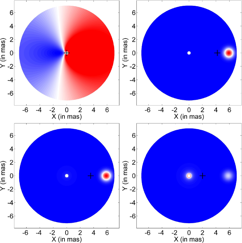
Figure 2: Simulations of the accretion disk without (top left) and with perturbation for three different values of emissivity index: $a=0$ (top right), $a=-1$ (bottom left), and $a=-2$ (bottom right). The photocenter positions are denoted by crosses. In the top left panel, color represents the energy shift due to relativistic effects (i.e. ratio of the observed to emitted energy), while in the other three panels it represents the observed flux (in arbitrary units). The inner and outer radii of the disk, as well as the position and width of the perturbing region, are the same as in Fig. 1. The maximum emissivity of the perturbing region is taken to be ten times greater than the emissivity of the disk at its inner radius. Linear distances are converted to angular units along the $x$ and $y$ axes assuming an accretion disk located at cosmological redshift $z=0.01$ around the central black hole with mass of 10${}^{10}\ M_{\odot}$.

Table 1: The simulated offsets of photocenter (in mas) caused by perturbation to the accretion disk emissivity for different values of its redshift and mass of a central black hole. Other parameters correspond to the bottom left panel of Fig. 2.

$M_{BH}$	$z$
$(M_{\odot})$	0.01	0.05	0.10	0.15	0.20
108	0.036	0.007	0.004	0.003	0.002
109	0.355	0.074	0.039	0.028	0.022
1010	3.550	0.744	0.394	0.278	0.220

2.2 Modeled offset of the photocenter caused by a perturbation (bright spot) in the disk

The observed photocenter $(X_{pc},Y_{pc})$ of the accretion disk can be modeled as a centroid of observed flux $F(E_{obs})$ over the disk image, i.e. as the mean of impact parameters $(x,y)$ of all pixels along the disk image, weighted by $F$

$$X_{pc}=\frac{\sum_{i=1}^{N}\sum_{j=1}^{N}F(i,j)\cdot x(i,j)}{\sum_{i=1}^{N}\sum_{j=1}^{N}F(i,j)},$$

$$Y_{pc}=\frac{\sum_{i=1}^{N}\sum_{j=1}^{N}F(i,j)\cdot y(i,j)}{\sum_{i=1}^{N}\sum_{j=1}^{N}F(i,j)},$$ (3)

where $(i,j)$ is a point on a $N\times N$ grid of the disk image pixels.

We consider a perturbation (or bright spot) at a certain part of the disk, for different values of the spot brightness, and calculate the photocenter. In Fig. 2, we present simulations of the photocenter variability.

2.3 Parameters of the disk and perturbation (bright spot)

In the model, we are able to change the parameters of the accretion disk (dimension, emissivity, inner and outer radius, inclination) and the parameters of the perturbation (size, position, and brightness). Taking into account the results of previous studies, one can expect the dimensions of the accretion disk to be several thousands of gravitational radii (see e.g. Eracleous & Halpern, 1994, 2003; Popović et al., 2011), hence here we assume an accretion disk with an inner and outer radius of R_inn = 100 R_g and R_out=3000 R_g, respectively. In our simulation, we consider a low-inclined ($i=5^{\circ}$) or near face-on disk, because of from investigations of the broad line shapes a near face-on disk is preferred (see e.g. Popović et al., 2004; Bon et al., 2009a). Although the adopted inclination angle is small, it is sufficient to induce Doppler and relativistic beaming effects (see e.g. Fig. 9 in Reynolds & Nowak, 2003, and the corresponding discussion below). As shown in Reynolds & Nowak (2003), even in the case of a nearly face-on disk, these effects can still produce rather broad emission lines, unlike the case of a face-on Newtonian disk, which would display very narrow lines. In addition, for a steep disk emissivity where $a<-2$, the line emission of the disk is dominated by its inner regions $R_{out}<50\ R_{g}$. However, for the disk emissivity where $a>-2$, the bulk of the line emission comes from the outer regions of the disk, thus both Doppler and relativistic beaming effects cannot be neglected even at such relatively large distances from the central black hole. Since the most realistic values for the emissivity of the disk are probably between 0 and $-2$ (see e.g. Eracleous & Halpern, 1994, 2003; Popović et al., 2004; Bon et al., 2009b), we modeled the disk emissivity index as $a=0$, $a=-1$, and $a=-2$.

In our simulation, the dimensions of the perturbation (bright spot) is around 100 – 300 gravitational radii (see Jovanović et al., 2010), taking different values for the brightness and position along the disk.

3 Dusty torus model

According to the AGN unification model, the central continuum source is surrounded by the geometrically and optically thick toroidal structure of dust and gas with an equatorial visual optical depth much larger than unity. To prevent the dust grains from being destroyed by the hot surrounding gas, it has been suggested (Krolik & Begelman, 1988) that the dust in the torus is organized into a large number of optically thick clumps. In an edge-on view, this dusty torus blocks the radiation coming from the accretion disk and BLR and object appears as type 2 active galaxy. When the line of sight does not cross the dusty torus, both the accretion disk and BLR are exposed and the object is classified as a type 1 active galaxy. This dusty torus absorbs the incoming radiation and re-emits it, mostly in the infrared domain, but a part of the radiation is also scattered in the optical domain.

The model of a torus that we used in this work is described in detail in Stalevski et al. (2011); here we present only its most important properties. Our approach allows us to model the torus as a 3D structure, composed of (a) isolated clumps, or (b) a two-phase medium with high-density clumps and low density medium filling the space between the clumps. We employed a 3D Monte Carlo radiative transfer code called SKIRT (for more details see Baes et al., 2003, 2011) to calculate spectral energy distributions (SED) and images of the torus at different wavelengths.

Figure 3: Images of torus for face-on (left panel) and edge-on view (right panel), at $9.7$ $\mu$m, in logarithmic scale. The values of torus parameters are: optical depth $\tau_{9.7}=5$, dust distribution parameters $p=1$ and $q=0$, half opening angle $\theta=50^{\circ}$, inner radius $R_{in}=0.5$ pc, outer radius $R_{out}=15$ pc; filling factor $0.25$, contrast $10^{9}$, size of clumps $1.2$ pc. Luminosity of the central continuum source is $L=10^{11}L_{\odot}$.

Figure 4: The total (solid line), thermal (dotted line), scattered (dashed line), and primary source (dash-dotted line) emission are plotted. The left panel is a type 1 inclination ($i=0^{\circ}$), the right panel a type 2 inclination ($i=90^{\circ}$). The two vertical lines indicate the central wavelengths of the two dispersing prisms of the Gaia photometric instrument (integrated with the astrometric instrument), at $0.50$ and $0.82$ $\mu$m. The values of torus parameters are the same as taken in Fig. 3.

Figure 5: Images of the torus at different wavelengths. From left to right, panels represent model images at $0.83$, $3.98$, $9.31$, and $17.6$ $\mu$m. Images are in logarithmic scale. The visible squared structure is due to the clumps which in our model are in the form of cubes. The inclination is $i=50^{\circ}$; the values of other parameters are the same as taken in Fig. 3.

We approximate the obscuring toroidal dusty structure with a conical torus (i.e. a flared disk). Its characteristics are defined by (a) half opening angle $\theta$, (b) inner and outer radius, $R_{in}$ and $R_{out}$ respectively, and (c) parameters describing the dust density distribution, $p$ and $q$. The inner radius is calculated according to the prescription given by Barvainis (1987)

$$R_{in}\simeq 1.3\cdot\sqrt{L_{46}^{AGN}}\cdot T_{1500}^{-2.8}\qquad[pc],$$ (4)

where $L_{46}^{AGN}$ is the bolometric ultraviolet/optical luminosity emitted by the central source, expressed in units of $10^{46}$ erg s^-1 and $T_{1500}$ is the sublimation temperature of the dust grains given in units of $1500$ K.

We describe the spatial distribution of the dust density with a law that allows a density gradient along the radial direction and with polar angle, similar to the one adopted by Granato & Danese (1994):

$$\rho\left(r,\theta\right)\propto r^{-p}e^{-q|cos(\theta)|},$$ (5)

where $r$ and $\theta$ are coordinates in the adopted coordinate system. The dust mixture consists of separate populations of graphite and silicate dust grains with a classical MRN size distribution (Mathis et al., 1977). The total amount of dust is fixed based on the equatorial optical depth at $9.7$ $\mu$m ($\tau_{9.7}$).

To generate a clumpy medium, we apply the algorithm described by Witt & Gordon (1996). The parameters that define the clumpiness of the dusty medium are the filling factor and contrast. Filling factor sets the number of clumps; contrast is defined as the ratio of the dust density in the high- to low-density phase. For example, setting the contrast to unity would result in a continuous, smooth dust distribution. Setting an extremely high value of contrast ($>$1000) effectively puts all the dust into the clumps, without a low-density medium between them.

3.0.1 Spectral energy distribution of the primary continuum source

The primary continuum source of dust heating is the intense UV-optical continuum coming from the accretion disk. A very good approximation of its emission is a central, point-like energy source, emitting isotropically. Its SED is very well-approximated by a composition of power laws with different spectral indices in different spectral ranges. The adopted values are:

$$\lambda L(\lambda)\propto\left\{\begin{array}[]{lrrr}\lambda^{1.2}&\;0.001<\lambda<0.01&[\mu m]\\ \lambda^{0}&\;0.01<\lambda<0.1&[\mu m]\\ \lambda^{-0.5}&\;0.1<\lambda<5&[\mu m]\\ \lambda^{-3}&\;5<\lambda<50&[\mu m].\end{array}\right.$$ (6)

These values have been quite commonly adopted in the literature, and come from both observational and theoretical arguments (see e.g., Schartmann et al., 2005).

3.1 Modeled offset of the photocenter due to variations in the central source luminosity and dust sublimation radius

Variations in the primary continuum source-emission (not only perturbations, but also changes to the total luminosity of accretion disk) may also cause a photocenter offset due to another effect. According to Eq. (4), the dust sublimation radius (i.e. inner radius of torus) depends on the total bolometric luminosity of the central source (accretion disk). Thus, with increasing central source luminosity, the inner radius of the torus also increases. This means that (a) the innermost structure of the torus changes and (b) the radiation from the central source is able to penetrate further into the torus. These two effects will change the illumination of clumps and the pattern of the scattered radiation, which may lead to variations in the photocenter position. The photocenter of dusty torus is calculated in the same way as for the accretion disk (see Eq. 2.2).

3.2 Parameters of the dusty torus model

The parameter that has a very prominent effect on the shape of SED is the inclination. The inclination $i=0^{\circ}$ corresponds to a face-on (type 1) AGN and $i=90^{\circ}$ an edge-on (type 2) AGN. Fig. 3 shows images of a torus model for a face-on and an edge-on view. In Fig. 4, we present the total SED and its thermal and scattered components, along with primary source SED, for these two inclinations. As it can be seen from this figure, there is a clear distinction between the cases of a dust-free line of sight ($i=0^{\circ}$; left panel) and those that pass through the torus ($i=90^{\circ}$, right panel). In the case of dust-free lines of sight, we can directly see the radiation coming from the accretion disk, while in the case of dust-intercepting paths most of the radiation is absorbed and re-emitted at different wavelengths. From the figure, one can also see that the thermal component predominates the mid- and far-infrared parts of a SED and its shape is similar for both face-on and edge-on orientations. However, the shape and amount of the scattered component is quite different; in the edge-on view, it determines the total SED shortward of $1$ $\mu$m, while in the face-on view it is negligible compared to the primary source emission. We illustrate this further in Fig. 5, where images of the torus at different wavelengths are presented. Shortward of $1$ $\mu$m (first panel), the thermal component is negligible and only the scattered component that arises randomly from the entire torus is present. In the near- and mid-infrared domain (second and third panel), the thermal radiation from the inner (and hotter) region predominates. At longer wavelengths (forth panel), emission arises from the dust placed further away.

Since in the wavelength range relevant to this work ($<1$ $\mu$m), the scattered component of dust emission is dominant, the other parameters, (e.g. those defining geometry and dust distribution) have only a marginal influence on images of the torus. Therefore, we fix the following values of torus parameters: optical depth $\tau_{9.7}=5$; dust distribution parameters (see Eq 5) $p=1$ and $q=0$; half opening angle $\theta=50^{\circ}$; and outer radius $R_{out}=15$ pc. For the parameters defining clumpiness, we adopt a filling factor of $0.25$, which allows single clumps as well as clusters of several merged clumps, and to define the contrast an extremely high value ($10^{9}$), which effectively puts all the dust into the clumps, without any dust being smoothly distributed between the clumps. For the size of clumps, we adopt the value of $1.2$ pc. We calculated models at two inclinations, $i=30^{\circ}$ (dust-free line of sight) and $i=50^{\circ}$ (line of sight that passes through the torus). For the total bolometric luminosity of the central continuum source, we adopt the values of $L=1,3,6,10\leavevmode\nobreak\ \times 10^{11}$ $L_{\odot}$. According to Eq. 4 (assuming the dust sublimation temperature of $1200$ K), the corresponding values of the inner radius of torus are $R_{in}=0.5,0.82,1.16,1.5$ pc, respectively.

4 Modeled photocenter offset caused by changes to the inner quasar structure: Results and discussion

4.1 Photocenter offset caused by a perturbation (bright spot) in the accretion disk

We performed simulations for different emissivities and different positions of the bright spot on the disk. As an example, we present in Fig. 2 three simulations of the photocenter offset due to a perturbation in the disk for three different values of its emissivity index. In Fig. 2, we show the simulations of accretion disk without (top left panel) and with a perturbation (other three panels), i.e. the disk images (for a quasar with a SMBH of 10${}^{10}\ M_{\odot}$ at $z=0.01$) for three different values of emissivity index $a=0$ (top right), $a=-1$ (bottom left), and $a=-2$ (bottom right). The photocenter positions are denoted by crosses. The inner and outer radii of the disk are taken to be 100 and 3000 R_g, respectively. The emissivity of the bright spot is $\varepsilon_{p}=10$, the position is $X_{p}=2500\ \mathrm{R_{g}}$, $Y_{p}=0\ \mathrm{R_{g}}$, and the dimension of the bright spot is taken to be $w_{p}=300\ \mathrm{R_{g}}$. As can be seen from the Figure, the offset of the photocenter depends on the disk emissivity and it is the most prominent in a disk with flat emission ($q=0$): the corresponding offsets are smaller for steeper emissivity laws and vice versa. We also note here that we take a very strong perturbation at the disk edge, and that the maximum emissivity of the perturbing region is taken to be ten times greater than emissivity of the disk disk center (hereafter we refer to this as the central source).

Occurrences of perturbations in the accretion disk emissivity could be caused by several physical mechanisms, such as disk self-gravity, baroclinic vorticity, disk-star collisions, tidal disruptions of stars by a central black hole, and fragmented spiral arms of the disk (see e.g. Jovanović et al., 2010, and references therein). All these phenomena appear and last at different frequencies and timescales, and could cause perturbations of different strengths, proportions and characteristics. In particular, perturbations of accretion disk emissivity in the form of flares with high amplitudes are of great significance because they could provide information about accretion physics under extreme conditions. The flares with the highest amplitudes are usually interpreted in terms of tidal disruptions of stars by supermassive black holes (see e.g. Komossa et al., 2008, and references therein). Stars approaching a SMBH will be tidally disrupted once the tidal forces of the SMBH exceed the star’s self-gravity, and part of the stellar debris will be accreted, producing a luminous flare of radiation that persists on a timescale of between months and years. This flare is expected to occur in the outer part of the disk (similar to our simulations).

Although, the frequency of these events in a typical elliptical galaxy is very low, between $10^{-5}$ and $10^{-4}$ per year (see e.g. Jovanović et al., 2010, and references therein), Komossa et al. (2008) reported the discovery of an X-ray outburst of large amplitude in the galaxy SDSS J095209.56+214313.3, which was probably caused by the tidal disruption of a star by a supermassive black hole. Although this was a high-energy (EUV, X-ray) outburst, its low-energy (NUV, optical, NIR) echo was also detected.

In general, we found that in the case of luminous bright spot (smaller than emission in the central source) the offset of the photocenter will be negligible, especially if the bright spot appears close to the center. In addition, when there is high emissivity in the bright spot close to the central source, the effect is small. Only a luminous bright spot located relatively far from the central source can be a good candidate to be observed with Gaia. To estimate whether the offset of the photocenter can be observed we give numerical values of the photocenter offsets (in mas) for different redshifts and black hole masses in Table 1. The parameters for the disk and perturbation are taken as given above, for the emissivity index of $a=-1$.

As can be seen from Table 1, the largest photocenter offsets ($\sim$ several mas) found at the lowest redshifts ($z\sim 0.01$) and the most massive black holes ($M_{BH}\sim 10^{10}\ M_{\odot}$), where we can expect to find the accretion disk with the larger dimensions.

4.2 Photocenter offset due to the variations in both the central source luminosity and dust sublimation radius

As explained in §3.1, an increase in the accretion disk luminosity may cause variations in the photocenter position. Therefore, for the adopted values of torus parameters (see §3.2) we generated a set of models for different luminosities and corresponding inner radii (i.e. dust sublimation radii), i.e. $L=1,3,6,10\leavevmode\nobreak\ \times 10^{11}$ $L_{\odot}$ and $R_{in}=0.5,0.82,1.16,1.5$ pc, respectively. We calculated models at two inclinations, $i=30^{\circ}$ (dust-free line of sight) and $i=50^{\circ}$ (line of sight that passes through the torus). For each model, we calculated the photocenter position and its offset from the one in the starting model ($L=10^{11}L_{\odot}$).

We found that when the central source is unobscured ($i=30^{\circ}$), the brightness of the source is dominant and the photocenter offset is negligible. In Table 2, we present values of the photocenter offset in the case of $i=50^{\circ}$ and for different accretion disk luminosities and cosmological redshifts. As can be seen from the Table, the photocenter offset is larger for lower cosmological redshifts and bigger luminosity outbursts. In Fig. 6, we present images of the torus in the case of the largest photocenter offset ($8.4$ mas), at $z=0.01$, for the central source luminosities of $10^{11}$ $L_{\odot}$ (left panel) and $6\times 10^{11}$ $L_{\odot}$ (right panel).

As can be seen from Table 2, a large jump in the photocenter offset between the luminosities of $3$ and $6$ $\leavevmode\nobreak\ \times 10^{11}$ $L_{\odot}$ is present. This is caused by the change in the illumination of the torus. As the luminosity of the central source increases, the inner radius of the torus increases as well (the inner structure changes), and the group of clumps farther away from the center may be illuminated (see Fig. 6, right panel). However, a further increase in the central source luminosity does not change the illumination pattern of the clumps significantly (depending on the actual distribution of the clumps) hence the value of the photocenter offset remains nearly the same. In addition as the central source luminosity continues to increas, the brightness of the central source begins to dominate, and the photocenter gets closer to the central source.

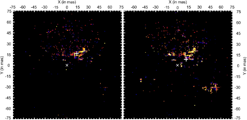
Figure 6: Images of torus model at $0.51$ $\mu$m for two different luminosities and corresponding inner radii, $10^{11}L_{\odot}$ and $R_{in}=0.5$ pc (left panel) and $6\times 10^{11}L_{\odot}$ and $R_{in}=1.16$ pc (right) panel. Photocenter in both panels is denoted with a white cross; black hole in both panels is at the center of the images, denoted with ’x’ The photocenter offset between the images is $8.4$ mas. The values of other torus parameters are the same as in Fig. 5. Images are on a logarithmic scale.

Table 2: The simulated offsets of photocenter (in mas) for different values of redshift and accretion disk luminosity, calculated for the two photometric instruments with central wavelengths at $0.50$ $\mu$m and $0.82$ $\mu$m. The values of torus parameters are the same as in Fig. 5.

$L$	$z$
$(10^{11}L_{\odot})$	0.01	0.05	0.10
$0.50$ $\mu$m
3	1.579	0.208	0.039
6	8.400	1.886	0.860
10	8.170	1.353	0.693
$0.82$ $\mu$m
3	0.814	0.252	0.135
6	7.120	1.422	0.990
10	7.978	1.466	0.843

4.3 Photocenter position vs. flux variation

For one object Taris et al. (2011) found that a relationship between the astrometric and photometric variability exists. We also modeled the expected flux variation with brightness of the perturbed region, and found that the offset of the photocenter in principle can be a function of the flux variation only in special cases where there is a perturbation located at the same place and the brightness changes with time. In general, there are many possible locations of the perturbations and possible values of their emissivities with respect to the central source. The photocenter position varies in terms of both the central source brightness (that may show variability) and the emissivity of the bright spot, hence the relationship between the astrometric and photometric variability cannot be assumed as the general rule, although it may exist particularly in the $\mu$as astrometric regime.

On the other hand, in the case of the changes in the torus structure, as can be seen from Table 2, there is a partial correlation between the photometric and astrometric variability, but it is not a rule, especially when illumination stays higher.

Figure 7: The best fit of the H$\beta$ wavelength band (left), and broad lines (right) after subtracting the narrow components for SDSS J121855.80+020002.1 (up) and SDSS J162011.28+172427 (down). The vertical line corresponds to the position of the narrow component.

5 Observations vs. simulations

The amplitudes of the flux variations in quasars, at certain redshifts, indicate that an enormous amount of energy is produced. The rapid flux variations often seen are convincing evidence of the compactness of the emitting region. Thus, in this case a correlation between astrometric and photometric variability will either not exist or be discerned only with an astrometric precision far higher than the mas level. At the same time, since longer, year-long, and large amplitude variations are also recorded, the same logic would imply that the other quasars elements are not at a standstill, as discussed. The specific causes can be studied when and if an observed long-term, large-amplitude optical variability is related to the astrometric variability of the quasar photocenter (Johnston et al., 2003). In addition, if this were verified, the relationship could indicate that a large photometric variation would make a given quasar less apt to materialize a stable extragalactic reference frame, such as the one from the Gaia mission. The long-term program required to monitor optical fluctuations in long cycles can only be established by ground-based observations. Therefore, the astrometric limit should be on the level of few mas, which, in turn, requires high quality seeing, telescope imaging, and relative astrometry.

We now present observations of the photocenter variability of two objects and discuss the possibility that it was caused by changes to the inner structure of the AGNs.

5.1 Observations

To maximize the chances of the photocenter variability being detected on a mas scale, $20$ quasars were selected based on their long variability timescales and large photo-variability. Most objects were collected from Teerikorpi et al. (2000), as well as Maccacaro et al. (1987) and inspections of light curves in Smith et al. (1993). The observations were performed under the Observatório Nacional/MCT, Brasil, telescope time contracted to ESO at the Max Planck $2.2$ m telescope at La Silla, Chile. The program started on April $2007$ and lasted until July $2009$, with observations taking place about every two months.

The ESO2p2 WFI direct image camera is an array of 2 $\times$ 4 CCDs, each covering a field of $7.5$ $\times$ $15.0$ arcmin, to scale of $0.238$ arcsec/px. For all the observations the same CCD was used, keeping the quasar on a clean spot, at about one third of the diagonal starting from the optical axis. The same configuration was repeated for all the observations of a same quasar, jittering allowed. The observations as a rule were made within two hours of hour angle. Red (Rc/162, peak $651.7$ nm, FWHM $162.2$ nm) and blue (BB#B/123, peak $451.1$ nm, FWHM $135.5$ nm) filters were used for each run. Depending on the quasar magnitude, typically from three to five images were taken with each filter. The integration times were never longer than $30$ min., yet as long as possible to provide good imaging data of the target and the surrounding stars. The combined signa-to-noise ratio was always close to $1000$ for each run.

All images were treated by IRAF MSCRED for trimming, bias substraction, flat-fielding, bad-pixel removal and split. Typically this image processing enhances the SNR by a factor of two. The IRAF DAOFIND and PHOT tasks are employed for the determination of centroid and (instrumental) magnitudes, with the entry parameters adjusted for each frame. Centroids and fluxes are obtained adjusting bi- dimensional Gaussians. The inner ring where the object counting is made and the outer ring where the sky background is counted are variable for each object and frame, but their ratio is kept constant. The plate scale and frame orientation are derived by IRAF IMCOORDS from positions of UCAC2 catalogue stars (though, since the astrometry is totally relative, their values are of no great consequence to define the correlation under study).

Additional aspects of the method described above were presented in Andrei et al. (2009), for the error analysis, and in Andrei et al. (2011), for relative astrometry to derive mas-level variations. A full analysis of the program itself will be presented elsewhere (Andrei et al., 2011). Here we present the preliminary results regarding the R filter, where the WFI sensitivity is higher, for two selected sources (see Table 3), to exemplify the effects discussed in this paper. The relative astrometric and variability procedure initially adjusts the frames one on top of the other, in terms of coordinates and magnitudes, with respect to the quasar position. Next, frame after frame, on the basis of the PHOT data, the objects common to all frames are stored, provided that the (X,Y) coordinates and the magnitudes do not vary above a chosen threshold. The common objects (X,Y) coordinates and magnitudes are then adjusted by a complete third degree polynomial to a mean frame, where C represents either for X, Y or M, given by

$$C_{n}^{m}-<C>_{n}=3DC_{0}+\sum_{i,j,k}^{1,3}A_{i,j,k}^{m}X^{i}Y^{j}M^{k}$$ (7)

Finally, a further round of analysis discards the reference objects for which (X,Y) or magnitude variation are above the threshold. The averages of (X,Y) and magnitude for the remaining objects (with reference to the quasar as a fixed origin) are obtained and correlated with both the time-line and each other.

Table 3 presents the timeline variation in position and magnitude for quasars J121855.80+020002.1 and J162011.28+172427.5, with reference values brought from the CDS. The quantities of final comparison stars were 8 for quasar J121855.80+020002.1, and 30 for quasar J162011.28+172427.5, where we note that for the initial frame-to-frame adjustment the number of stars used was always much larger. As a consequence, the positional errors had a mode of $1.5$ mas for the first object and $15$ mas for the second - whereas the magnitude errors had mode $0.001$ for both objects.

Table 3: . The summary of the measurements of the offset of photocenter: Col. 1 - the mean epoch of observation; Col. 2 - the time interval in days between each measurement; Col. 3 - the X-direction (basically RA) astrometric variation in mas from the previous measurement ; Col. 4 - the Y-direction (basically DEC) astrometric variation in mas from the previous measurement; Col. 5 - the magnitude variation given in tenths of magnitude from the previous measurement. In the first lines, the values correspond to the offsets to the nominal CDS references. In the subsequent lines, we present the offsets to the previous line values. The combined corresponding errors ($\sigma$) are given.

SDSS J121855.80+020002.1, z = 0.327, MAGR = 18m.1
DATE	DAYs	$\Delta$RA$\pm\sigma$	$\Delta$DE$\pm\sigma$	$\Delta$MAG${}_{R}\pm\sigma$
		(mas)	(mas)	(10-1)
2008.016	0.0	-11$\pm$3	- 3$\pm$2	-0.420$\pm$0.009
2008.163	53.4	+15$\pm$3	+ 4$\pm$2	+0.134$\pm$0.007
2008.263	36.8	+ 6$\pm$2	- 3$\pm$1	-0.917$\pm$0.011
2008.415	55.4	- 4$\pm$1	+ 1$\pm$1	+1.774$\pm$0.012
2008.970	202.7	- 8$\pm$1	+ 4$\pm$1	-1.773$\pm$0.007
2009.382	150.5	0$\pm$4	- 3$\pm$2	+2.070$\pm$0.011
SDSS J162011.28+172427.5, z = 0.112, MAGR = 16m.2
DATE	DAYs	$\Delta$RA$\pm\sigma$	$\Delta$DE$\pm\sigma$	$\Delta$MAG${}_{R}\pm\sigma$
		(mas)	(mas)	(10-1)
2007.277	0.0	-17$\pm$10	+24$\pm$22	-0.136$\pm$0.007
2007.430	58.8	+ 2$\pm$9	0$\pm$24	+0.032$\pm$0.007
2008.415	356.9	+14$\pm$6	+ 4$\pm$21	+0.021$\pm$0.006
2008.647	84.9	-23$\pm$8	-59$\pm$16	+0.002$\pm$0.005
2009.181	195.1	+76$\pm$19	+36$\pm$15	+0.550$\pm$0.023
2009.382	73.3	-47 $\pm$18	-58$\pm$22	-0.560$\pm$0.023

From the six values of right ascension and declination variation for the two example sources in Table 3, we can calculate the non-parametric correlations against the magnitude variations. They were calculated by the Spearman rank correlation coefficient, which permitted weighting by the inverse squared sum of the position and magnitude uncertainties. For quasar J121855.80+020002.1, the correlations are $\Delta$RA$\times$$\Delta$MAG=0.44 (significance 0.03) and  $\Delta$DE$\times$$\Delta$MAG=0.56 (significance 0.01). For quasar J162011.28+172427.5, the correlations are $\Delta$RA$\times$$\Delta$MAG=0.75 (significance 0.01)  and  $\Delta$DE$\times$$\Delta$MAG=0.75 (significance 0.01). Consequently, there is no significant correlation between the photocenter and magnitude variation (significance $>>10^{-5}$).

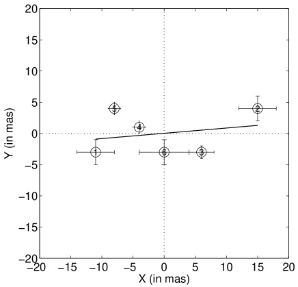
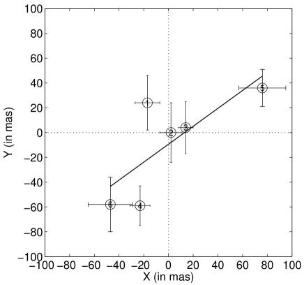
Figure 8: Observed astrometric variability of the photocenter, measured for SDSS J121855.80+020002.1 at $z=0.327$ (up) and SDSS J162011.28+172427.5 (MRK 877) at $z=0.112438$ (down), during the period 2007-2009 (see Table 3). The straight solid lines in the panels represent linear fits through the observed positions. Notations of points from 1 to 5 correspond to the observational epochs from first to the last as given in Table 3.

5.2 Comparison between the simulated and the observed variations

To explore whether the observed variations in SDSS J121855.80+020002.1 ($z=0.327$, $18^{m}.1$) and SDSS J162011.28+172427.5 (Mrk 877, $z=0.112438$, $16^{m}.2$) are caused by perturbations in the accretion disk, we first estimate the masses of the black holes ($M_{bh}$) for these two objects. There are several estimators for $M_{bh}$ in AGN (see e.g McGill et al., 2008, and reference therein), and to measure them for these two objects we used spectra observed with HST (for SDSS J121855.80+020002.1) and from SDSS database (for SDSS J162011.28+172427.5). We first measured from spectra the luminosity at 5100 Å and decomposed spectra using a multi-Gaussian fit (see e.g. Popović et al., 2004). In Fig. 7, the best fit and the broad component after subtraction of the narrow and Fe II lines are shown. As can be seen in Fig. 7, the broad H$\beta$ line in both objects has a red asymmetry, indicating a very complex geometry of the BLR. Also, two separated broad components may indicate the presence of disk emission. After measuring the full width at half maximum (FWHM), we used the three estimators $M_{S}$, $M_{V}$ and $M_{N}$, given by Shields et al. (2003), Vestergaard & Peterson (2006), and Netzer & Trakhtenbrot (2007), respectively. The estimated masses for SDSS J121855.80+020002.1 are: $M_{S}=9.18\times 10^{8}\ M_{\odot}$, $M_{V}=1.37\times 10^{9}\ M_{\odot}$, and $M_{N}=1.10\times 10^{9}\ M_{\odot}$, or on average $M_{bh}=(1.13\pm 0.23)\times 10^{9}\ M_{\odot}$. In the same way, we estimated the black hole masses of SDSS J162011.28+172427.5 to be $M_{S}=3.51\times 10^{8}\ M_{\odot}$, $M_{V}=5.25\times 10^{8}\ M_{\odot}$, $M_{N}=3.72\times 10^{8}\ M_{\odot}$, or on average $M_{bh}=(4.16\pm 0.95)\times 10^{8}\ M_{\odot}$.

To estimate the possibility that the photocenter variability is caused by some perturbation in the disk (or in the BLR), we calculated dimensions of the BLR of these two objects, using the relation between the BLR radius and luminosity at $5100$ Å (see e.g. Vestergaard & Peterson, 2006). We estimated the BLR sizes for SDSS J121855.80+020002.1 to be around $113$ light days (that is $\sim 0.02$ mas) and for Mrk 877 $10$ light days ($\sim 0.004$ mas). Therefore, the observed photocenter variability cannot be explained by the perturbation in the BLR..

5.3 Possible explanation of the photocenter variability in SDSS J121855.80+020002.1 and Mrk 877

As we noted in §5,2, a perturbation in the accretion disk cannot explain the photocenter jitter observed in the two quasars. Moreover, we have estimated that the BLR in both objects is very compact, around 10${}^{-5}-10^{-6}$ arcsec (that translates into light day to several hundred light day scale), which is inconsistent with the photocenter variations. We note that these compact regions cannot be resolved by Gaia, as its PSF will be $\sim 200$ mas.

For objects that are partially obscured, a variation in both the central luminosity and the dust sublimation radius may produce an offset in the photocenter (at z=0.1, see Table 2), of about of one tenth arcsec. However it cannot explain the photocenter of the two quasars under study, as the jitter is smaller, and they both exhibit broad emission lines, which implies that they have a geometry where obscuration is very small or nonexistent.

Another possible source of photocenter variability are “nuclear” super-novae. Several studies (see e.g. Cid Fernandes et al., 2004; Davies et al., 2007; Popović et al., 2009, etc.) demonstrate that AGNs may be associated with star formation regions. For instance Davies et al. (2007) found that on kpc (or pc) scales (corresponding to the observed photocenter variation in our objects) the luminosity of the starburst component may be comparable to that of the AGN.

For the (U)LIRGs (ultra luminous infrared galaxies), the expected supernova rate is very high, as high as $2.4$ yr^-1, if the infrared luminosity is produced entirely by starbursts (Mannucci et al., 2003, see). In the extreme case of this kind of objects, a large supernova rate (SNr) may have influence on the stability of the photocenter. We estimate the SNr, considering the relation given in Mattila & Meikle (2001), and assuming that the SNr and the star formation rate (SFR) are correlated (Mannucci et al., 2003), the latter calculated using the luminosity of the H$\alpha$ line (Calzetti et al., 2007). We could only calculate the SNr for SDSS J121855.80+020002, because we do not have H$\alpha$ spectral data for Mrk 877. We obtained SFR$\approx$14.7 yr^-1 and a corresponding SNr$\approx$0.1 yr^-1 (i.e. one SN every ten years) for SDSS J121855.80+020002. We conclude that it is unlikely that supernovae are responsible for the photocenter shift of this object.

We now discuss a scenario where the photocenter jitter might be related to the jet emission. In terms of radio loudness (Kellermann et al., 1989), i.e. $R=F_{5GHz}/F_{Bband}>10$, SDSS J121855.80+020002.1 has a value of $R\sim 1.1$ (Rafter et al., 2009), and Mrk 877 has $R\sim 0.41$ (Sikora et al., 2007), very far from the values shown by radio loud quasars, which tend to have relativistic jets. Radio-quiet objects can have jet emission (e.g. Mrk 348, see Anton et al., 2002), though their radio-brightness can be significantly higher (Anton et al., 2002) than that of the objects under study. There are VLA $1.4$GHz maps at the position of our sources. The FIRST map of SDSS J121855.80+020002 shows a faint core-morphology on the $1$ mJy level, and in the case of Mrk 877 there is no detection with NVSS at the position of the optical source. We conclude that there is no evidence that the jet plays a role in the photocentric variation of these objects.

It is interesting that in the two objects (see Fig. 8) the photocenter offset is almost aligned, especially in SDSS J121855.80+020002, with a straight line.

These aligned positions of the photocenter offset may correspond to two variable sources close to each other, with the photocenter always shifting towards the brighter of the two. A speculative possibility is a binary supermassive black-hole system, of the type discussed in (see e.g. Lauer & Boroson, 2009; Bogdanović et al., 2009; Shields et al., 2010; Barrows, 2011; Popović, 2011, and references therein), and based on the observations of double-peaked narrow and broad lines. We note that the broad-line shapes of the objects under study are complex (see Fig. 7) and can be properly fitted with two broad Gaussians that are shifted (toward either the blue or red) with respect to the central narrow component (the vertical line in Fig. 7. In Popović et al. (2000) and Shen & Leob (2010), a binary broad emission-line region has been investigated, and the line profiles of this system have been discussed. To detect two peaks in the broad line profile, it is necessary to be able to resolve the two BLRs, and the plane of the orbit must be edge on with respect to the line of observation. An asymmetric line profile might result solely from a system where the two BLRs have different dimensions and luminosities (see Figs. 4-8 in Popović et al., 2000). Such a system might exist at the center of our quasars, and may be the cause of their photocenter variability.

We note that in addition to the binary black hole scenario, the superposition of two visually close and variable sources (see the several examples presented in Popović, 2011) can explain an aligned variability. All of these scenarios should be considered in future investigations.

6 Conclusions

We have simulated the perturbation in the inner structure of quasars (accretion disk and dusty torus), to find how much these effects can offset their photocenters, and try to determine whether it will be observable with future Gaia mission. We have considered two AGNs whose the photocenter variations have been observed, in order to compare them with our simulations. From our investigations, we draw the following conclusions:

i) Perturbations (or bright spots) in an accretion disk may cause an offset of the photocenter, and this effect has a good chance of being detected by the Gaia mission. The most likely candidates are low-redshifted AGNs with massive black holes (10⁹-10¹⁰) that are in principle very bright objects. One can expect a maximal offset of the center (in the case of a bright spot located at disk-edge) on the order of few mas.

ii) A photocenter offset can be caused by changes to the torus structure due to different illuminations of the torus when the central source is obscured by the dust. A maximal offset can be several mas, which also be detectable with Gaia.

iii) A photocenter offset caused by both effects is connected to the photometric variation in the objects, but there is a small probability of a correlation between astrometric and photometric variations. We note here that quasars with high photometric variability are not good objects for constructing the optical reference frame.

iv) To exclude the possibility of the photocenter variation being caused by a perturbation in the accretion disk, or in the BLR, one may estimate the dimensions of the BLR and choose objects with a compact BLR. However, to avoid any variation in the photocenter caused by filaments in the torus, it is preferable to choose quasars with face-on oriented tori.

v) The observed photocenter variability of two quasars cannot be explained by the variation in their inner structure (accretion disk and torus). It seems that the observed photocenter variation can be reproduced very well by a scenario with double variable sources at the center of these objects. It may indicate (as well as complex broad line shapes) that these objects are good candidates for binary black hole systems.

At the end, we conclude that Gaia, in addition to providing astrometrical measurements, may be very useful for an astronomical investigation of the inner quasar structure (physical processes), especially in low redshift variable sources.