Vacuum energy induced by an impenetrable flux tube of finite radius

Abstract

We consider the effect of the magnetic field background in the form of a tube of the finite transverse size on the vacuum of the quantized charged massive scalar field which is subject to the Dirichlet boundary condition at the edge of the tube. The vacuum energy is induced, being periodic in the value of the magnetic flux enclosed in the tube. Our previous study in J. Phys. A: 43, 175401 (2010) is extended to the case of smaller radius of the tube and larger distances from it. The dependence of the vacuum energy density on the distance from the tube and on the coupling to the space-time curvature scalar is comprehensively analyzed.

1 Introduction

The energy which is induced in the vacuum of quantized matter fields that are subject to boundary conditions has been studied intensively over more than six decades since Casimir [1] predicted a force between grounded metal plates, see reviews in Refs. [2] and [3]. The induced vacuum energy in bounded spaces gives rise to a macroscopic force between bounding surfaces. The Casimir force between grounded metal plates has now been measured quite accurately and agrees with his predictions, see, e.g. Refs. [4] and [5], as well as other publications cited in Refs. [2] and [3].

In the present paper we study the vacuum energy which is induced by boundary conditions in space that is not bounded but, instead, is not simply connected, being an exterior to a straight infinitely long tube. This setup is inspired by the famous Aharonov-Bohm effect [6], and we are interested in polarization of the vacuum which is due to imposing a boundary condition at the edge of the tube carrying magnetic flux lines inside itself.

Throughout the present paper, we restrict ourselves to the case of quantized scalar matter. A peculiarity of this case is that the energy-momentum tensor depends on the coupling ($\xi$) of the scalar field to the scalar curvature of space-time even then when space-time is flat. If scalar field is massless, then conformal invariance of the theory is achieved at $\xi=\xi_{c}$, where [7] – [9]

$$\xi_{c}=\frac{d-1}{4d}\,,$$ (1)

and $d$ is the spatial dimension; note that $\xi_{c}$ varies from $0$ to $1/4$ when $d$ varies from $1$ to $\infty$. Up to now the study was restricted to the case of a singular magnetic vortex only [10] – [13], i.e. when the transverse size of the flux-carrying tube is neglected. Therefore, the aim of the present paper is to take account of nonzero transverse size of the flux-carrying tube (for a preliminary study, see Ref. [14]).

2 Vacuum energy density

The operator of the quantized charged scalar field is represented in the form

$$\Psi(x^{0},\vec{x})=\sum\int\limits_{\lambda}\frac{1}{\sqrt{2E_{\lambda}}}\left[e^{-{\rm i}E_{\lambda}x^{0}}\psi_{\lambda}({\bf x})\,a_{\lambda}+e^{{\rm i}E_{\lambda}x^{0}}\psi_{-\lambda}({\bf x})\,b^{\dagger}_{\lambda}\right],$$ (2)

where $a^{\dagger}_{\lambda}$ and $a_{\lambda}$ ($b^{\dagger}_{\lambda}$ and $b_{\lambda}$) are the scalar particle (antiparticle) creation and destruction operators satisfying commutation relations; wave functions $\psi_{\lambda}(\textbf{x})$ form a complete set of solutions to the stationary Klein-Gordon equation

$$\left(-{\mbox{\boldmath$\nabla$}}^{2}+m^{2}\right)\psi_{\lambda}({\bf x})=E^{2}_{\lambda}\psi({\bf x}),$$ (3)

$\nabla$ is the covariant derivative in an external (background) field and $m$ is the mass of the scalar particle; $\lambda$ is the set of parameters (quantum numbers) specifying the state; $E_{\lambda}=E_{-\lambda}>0$ is the energy of the state; symbol $\sum\int\limits_{\lambda}$ denotes summation over discrete and integration (with a certain measure) over continuous values of $\lambda$.

We are considering the static background in the form of the cylindrically symmetric magnetic vortex of finite thickness, hence the covariant derivative is $\mbox{\boldmath$\nabla$}=\mbox{\boldmath$\partial$}-{\rm i}e{\bf V}$ with the vector potential possessing only one nonvanishing component given by

$$V_{\varphi}=\Phi/2\pi$$ (4)

outside the vortex; here $\Phi$ is the vortex flux and $\varphi$ is the angle in the polar $(r,\varphi)$ coordinates on a plane which is transverse to the vortex. The Dirichlet boundary condition on the edge $(r=r_{0})$ of the vortex is imposed on the scalar field:

$$\left.\psi_{\lambda}\right|_{r=r_{0}}=0,$$ (5)

i.e. quantum matter is assumed to be perfectly reflected from the thence impenetrable vortex. Provided the orthonormalization condition is satisfied,

$$\int d^{3}x\psi_{\lambda}^{*}\psi_{\lambda^{\prime}}=\langle\lambda|\lambda^{\prime}\rangle,$$ (6)

the solution to (3) and (5) in the case of the impenetrable magnetic vortex of thickness $2r_{0}$ takes form

$$\psi_{knk_{z}\,}({\bf x})=(2\pi)^{-1}e^{{\rm i}k_{z}z}e^{{\rm i}n\varphi}\beta_{n}(kr_{0})\times\\ \times[Y_{|n-e\Phi/2\pi|}(kr_{0})J_{|n-e\Phi/2\pi|}(kr)-J_{|n-e\Phi/2\pi|}(kr_{0})Y_{|n-e\Phi/2\pi|}(kr)],$$ (7)

where $z$ is the coordinate along the vortex,

$$\beta_{n}(kr_{0})=\left[Y^{2}_{|n-e\Phi/2\pi|}(kr_{0})+J^{2}_{|n-e\Phi/2\pi|}(kr_{0})\right]^{-1/2}\!\!,$$ (8)

and $0<k<\infty$, $-\infty<k_{z}<\infty$, $n\in\mathbb{Z}$ ($\mathbb{Z}$ is the set of integer numbers); $J_{\mu}(u)$ and $Y_{\mu}(u)$ are the Bessel functions of order $\mu$ of the first and second kinds.

In general, the vacuum energy density is determined as the vacuum expectation value of the time-time component of the energy-momentum tensor, that is given formally by expression

$$\varepsilon=\langle\rm vac|\left[\partial_{0}\Psi^{\dagger}\partial_{0}\Psi+\partial_{0}\Psi\partial_{0}\Psi^{\dagger}-(\xi-1/4)\mbox{\boldmath$\nabla$}^{2}(\Psi^{\dagger}\Psi+\Psi\Psi^{\dagger})\right]|\rm vac\rangle=\\ =\sum\int\limits_{\lambda}E_{\lambda}\psi^{*}_{\lambda}(\textbf{x})\,\psi_{\lambda}(\textbf{x})-(\xi-1/4)\mbox{\boldmath$\nabla$}^{2}\sum\int\limits_{\lambda}E^{-1}_{\lambda}\psi^{*}_{\lambda}(\textbf{x})\,\psi_{\lambda}(\textbf{x}).$$ (9)

In the following we shall restrict our consideration to the plane $z=0$ which is orthogonal to the vortex.

Thus, the renormalized vacuum energy density in the case of the finite-thickness vortex takes form

$$\varepsilon_{ren}=\frac{1}{2\pi}\left\{\int\limits_{0}^{\infty}dk\,k\left(k^{2}+m^{2}\right)^{1/2}\left[S(kr,kr_{0})-S(kr,kr_{0})|_{\Phi=0}\right]-\right.\\ \left.-(\xi-1/4)\triangle\int\limits_{0}^{\infty}dk\,k\left(k^{2}+m^{2}\right)^{-1/2}\left[S(kr,kr_{0})-S(kr,kr_{0})|_{\Phi=0}\right]\right\},$$ (10)

where, in view of (7),

$$S(kr,kr_{0})=\sum_{n\in\mathbb{Z}}\beta_{n}^{2}(kr_{0})\times\\ \times\left[Y_{|n-e\Phi/2\pi|}(kr_{0})J_{|n-e\Phi/2\pi|}(kr)-J_{|n-e\Phi/2\pi|}(kr_{0})Y_{|n-e\Phi/2\pi|}(kr)\right]^{2},$$ (11)

and $\triangle=\partial^{2}_{r}+r^{-1}\partial_{r}\,$ is the transverse radial part of the laplacian.

Owing to the infinite range of summation, the last expression is periodic in flux $\Phi$ with a period equal to $2\pi e^{-1}$, i.e. it depends on quantity

$$F=\frac{e\Phi}{2\pi}-\left[\!\left[\frac{e\Phi}{2\pi}\right]\!\right],$$ (12)

where $[[u]]$ is the integer part of quantity $u$ (i.e. the integer which is less than or equal to $u$).

Let us rewrite (11) in the form

$$S(kr,kr_{0})=S_{0}(kr)+S_{1}(kr,kr_{0}),$$ (13)

where $S_{0}(kr)$ corresponds to the appropriate series in the case of the vacuum polarization by a singular magnetic vortex [11] – [13]:

$$S_{0}(kr)=\sum_{n=0}^{\infty}\left[J^{2}_{n+F}(kr)+J^{2}_{n+1-F}(kr)\right]=\int\limits_{0}^{kr}\!d\tau\left[J_{F}(\tau)J_{-1+F}(\tau)+J_{-F}(\tau)J_{1-F}(\tau)\right],$$ (14)

and $S_{1}(kr,kr_{0})$ is a correction term due to the finite thickness of a vortex:

$$S_{1}(kr,kr_{0})=2\sum_{n=0}^{\infty}\left[J_{n+F}(kr_{0})Y_{n+F}(kr)\frac{J_{n+F}(kr_{0})Y_{n+F}(kr)-Y_{n+F}(kr_{0})J_{n+F}(kr)}{J_{n+F}^{2}(kr_{0})+Y_{n+F}^{2}(kr_{0})}\right.+\\ +\left.J_{n+1-F}(kr_{0})Y_{n+1-F}(kr)\frac{J_{n+1-F}(kr_{0})Y_{n+1-F}(kr)-Y_{n+1-F}(kr_{0})J_{n+1-F}(kr)}{J_{n+1-F}^{2}(kr_{0})+Y_{n+1-F}^{2}(kr_{0})}\right]-\\ -\sum_{n=0}^{\infty}\left[J_{n+F}^{2}(kr_{0})\frac{J_{n+F}^{2}(kr)+Y_{n+F}^{2}(kr)}{J_{n+F}^{2}(kr_{0})+Y_{n+F}^{2}(kr_{0})}+J_{n+1-F}^{2}(kr_{0})\frac{J_{n+1-F}^{2}(kr)+Y_{n+1-F}^{2}(kr)}{J_{n+1-F}^{2}(kr_{0})+Y_{n+1-F}^{2}(kr_{0})}\right].$$ (15)

In the absence of the magnetic flux in the tube we have

$$S(kr,kr_{0})|_{\Phi=0}=\tilde{S}_{0}+\tilde{S}_{1}(kr,kr_{0}),$$ (16)

where

$$\tilde{S}_{0}=J^{2}_{0}(kr)+2\sum_{n=1}^{\infty}J^{2}_{n}(kr)=1,$$ (17)

and a correction term due to the finite thickness of an empty tube:

$$\tilde{S}_{1}(kr,kr_{0})=2\left[J_{0}(kr_{0})Y_{0}(kr)\frac{J_{0}(kr_{0})Y_{0}(kr)-Y_{0}(kr_{0})J_{0}(kr)}{J_{0}^{2}(kr_{0})+Y_{0}^{2}(kr_{0})}\right.+\\ +\left.2\sum_{n=1}^{\infty}J_{n}(kr_{0})Y_{n}(kr)\frac{J_{n}(kr_{0})Y_{n}(kr)-Y_{n}(kr_{0})J_{n}(kr)}{J_{n}^{2}(kr_{0})+Y_{n}^{2}(kr_{0})}\right]-\\ -\left[J_{0}^{2}(kr_{0})\frac{J_{0}^{2}(kr)+Y_{0}^{2}(kr)}{J_{0}^{2}(kr_{0})+Y_{0}^{2}(kr_{0})}+2\sum_{n=1}^{\infty}J_{n}^{2}(kr_{0})\frac{J_{n}^{2}(kr)+Y_{n}^{2}(kr)}{J_{n}^{2}(kr_{0})+Y_{n}^{2}(kr_{0})}\right].$$ (18)

Thus, vacuum energy density (10) depends on $F$ (12), i.e. it is periodic in flux $\Phi$ with a period equal to $2\pi e^{-1}$. Moreover, relation (10) is symmetric under substitution $F\rightarrow 1-F$, vanishing at $F\rightarrow 0$ $(F\rightarrow 1)$ and, perhaps, attaining its maximal value at $F=1/2$. Relations (14) and (15) are simplified at $F=1/2$:

$$S_{0}(kr)|_{\Phi=\pi e^{-1}}=\frac{2}{\pi}\int\limits_{0}^{2kr}\frac{d\,\tau}{\tau}\sin\tau,$$ (19)

and

$$S_{1}(kr,kr_{0})|_{\Phi=\pi e^{-1}}=\\ =\!2\!\sum_{n=0}^{\infty}\frac{J_{n+\frac{1}{2}}^{2}(kr_{0})\!\left[Y_{n+\frac{1}{2}}^{2}(kr)\!-\!J_{n+\frac{1}{2}}^{2}(kr)\right]\!-\!2J_{n+\frac{1}{2}}(kr_{0})Y_{n+\frac{1}{2}}(kr_{0})J_{n+\frac{1}{2}}(kr)Y_{n+\frac{1}{2}}(kr)}{J_{n+\frac{1}{2}}^{2}(kr_{0})+Y_{n+\frac{1}{2}}^{2}(kr_{0})}.$$ (20)

Since it is hardly possible to evaluate sums in (15) and (18) analytically, our further analysis will employ numerical calculation. In the following we restrict ourselves to the case of $F=1/2$, when the expression for the vacuum energy density takes form

$$\varepsilon_{ren}=\frac{1}{2\pi}\left\{\int\limits_{0}^{\infty}dk\,k\left(k^{2}+m^{2}\right)^{1/2}G(kr,kr_{0})-\right.\\ \left.-(\xi-1/4)\triangle\int\limits_{0}^{\infty}dk\,k\left(k^{2}+m^{2}\right)^{-1/2}G(kr,kr_{0})\right\},$$ (21)

where

$$G(kr,kr_{0})=S(kr,kr_{0})|_{\Phi=\pi e^{-1}}-S(kr,kr_{0})|_{\Phi=0}.$$ (22)

3 Numerical evaluation of the vacuum energy density

Following Ref. [14] we rewrite (21) in the dimensionless form

$$r^{3}\varepsilon_{ren}=\alpha_{+}(mr_{0},mr)-(\xi-1/4)r^{3}\triangle\frac{\alpha_{-}(mr_{0},mr)}{r},$$ (23)

where

$$\alpha_{\pm}(mr_{0},mr)=\frac{1}{2\pi}\int\limits_{0}^{\infty}dz\,z\left[z^{2}+\left(\frac{mr_{0}}{\lambda}\right)^{2}\right]^{\pm 1/2}G(z,\lambda z),$$ (24)

and $\lambda=r_{0}/r$, $\lambda\in[0,1]$. Let us point out some analytical properties of the integrand function in (23): it vanishes at the edge of the vortex

$$\lim_{\lambda\rightarrow 1}G(z,\lambda z)=0;$$ (25)

at large distances from the vortex the case of a singular vortex is recovered

$$\lim_{\lambda\rightarrow 0}G(z,\lambda z)=S_{0}(z)|_{\Phi=\pi e^{-1}}-\tilde{S}_{0};$$ (26)

at small values of $z$ one gets

$$G(z,\lambda z)|_{z\rightarrow 0}=-[\ln(\lambda)/\ln(\lambda z)]^{2}.$$ (27)

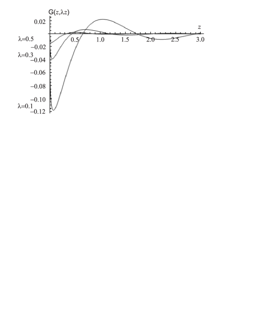
Figure 1: Behavior of $G(z,\lambda z)$ at different values of $\lambda$.

Numerical analysis indicates that in the calculation of function $G(z,\lambda z)$ one can use series in (18) and (20) with finite limits, namely for calculation $G(z,\lambda z)$ at point $z=z^{\prime}$ it is enough to cut off the summation limits by some value $n$ that can be found from condition

$$\left|\frac{G(z,\lambda z)|_{n}-G(z,\lambda z)|_{N}}{G(z,\lambda z)}\right|<\delta(\lambda),\quad\delta(\lambda)<10^{-17},$$ (28)

where $N$ is a big number $N\sim 10^{2}$, $n<N$. It can be shown that the envelope of $G(z,\lambda z)$ is exponentially decreasing function at large $z$, see Fig.1. So, for the finite-thickness magnetic vortex we can compute values of dimensionless quantity $r^{3}\varepsilon_{ren}$ (23) for different values of $\lambda$. To do this, we have to be able to perform integration in (23) with high precision. We make it in a following way.

As one can see from Fig.2, the function $G(z,\lambda z)$ is negative from $z=0$ to the first function root at $z=z_{1}$ ($z_{1}\neq 0$). So, the appropriate integral in (21) is negative. The subsequent roots are denoted by $z_{2}$, $z_{3}$, etc. Because of decreasing character of the envelope function the integral from $z_{1}$ to $z_{3}$ will be positive. It is useful to define a period of function $G(z,\lambda z)$ as an interval between two next to neighboring roots, i.e. from $z_{1}$ to $z_{3}$, from $z_{3}$ to $z_{5}$, and so on. Then the full integral in (21) will be a sum of the negative integral from $z=0$ to $z=z_{1}$ and a multitude of positive integrals over subsequent periods. In the case of sufficiently small transverse size of the tube ($mr_{0}\ll 1$) the integrals over some finite number of first periods may be negative but thereupon they become and remain positive also.

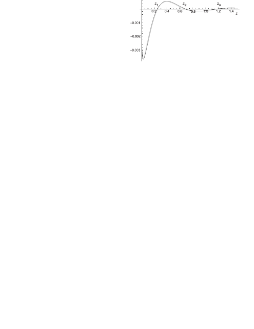
Figure 2: The location of roots of $G(z,\lambda z)$ at $\lambda=0.7$.

For small $z$ we make a direct integration of function $G(z,\lambda z)$ over periods. For large $z$ we make integration for each period separately. To do it we create a table of values of function $G(z,\lambda z)$ for a separate period and replace this function by a more simple function in the form

$$G_{int}(z,\lambda z)=a\frac{e^{-bz}}{z^{c}}\frac{A_{q}(z^{2})}{B_{q}(z^{2})}\sin(kz+j\ln z+\phi_{0}),$$ (29)

where sine function ensures that roots of $G_{int}(z,\lambda z)$ coincide with roots of $G(z,\lambda z)$; $A_{q}(y)$ and $B_{q}(y)$ are $q$-degree polynomials, $q$ can be 3, 4 or 5; all unknown parameters can be found from an interpolation procedure. We allow a relative error of interpolation to be

$$\left|\frac{G_{int}(z,\lambda z)-G(z,\lambda z)}{G(z,\lambda z)}\right|<10^{-8}$$ (30)

for each period. The function $G_{int}(z,\lambda z)$ can be immediately integrated with the required accuracy.

With the help of the above procedure we obtain a table of contributions from integration over each period, extrapolate this table to infinity, and after that we find the full integral in (21) as a sum of the negative integral over first period(s), a multitude of positive integrals over periods and an interpolation term.

For $\alpha_{+}$ function we estimate the relative error of the obtained result as $0.1\%$. It should be noted that nearly 95 % of the integral value is obtained by direct calculation and only nearly 5% is the contribution from the interpolation. The integration in $\alpha_{-}$ function is performed more quickly and with a higher accuracy, as compared to the case of $\alpha_{+}$ function, because of its more rapid decreasing at large distances. In this case the contribution from the interpolation can be $10^{-3}\%$ from the final value of integration.

Dimensionless quantity $r^{3}\varepsilon_{ren}$ (23) can be interpreted as a function of two dimensionless parameters, $mr_{0}$ and $mr$. Using the above described procedure, we calculate $\alpha_{+}$ and $\alpha_{-}$ functions at fixed values of $mr_{0}$ ($mr_{0}=1;\,10^{-1};\,10^{-2}$) at some set of points of dimensionless distance from the center of the vortex. This allows us to obtain coefficients of the interpolation function that is found in the form

$$\alpha_{\pm}(x_{0},x)=\left[\pm e^{-2x}x^{1\mp 1/2}\right]\left[\left(\frac{x-x_{0}}{x}\right)^{2}\frac{P^{\pm}_{3}(x-x_{0})}{x^{3}}\right]\frac{Q^{\pm}_{3}(x^{2})}{x^{6}},\quad x>x_{0},$$ (31)

where $x=mr$, $x_{0}=mr_{0}$ and $P^{\pm}_{n},Q^{\pm}_{n}$ — are polynomials of n-th order. First factor in the square bracket in (31) describes the large distance behavior of the appropriate functions in the case of the singular vortex [13], second factor in the square bracket is an asymptotic at small distances from the edge of the tube, and the last factor is the intermediate part of the function. Since the flux tube is impenetrable, the $\alpha_{\pm}$ functions are zero at $x\leq x_{0}$. Behavior of the dimensionless $\alpha_{\pm}$ functions is presented on Fig.3.

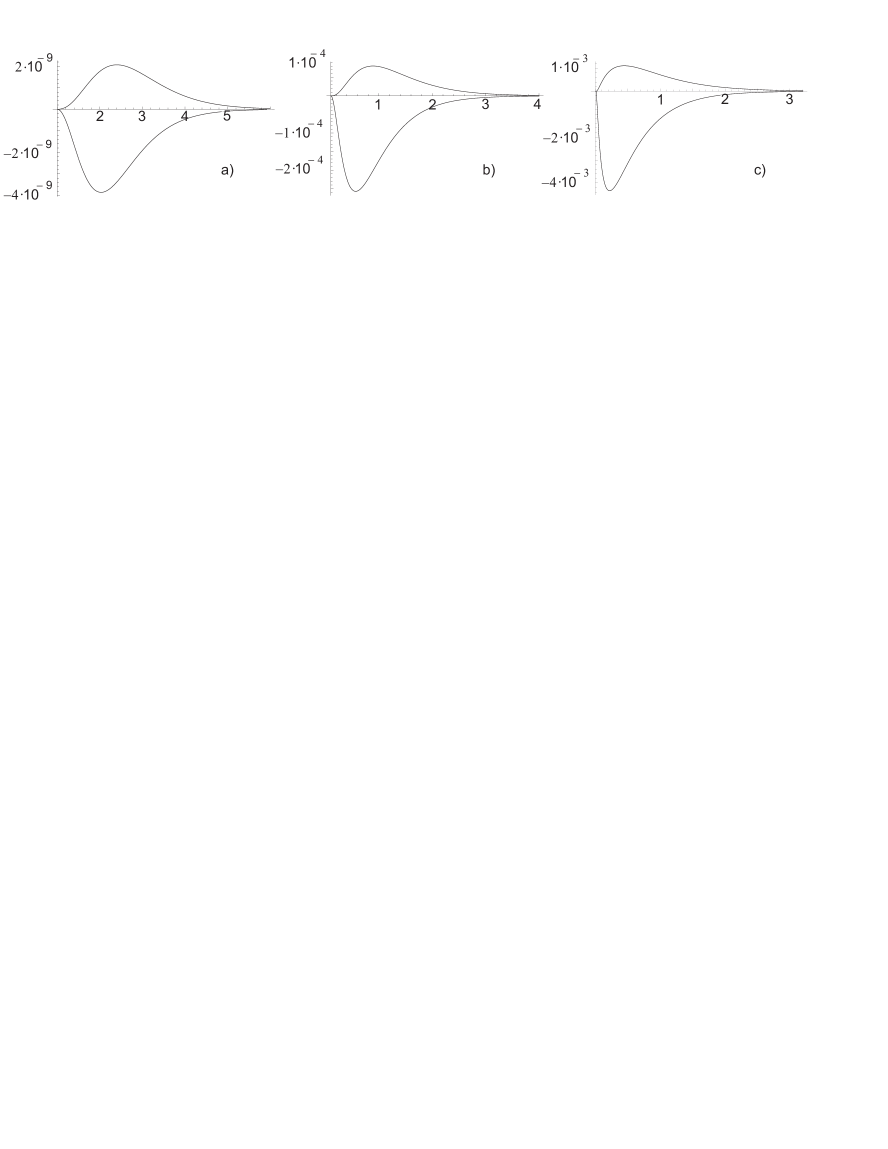
Figure 3: Behavior of the $\alpha_{+}(x_{0},x)$ (positive) and the $\alpha_{-}(x_{0},x)$ (negative) functions for the case of a) $x_{0}=1$, b) $x_{0}=10^{-1}$, c) $x_{0}=10^{-2}$. The variable $x$ $(x>x_{0})$ is along the abscissa axis.

We define function

$$\tilde{\alpha}_{-}(x_{0},x)=r^{3}\triangle\left(\frac{\alpha_{-}(x_{0},x)}{r}\right)=\alpha_{-}(x_{0},x)-x\frac{\partial\alpha_{-}(x_{0},x)}{\partial x}+x^{2}\frac{\partial^{2}\alpha_{-}(x_{0},x)}{\partial x^{2}}.$$ (32)

and present its behavior on Fig.4.

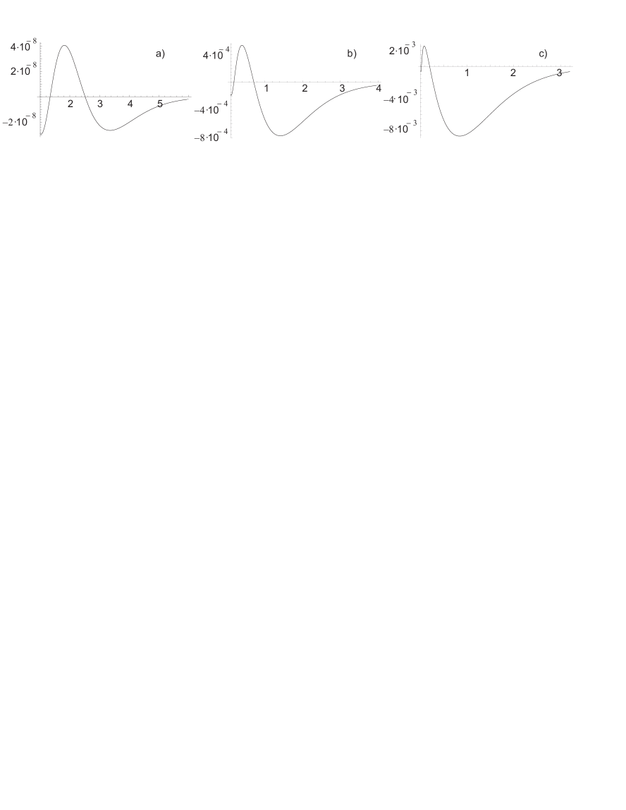
Figure 4: Behavior of the $\tilde{\alpha}_{-}(x_{0},x)$ function for the case of a) $x_{0}=1$, b) $x_{0}=10^{-1}$, c) $x_{0}=10^{-2}$. The variable $x$ $(x>x_{0})$ is along the abscissa axis.

Now we can construct the dimensionless vacuum energy density at different values of the coupling to the space-time curvature scalar:

$$r^{3}\varepsilon_{ren}=\alpha_{+}(x_{0},x)-(\xi-1/4)\tilde{\alpha}_{-}(x_{0},x).$$ (33)

Its behavior is presented on Fig.5 and Fig.6. The case of the singular magnetic vortex [13] is presented on Fig.7.

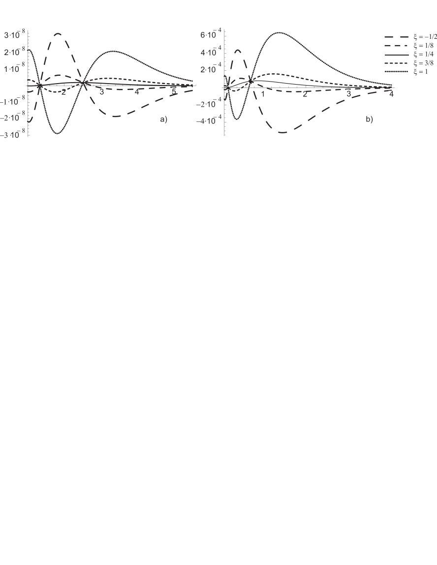
Figure 5: The dimensionless vacuum energy density $r^{3}\varepsilon_{ren}(x_{0},x)$ at different values of the coupling to the space-time curvature scalar for the case of a) $x_{0}=1$, b) $x_{0}=10^{-1}$. The variable $x$ $(x>x_{0})$ is along the abscissa axis.

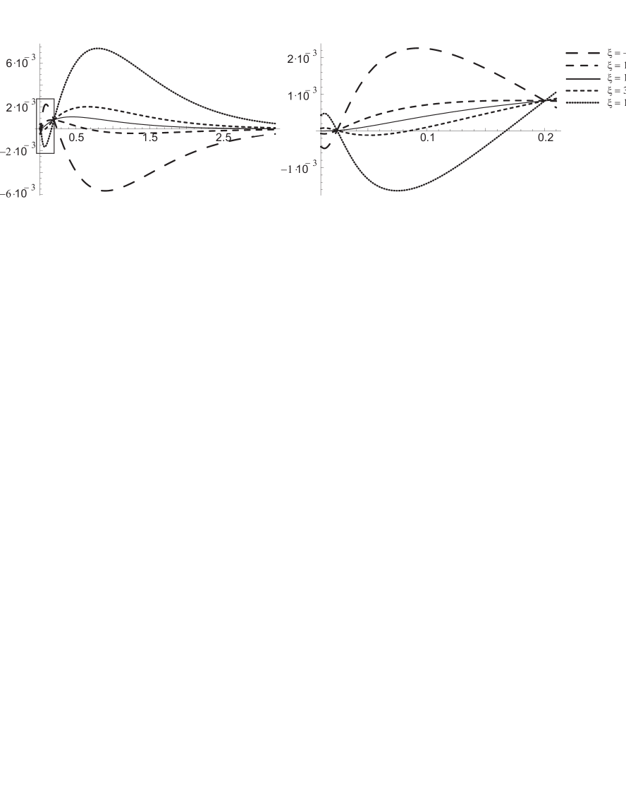
Figure 6: The dimensionless vacuum energy density $r^{3}\varepsilon_{ren}(x_{0},x)$ at different values of the coupling to the space-time curvature scalar for the case of $x_{0}=10^{-2}$. The region in a rectangle on the left figure is seen in the scaled-up form on the right figure. The variable $x$ $(x>x_{0})$ is along the abscissa axis.

The analytical form of the vacuum energy density allows us to obtain the total induced vacuum energy

$$E=\int\limits_{0}^{2\pi}d\varphi\int\limits_{r_{0}}^{\infty}\varepsilon_{ren}\,rdr=2\pi m\left[\int\limits_{x_{0}}^{\infty}\frac{\alpha_{+}(x_{0},x)}{x^{2}}\,dx-(\xi-1/4)\int\limits_{x_{0}}^{\infty}\frac{\tilde{\alpha}_{-}(x_{0},x)}{x^{2}}\,dx\right]\!.$$ (34)

The integral over the $\tilde{\alpha}_{-}$ function (32) can be taken by parts, yielding

$$\int\limits_{x_{0}}^{\infty}\frac{\tilde{\alpha}_{-}(x_{0},x)}{x^{2}}\,dx=-\left.\frac{\partial\alpha_{-}(x_{0},x)}{\partial x}\right|_{x=x_{0}}$$ (35)

In this respect the question about the small distance behavior of the $\alpha_{-}$ function is very important. We have made a numerical calculations at small distances from the tube ($x-x_{0}\sim 10^{-6}x_{0}$) and confirm the quadratic behavior near the edge of the tube (31) $\lim\limits_{x\rightarrow x_{0}}\alpha_{-}(x_{0},x)\sim(x-x_{0})^{2}$. So, quantity (35) is zero, and the $\tilde{\alpha}_{-}$ function affects only the local properties of the vacuum energy density. The total vacuum energy is defined exclusively by the $\alpha_{+}$ function and is independent of $\xi$:

$$E=2\pi m\int\limits_{x_{0}}^{\infty}\frac{\alpha_{+}(x_{0},x)}{x^{2}}\,dx.$$ (36)

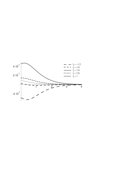
Figure 7: The dimensionless vacuum energy density $r^{3}\varepsilon_{ren}(x_{0},x)$ at different values of the coupling to the space-time curvature scalar for the case of the singular magnetic vortex.

The total vacuum energy (in $2\pi m$ units) of the impenetrable flux tube is $6.94\cdot 10^{-10}$, $1.65\cdot 10^{-4}$, and $1.06\cdot 10^{-2}$ for the case of $x_{0}=1$, $x_{0}=10^{-1}$, $x_{0}=10^{-2}$ correspondingly. It should be noted that the total energy is infinite [13] in the case of a singular magnetic vortex.

The induced vacuum energy density in the units of $m^{3}$ is presented on Fig.8. The results for the case of $\xi=1/4$ are vanishingly small as compared to cases of other values of $\xi$, so they are not visible on Fig.8.

4 Discussion

In the present paper we have considered the energy density which is induced in the vacuum outside a magnetic flux enclosed into an impenetrable tube of finite radius $r_{0}$. Whereas the induced vacuum energy density is divergent at small distances as $r^{-3}$ when the radius is neglected ($r_{0}=0$), see Fig.7, it becomes finite when the radius is taken into account. A very characteristic feature is the appearance of oscillations in the vicinity of the tube, see Fig.5 and Fig.6. Another peculiarity is that curves corresponding to different values of $\xi$ are symmetric with respect to the curve corresponding to $\xi=1/4$, the latter yielding the minimal absolute values of the vacuum energy density, see also Fig.8. The maximal values of the vacuum energy density are becoming hardly observable for $mr_{0}>1$, however, they are quite conspicuous for $mr_{0}<10^{-2}$. This result was obtained earlier [14], but a completely new result concerns the behavior at large distances from the tube (up to $200\,r_{0}$), as well as at different values of $\xi$. It should be noted that the vacuum energy density in the vicinity of the tube is negative at $\xi<1/4$, including the important cases of conformal coupling $\xi=1/8$ (see (1) at $d=2$) and minimal coupling $\xi=0$.

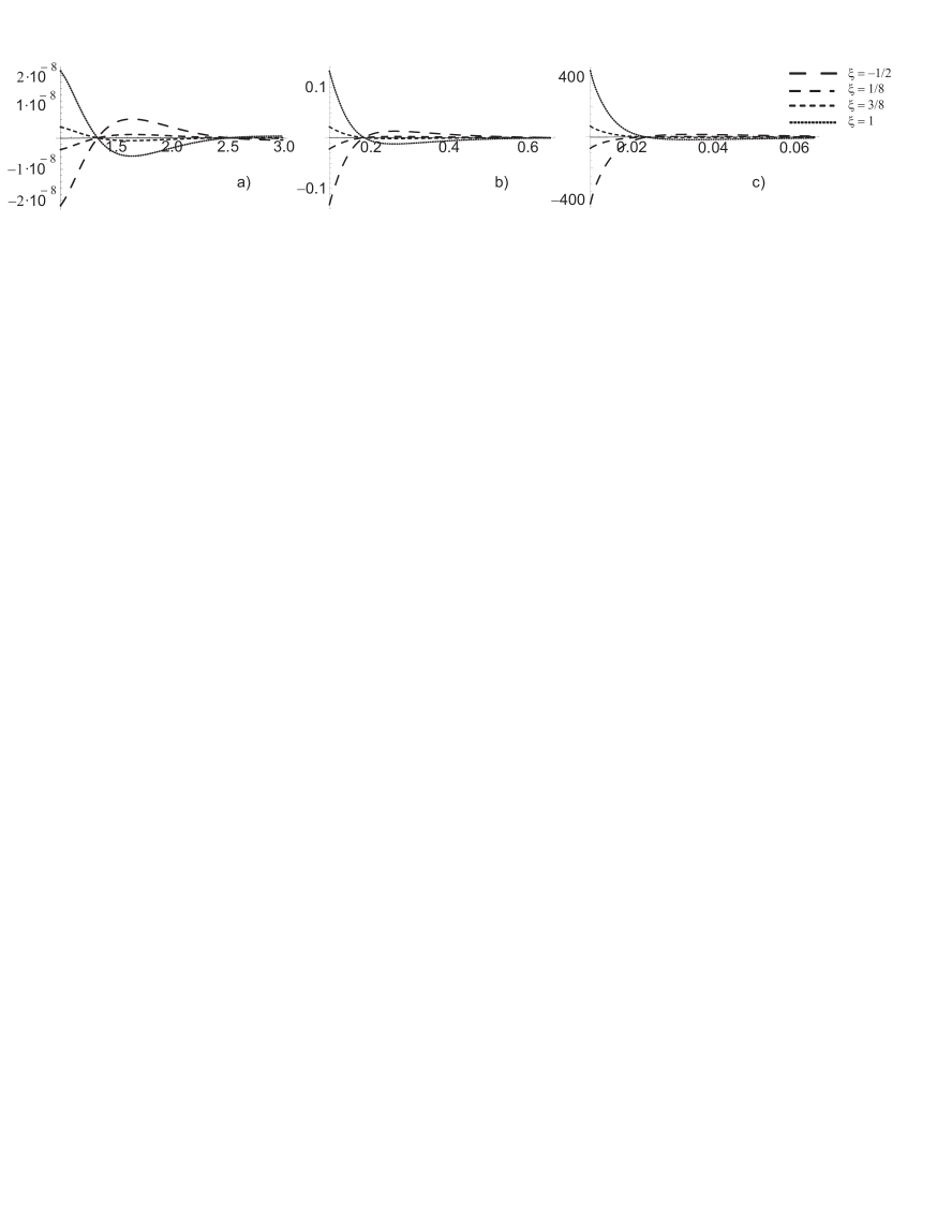
Figure 8: The vacuum energy density $\varepsilon_{ren}(x_{0},x)$ (in $m^{3}$ units) at different values of the coupling to the space-time curvature scalar for the case of a) $x_{0}=1$, b) $x_{0}=10^{-1}$, c) $x_{0}=10^{-2}$.

Since the vacuum energy density is finite, the total vacuum energy, see (34), is finite as well. We show that the latter is positive and independent of $\xi$. Being negligible in the case of $mr_{0}\gtrsim 1$, it produces an appreciable effect of order of $10^{-2}m$ in the case of $mr_{0}=10^{-2}$.